
Flow Field Explorations in a Boundary Layer Pump Rotor for Improving 1D Design Codes
by
 , , , , and
Rosa Freschi
1,
Agapi Bakogianni
1,
David John Rajendran
1,*,
Eduardo Anselmi Palma
1,
Lorenzo Talluri
2 and
Ioannis Roumeliotis
1 1
Centre for Propulsion and Thermal Power Engineering, Cranfield University, Bedford MK43 0AL, UK
2
Department of Industrial Engineering, University of Florence, 50121 Firenze, Italy
*
Author to whom correspondence should be addressed.
Designs 2023, 7(1), 29; https://doi.org/10.3390/designs7010029
Submission received: 1 December 2022
/
Revised: 23 January 2023
/
Accepted: 28 January 2023
/
Published: 3 February 2023
(This article belongs to the Section Mechanical Engineering Design)
Abstract
:Boundary layer pumps, although attractive due to their compactness, robustness and multi-fluid and phase-handling capability, have been reported to have low experimental efficiencies despite optimistic predictions from analytical models. A lower-order flow-physics-based analytical model that can be used as a 1D design code for sizing and predicting pump performance is described. The rotor component is modelled by means of the Navier–Stokes equations as simplified using velocity profiles in the inter-disk gap, while the volute is modelled using kinetic-energy-based coefficients inspired by centrifugal pumps. The code can predict the rotor outlet and overall pump pressure ratio with an around 3% and 10% average error, respectively, compared to the reference experimental data for a water pump. Moreover, 3D RANS flow-field explorations of the rotor are carried out for different inter-disk gaps to provide insights concerning the improvement of the 1D design code for the better prediction of the overall pump performance. Improvements in volute loss modelling through the inclusion of realistic flow properties at the rotor outlet rather than the detailed resolution of the velocity profiles within the rotor are suggested as guidelines for improved predictions. Such improved design codes could close the gap between predictions and experimental values, thereby paving the way for the appropriate sizing of boundary layer pumps for several applications, including aircraft thermal management.
1. Introduction
Thermal management systems are considered an essential technology for enabling zero-carbon emission commercial flights. Research projects such as FlyZero [1] have established technological roadmaps, identifying areas of research where more effort should be applied to achieve the use of green liquid hydrogen in fuel cells, gas turbines and hybrid systems in aircrafts. In the three applications mentioned, thermal management is an area of research that will play a fundamental role. Typically, thermal management challenges are associated with the design of lighter heat exchangers. In addition to that for addressing heat rejection cycles (in the form of vapour compression or liquid closed loops), the design of new compressors and pumps would be required. Boundary layer pumps [2] appear to be strong candidates, given their potential robustness and simplicity of both design and manufacture. Their known capability in terms of handling liquid/solid/gas mixtures [3] and fluids with variant viscosity [4], including blood [5,6], as well as the expected favourable cavitation characteristics [7], further support their suitability for thermal management applications. A boundary layer pump capable of handling fluids, such as the refrigerants R1233zd(E) and R1234yf and carbon dioxide, has been proposed by the authors [8], with the results showing that the theoretical pump’s efficiencies above 50% can be achieved for low mass flow rates and relatively high-pressure ratios.
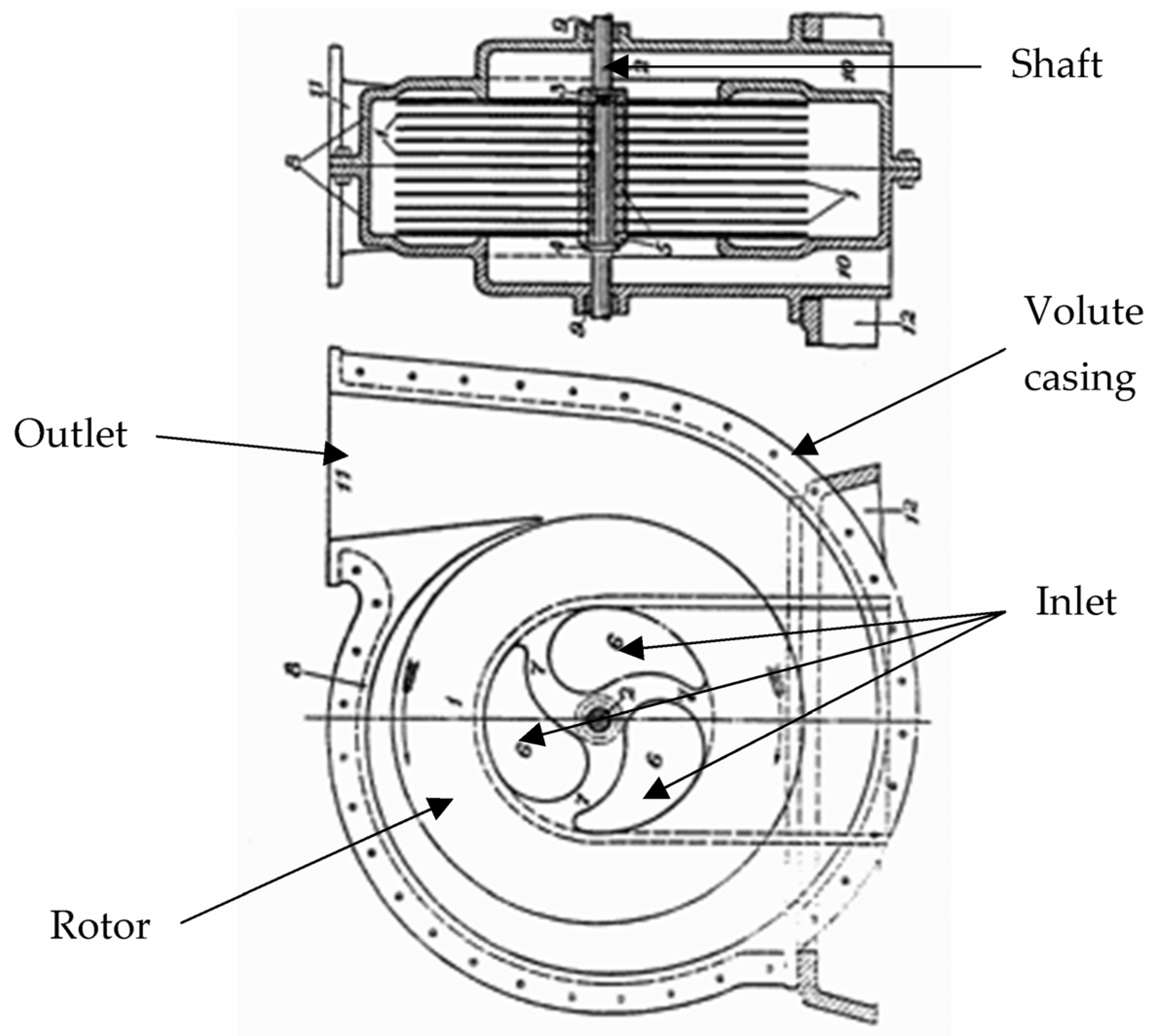
The bladeless impeller device is a rotary pump composed of multiple equally spaced coaxial parallel plane disks mounted on a rotating shaft. The fluid enters through the axial ports at the centre of the discs and is then propelled inside the gaps formed by the axial clearance between the disks. The energy is imparted as the shear stress acting on the fluid by the rotating disks. The spinning also induces a field of centrifugal stresses acting on the flow. The combination of the tangential force due to the rotation and the radial force due to the centrifugal effect leads to a spiral flow path from the inner to the outer diameter of a disk. The rotor pack is enveloped by a volute casing, which collects the flow from the gaps and conveys it towards the outlet of the pump, as shown in Figure 1 [2].
A review reveals that the literature on boundary layer turbomachinery can be broadly classified into four groups. First, studies that deal with the use of analytical and numerical modelling along with experimental campaigns in a few cases for design development and optimisation. Second, studies that propose design modifications for improving the performance of the turbomachine. In this group are also parametric studies that explore the effects of design variables on the turbomachine behaviour. Third, studies that shed light on the loss mechanisms with the objective of explaining the oft-reported low efficiencies of these turbomachines. Fourth, studies that demonstrate the design and application of the boundary layer turbomachinery for special applications. In addition to this classification, each group of which is briefly explained below, a common observation regarding the boundary layer turbomachinery literature is that most of the studies deal with turbines, whereas only a few are about pumps.
In terms of the studies that deal with the design development of boundary layer turbomachines, Guha and Sengupta [9] developed and formulated non-dimensional numbers that can be used for the design and dynamic scaling of Tesla turbines. Song et al. [10] developed a one-dimensional model using the nozzle limit expansion ratio and rotor radial pressure gradients to analyse the performance of a Tesla turbine and noted good agreement with the experimental data. An analytical model based on a simplified, incompressible Navier–Stokes equation for predicting the flow in turbine rotors alone was proposed by Schosser et al. [11]. This model was used for the accuracy assessment of the simplified performance prediction method. Furthermore, an efficiency-based optimisation study in a Tesla turbine was conducted by Rusin et al., who noted the improvement of efficiency from 9% to 17% [12]. A topology optimisation based on a two-dimensional swirl flow model was developed for Tesla pumps by Alonso et al. using an interior point optimisation algorithm based on a finite element solver [13]. This method was used to provide general guidelines on the parametric effects of different design parameters on the pump performance at different regimes. It is observed from these design development and optimisation studies that while the integrated high-fidelity optimisation of the turbomachines has been attempted and described, a simple 1D design code for boundary layer pumps that can be used for the preliminary sizing of specified requirements has not yet been formulated from fluid dynamic principles.
Several design modification studies have been described in the literature, along with detailed parametric effect explorations of the design variables that shed light on the influence of these designs on performance. Galindo et al. [14] studied the effect of disc spacing and pressure flow on a Tesla turbine using both experimental and numerical analysis. Renuke et al. [15] conducted an extensive numerical and experimental investigation of small-scale Tesla turbines and documented the effects of several design parameters, such as the disk thickness, gaps, radius ratios, and outlet areas, in addition to the operating regime, on the machine performance. Romanin et al. [16] proposed strategies for the performance enhancement of Tesla turbines from an operation perspective for combined heat and power applications. Dodsworth and Groulx [17] conducted an operational parametric study involving disk pack spacing and rotational speed for Tesla pumps by considering both performance and structural integrity [18]. Martinez-Diaz et al. conducted a design exploration to understand the effect of turbulisation on the disc pump performance [19]. These design and parametric studies indicate that a reasonable understanding of the effects of design parameters on performance is available in the literature, although a simple 1D code that can tie together the parametric designs to produce workable designs is not yet reported.
An interesting consideration in these recent studies and in the historical literature is the reasonably consistent observation that the efficiency of boundary layer turbomachines is significantly lower than that of conventional bladed turbomachines and the apparent disconnect between the expected efficiencies from numerical studies and the measured experimental efficiencies. To explain the reason for the low efficiencies, detailed computational studies to identify the loss mechanisms were conducted by Wang et al. [20]. Naz et al. [21] simulated the flow in a Tesla pump and described the inflection of the velocity profile in the rotor as a possible loss mechanism in the disc channels. The parametric exploration studies discussed in the previous paragraph were also conducted in a bid to rationalise the low efficiencies through a design space exploration. Consequently, while the loss mechanisms are in the process of being explored, there is still a need for quick sizing tools for boundary layer pumps. In addition to these design studies, the use of boundary layer pumps for special applications such as blood flow, microfluidic lab-on-chip devices, micro-electromechanical systems, and hydro micro-turbines, are documented [5,22,23,24]. All these special application studies also note the compromised efficiencies, which often become intriguing in light of preliminary expectations of high performance from historical and fundamental fluid mechanical studies by Rice [25].
A critical examination of the literature summarised above indicates that while boundary layer pumps have always been considered promising and been the focus of several development efforts due to the benefits they afford, these pumps have always suffered from low efficiencies. Moreover, in several of the above studies, low efficiency was measured even while the expectations derived from analytical predictions were high. In those cases where there are good agreements between the analytical models and experimental observations, they are associated with the use of one or more correction factors. While a few detailed flow field exploration studies have been conducted to identify the reason for the low efficiencies and quantify the losses, these detailed flow analyses are impractical for use during the pre-detailed design or sizing stage, being akin to the mean line design in conventional turbomachines. This indicates that there is a need for a lower-order analytical model with explicit modelling of key flow physics that is accurate for the purposes of the pre-detailed design sizing and performance estimation of boundary layer pumps.
However, the development of such analytical models, as noted in the literature, has always suffered from significant errors in the prediction of key pump performance metrics and often relied of empirical correction factors that are derived from experiments. Therefore, to address this research gap, a 1D analytical model based on the explicit modelling of flow physics without experiment-based correction factors is described. The errors in the prediction of the pump performance with all the modelling assumptions are described. Thereafter, a detailed 3D RANS analysis is conducted to provide insights for improving the 1D design code. While a few such 3D RANS studies have been reported in the literature, this work focusses on using specific insights from the flow field solution to provide guidance for the improvement of design codes. This is achieved by using both published geometry and experimental results from Morris [26] and an extension of the Quasi-1D numerical tool [27]. This is done to aid in the development of boundary layer pumps working with fluids designed for thermal management applications in aircraft.
2. 1D Design Code for Tesla Pumps
A 1D design code to analyse and aid in the sizing of the Tesla pump is described in a bid to develop designs that can be sized appropriately for bespoke applications. Typically, the rotor is specifically modelled extensively while disregarding physics-based modelling of the volute and the intake regions because it is hypothesised in the literature that the wall shear effect of the disks on the flow is a likely reason for the reduction in efficiencies. However, in the present code, in addition to the rotor modelling, models to include the effect of the intake before the rotor and a flow physics-based loss model for the volute collector after the rotor are also included. The 1D design code is developed from an adaptation of the analytical model for Tesla turbines described by Talluri [28]. The volute modelling is an extension of a pre-existing code inspired by the centrifugal pump design philosophy developed by Bertolaso [27].
The experimental data from one of the pumps described in a study by Morris [26] are used for the validation and improvement of the code. The work by Morris includes the design and experimentation of a catalogue of Tesla pumps with water as the working fluid. The features of the developed 1D design code are described below.
2.1. 1D Design Code Description
The development of the elements of the 1D design code is described in terms of the handling of the intake, the rotor, and the volute collector. The intake is modelled based on the following assumptions:
- The flow is adiabatic, and no work is transferred. Hence, the total enthalpy remains constant.
- The losses at the inlet are neglected.
- The inlet total pressure and temperature are those of the feeding tank and, thus, they are equal to the stagnation conditions.
- The absolute velocity at the inlet of the rotor is purely radial.
- The density is constant.
The inlet absolute velocity at the rotor for a single gap is calculated using the mass conservation equation.
where is the flow mass, is the fluid density, is the internal diameter of a disk, and b is the gap space between two consecutive disks.
The pressure drop is calculated using Bernoulli’s equation, where is the static pressure at the tank and is the static pressure at the inlet of the rotor. The height variations are neglected:
The rotor is simulated based on the following assumptions [8]:
- The mass flow is equally divided between the disk gaps.
- The flow is steady and laminar.
- The body forces are considered negligible compared to the viscous forces.
- Two-dimensional flow: .
- The flow is axisymmetric, hence: for all the variables.
- The velocity profile at the inlet is uniform across the area of the inlet and is calculated using Equation (1).
The radial absolute and relative velocities are expressed by the symbols and , respectively; the axial absolute and relative velocities are expressed by and , respectively; and the tangential absolute and relative velocities are expressed by and , respectively. The angular velocity of the rotor is expressed by ω. The relations between the absolute and relative velocities are:
Applying all the above to the Navier–Stokes equations for cylindrical coordinates results in the following simplified equations:
Continuity:
Momentum in the radial direction:
Momentum in the tangential direction:
Momentum in the axial direction:
Bernoulli’s equation is applied from the exit of the rotor to the pump outlet. The height variation is negligible and the local pressure losses are calculated as functions of the kinetic energy, with the coefficients proposed by the literature on centrifugal pump volutes [29].
The losses at the diffuser inlet are calculated as half of the kinetic energy at the rotor outlet. The velocity at the diffuser inlet and outlet is calculated using the continuity equation.
The losses at the diffuser outlet are treated as a gradual expansion:
The velocity at the inlet of the cone is calculated using the continuity equation in the throat section of the spiral. The pressure losses at the cone outlet are considered a gradual expansion:
The tangential velocity dump losses are considered a sudden expansion mixing process in order to obtain the coefficient:
The friction losses are calculated based on the length L of the spiral and the average absolute velocity from the exit of the diffuser to the throat of the volute.
All the above are implemented in a code with the geometry and inlet conditions as inputs and the fluid outlet conditions as outputs. The fluid properties are calculated using REFPROP. The geometry and inlet conditions are those of Morris, so that the results can be compared with the relevant experimental data.
2.2. Velocity Profiles
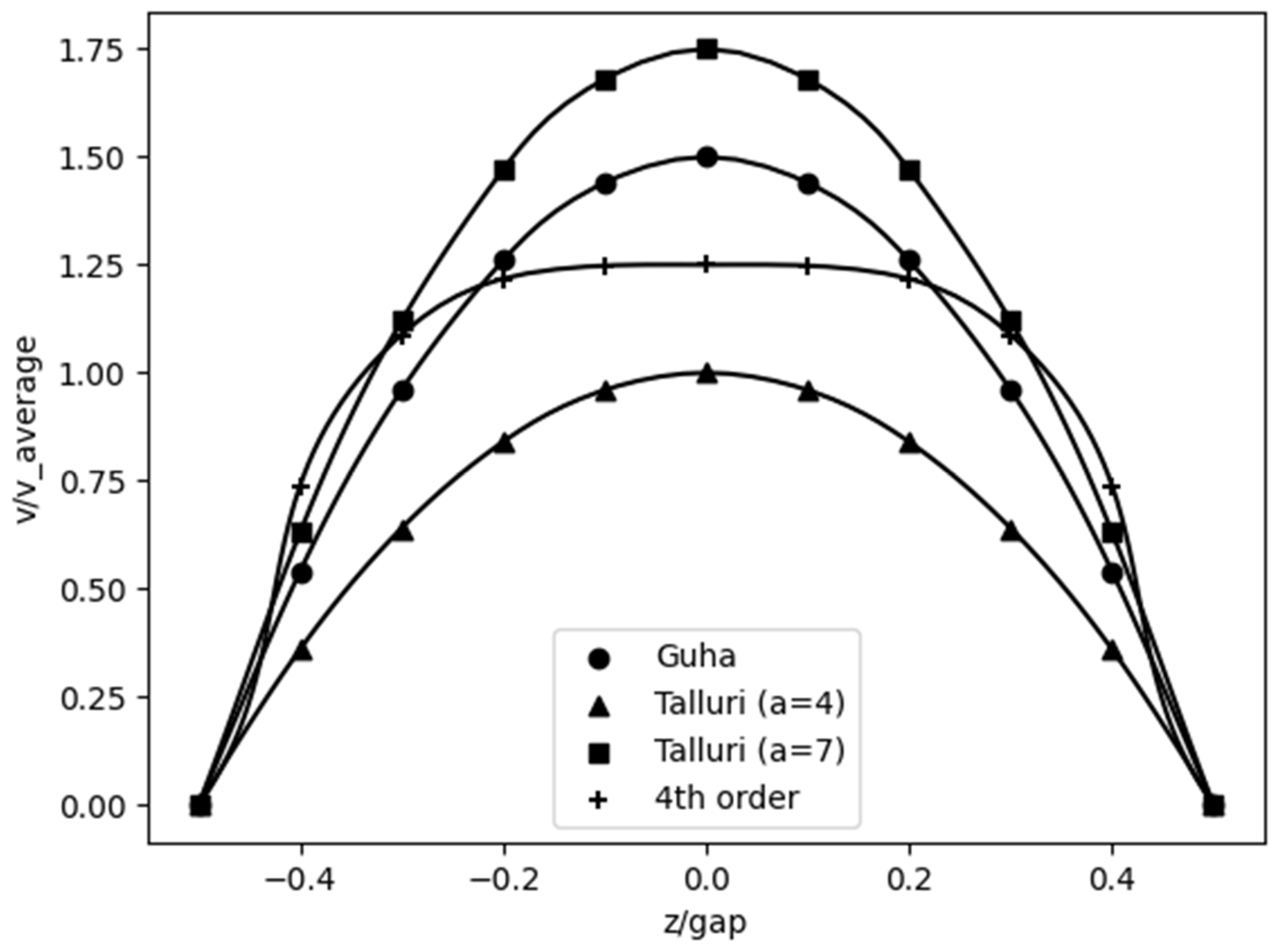
The solution to the derived form of the Navier–Stokes equations with the simplifications requires the prescription of the velocity profiles in the rz-plane of the gaps between the disks. A no-slip condition is specified in the disk walls. Of the several possible velocity profiles that are found in the literature for generic solutions of this form, three of them that were hypothesised to capture the flow within the channels of Tesla pumps were explored in this work. Initially, a modified version of the baseline velocity profile from the recent work by Guha and Sengupta [30] were applied and, thereafter, in a bid to improve the accuracy of the results, alternate forms of the velocity profiles, including the baseline profiles, were tried out. These are described below:
- Guha and Sengupta [30]:
According to this approach, the velocity profiles are considered parabolic for fully developed flow. The expressions are:
where and are the average radial and tangential velocities in z direction, respectively.
Setting z = 0 in the middle of the gap, z = ±½ in the wall boundaries and integrating the Navier–Stokes equations results in the equations below:
Momentum conservation in the radial direction:
Momentum conservation in the tangential direction:
- Talluri
Improving on the previous approach, Talluri added a factor “a” in the parabolic profile. Factor “a” is not constant, as lower values indicate not fully developed flow and should be near the inlet, whereas higher values indicate fully developed flow and should be near the outlet. Integrating the Navier–Stokes equations between z = 0 and z = b/2 gives:
Momentum conservation in the radial direction:
Momentum conservation in the tangential direction:
Talluri conducted a parametric analysis to evaluate the factor “a” that produces the model profiles that best fit the real profiles. The best approach is a radius-dependent factor “a”, so that it can be different for undeveloped and developed flows. Talluri’s suggestion is that factor “a” is equal to 4 for undeveloped flow near the inlet after comparison with the CFD results for the working fluids R404a, R134a, R245fa and R1233zd(E) [28]. For fully developed flow, “a” is equal to 8, as suggested by [31] after validation with the CFD results. In the present work, the factor “a” is equal to 4 if the distance covered by the fluid is less than the entry length for developed flow and equal to 7 otherwise.
- Schosser, 4th order model [32]
Schosser proposed a 4th degree polynomial to express the velocity profile. Following this proposition, a velocity profile that is hypothesised to provide similar representation with additional local flexibility and control in the profile shape is as worked out below:
Similar to the previous approaches, the integration of the Navier–Stokes equations results in the next equations:
Momentum conservation in the radial direction:
Momentum conservation in the tangential direction:
Figure 2 presents the velocity profiles together for comparison. The axial distance is normalised over the gap and the velocity over the average velocity. These velocity profiles are intended to represent the flow through the entire rotor channel. Seemingly, it is here that there exists a designer’s choice to implement the extent of “peakedness” or kurtosis to represent the nature of the wall shear action on the flow within the channels. These profiles indicate three different possible approaches: 1. Guha and Sengupta’s profile assumes a single parabolic profile as sufficient over the entire rotor; 2. Talluri’s profile assumes a radial correction is required to mimic the development of the flow as the radius increases; and 3. Schosser’s profile indicates a departure from the parabolic modelling and proposes a flatter profile as a reasonable compromise to account for the different regimes. In addition to the profiles considered here, several radius-based corrections that include the effect of separation and the consequent inflection have been tried. However, in this simple 1D design code, such detail is considered unwarranted. The validity of this simple modelling can be ascertained via the discussion of the results with these simple profiles in the next section.
3. Results
3.1. Main Code Results
The solutions to the derived Navier–Stokes equations with the volute loss model and velocity profiles are discussed in this section. Initially, the solutions are generated with Talluri’s velocity profile in order to explore the validity of the volute loss modelling.
The solution is generated for the Morris pump design that was experimentally characterised. The key geometric and inlet conditions of the reference experimental case are summarised in Table 1 and Table 2. It is noted that after the rotor, the flow enters five diffuser channels with an expansion angle of 7.6°. The diffuser is followed by a volute with a logarithmical spiral shape and then a conical diffuser with an 8° expansion angle.
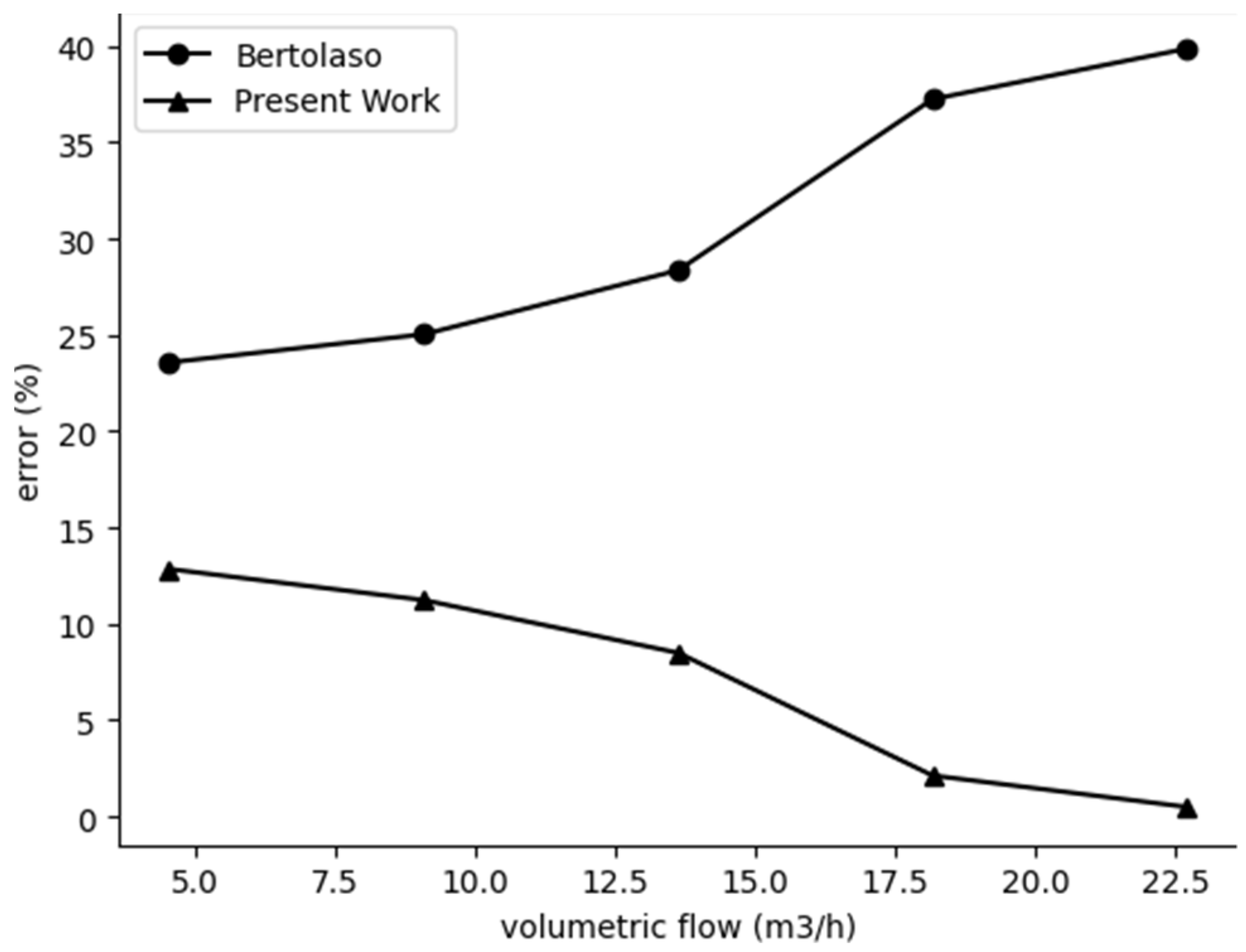
The comparison of the results for the Morris pump geometry with the updated version of the loss model with the baseline corrections for the volute model in Bertοlaso’s work is shown in Figure 3 indicatively for the case of a 6000 rpm rotational speed and a 25.4 mm internal diameter. The error in the pump outlet static pressure with the update in the volute loss model over the entire mass flow range has reduced from the range of 24–40% to 1–13%. Moreover, the updated physics-based model performs better near the design mass flow rates from 15 to 20 m3/h. The significant improvement obtained via the correct implementation of a volute loss model is a noteworthy improvement for the 1D design code. The opposite trend of the two curves in Figure 3 is attributed to the following major corrections on previous work: the number of the gaps is set as the number of the disks minus 1, the velocity in Equation (10) is raised to the second power, the coefficient in Equation (13) is set to 0.5, and the missing density factor is added to Equations (11) and (12).
The present 1D design code with the improved volute loss modelling is then used to simulate the complete range of flow rates and shaft speeds, as in Table 2. The results of the code are compared with the experiments with the main parameter of interest, which is the static pressure at the rotor and the pump outlet. Both these static pressure measurements are available from the experimental data and are, in essence, the key metrics of the pump design. The error between the model results and the experimental results is calculated using the formula below:
The quoted average error corresponds to the average of all the operating cases and is calculated by:
where n is the number of the operating cases tested.
The average errors of the static pressure at the rotor and pump outlet of all the operating cases are shown in Table 3.
It is observed from Table 3 that even though the rotor outlet static pressure indicates an average error of 3%, the average error at the pump outlet is more than 11%. It is in an attempt to improve this error at the pump outlet that different velocity profiles, as explained in the previous section, are tested, with the results shown in the next section.
3.2. Results after Applying the Different Velocity Profiles
The results of the 1D design code with different velocity profiles are compared to the experimental data. The static pressure error averages of all the operating cases are shown in Table 4.
The following is observed from the error after implementation of the velocity profiles:
- The velocity profiles that include a radius correction using Talluri’s approach can predict values closer to the experimental data for the rotor outlet static pressure. An error of less than 5% at the rotor exit is deemed satisfactory for the purposes of the pre-detailed design sizing code and, therefore, the use of further complicated velocity profiles to obtain further improvements, if any are possible at all, is deemed unnecessary.
- In all the approaches, the error at the rotor is less than the error at the overall machine. Therefore, the main cause of the difference from the experimental results is likely to be the modelling of the outlet. Irrespective of the choice of velocity profile, the average error at the pump outlet is still more than 10%.
4. CFD Analysis of the Rotor
4.1. Simulation Parameters
The results derived from the 1D design code indicate that averaged errors of more than 10% for the complete pump operating flow and speed range are observed in the pump outlet static pressure. However, the average errors for the rotor outlet static pressure are only 3% with the Talluri’s model, which has a radius-based correction implemented in the code. Moreover, the inclusion of the physics-based loss model for the outlet volute produced a significant improvement in the errors compared to the previous implementations of Bertοlaso’s model in a fixed speed line, with the mass flow average shifting nearly 30% to around 10%. Therefore, improvements in the modelling of the overall pump outlet static pressure are possible by further refining the outlet volute modelling. However, the prediction of the volute loss depends on the accuracy of the flow field variables at the rotor outlet. Consequently, it is decided that a 3D RANS solution for the flow in the inter-disk gap of the rotor will provide additional information on the flow field variables for subsequent volute loss modelling by resolving the realistic flow phenomena without the limiting assumptions of axisymmetric flow, as in the 1D design code.
Moreover, it is emphasised that this exploration of the detailed flow field within the inter-disk gap is not attempted in a bid to improve the velocity profile modelling as is traditionally attempted in the literature, because the radius-corrected velocity profiles already provide a good prediction of the rotor outlet static pressure. Instead, the 3D RANS analysis in the inter-disk gap serves two purposes. First, to identify the realistic rotor flow field development with fewer assumptions and compare the resultant rotor outlet pressure with experiments. This would provide a means to identify the extent of the improvement, if any, over the 1D design code that is possible by including the most realistic circumferentially and radially varying the resolved flow field. Second, to provide information on various additional considerations arising from the rotor outlet flow field that would subsequently develop further in the volute and impact the losses. A description of such phenomena would pave the way for future researchers to suitably propose improved volute loss models, which will successfully close the gap in the pump outlet static pressure error predictions.
The 3D RANS solutions were obtained using a commercial implementation of a finite-element-based finite volume solver, ANSYS CFX [33]. Higher-order resolution schemes for advection were used to minimise the numerical truncation errors. The turbulence closure was modelled using two-equation turbulence models for the turbulence kinetic energy (k) and turbulence dissipation rate (ω). The near wall flow physics is explicitly resolved by ensuring a y+ value of less than 1 because of the importance of the wall shear resolution in transferring energy to the flow in the small inter-disk gap.
The following two cases were examined:
- Case A: shares the same geometrical dimensions and boundary conditions with Morris’ experimental studies with a gap size of 0.152 mm.
- Case B: the same geometry as Case A but with the gap set as 0.889 mm. This was done to identify if the inter-disk gap change has any significant impact on the flow field development, which would influence the rotor outlet–volute channel inlet flux features. The dimensions in the experimental study were originally in inches. The cases with gaps of 0.006 in. and 0.035 in. were converted into 0.152 mm and 0.889 mm, respectively; hence, the numbers are not round.
The modelled domain of interest was a single gap between two rotating disks. Two extensions were added to the domain to avoid border inaccuracies and ensure developed flow at the inlet: a ring of +25% radial space at both the inlet and the outlet. This resulted in three domains in total.
The computational domain was discretised using a commercial grid generation package, ANSYS ICEM CFD [34]. A structured non-orthogonal, hexahedral body-fitted grid topology was selected to ensure the appropriate resolution of flow features with similar levels of flow resolution in an area-expanding radial outflow channel geometry. All the grid elements were ensured to have a skewness angle in the range of 30 to 150 degrees, aspect ratios of less than 100 and expansion ratios of less than 1.2 to meet the typical best practice guidelines for finite volume solvers and avoid flux interpolation errors.
Each of the three domains were discretised separately so that it was possible to have different numbers of nodes at the circumferential direction as the radius changed. The domains were connected using general grid interfaces that did not require restrictive one-to-one connectivity while ensuring appropriate transfer interface fluxes. The flow inside a gap was mainly dictated by boundary layer physics. No mesh independence study was conducted because the literature suggests that y+ values less than or equal to 1 provide sufficient mesh quality for boundary layer modelling [35]. Thus, the selection of the node number within the inter-disk gap was mainly affected by the fact that at least a minimum of 10 nodes in the smaller gap case and 20 nodes in the larger gap case were required in the axial direction to keep the first near wall node elements well within the y+ upper limit of 1. The number of nodes in each circumferential edge at different constant radii and the number of nodes in radial edge that passes through the circumferential edges were finalised after a focused grid sensitivity study on the parameters of interest. The numbers of nodes in both the circumferential and radial edges were chosen with the constraint on the aspect ratios that is within the best practice guidelines. The final grid parameters are shown in Table 5 below.
It is observed that even though Case B has a larger gap, it is modelled with less total nodes than Case A. The large gap, however, is discretised by twice as many axial nodes as those in Case A and, thus, the y+ ≤ 1 criterion is satisfied.
The fluid domains were considered to be stationary, and the rotor walls were considered to be rotating. This method reduced the uncertainties associated with solving the rotating frame of reference equations in the stationary inter-disk space. The wall boundary conditions were rotating no-slip for the rotor domain and stationary free-slip for the inlet and outlet ring. Free-slip conditions were specified in the inner and outer rings because they are numerical constructs required to pre-condition the flow and transfer the far field outlet boundary condition into the rotor outlet. Therefore, there is no physical or numerical requirement for the flow in these domains to be affected by the numerical end walls. All the walls were considered adiabatic. At the inlet conditions, the fluid had a total pressure of 446 kPa, a total temperature of 52.5 °C, the flow was subsonic, and the velocity had a radial direction. At the outlet, the mass flow was set as the experimental total flow divided by the number of gaps, since one gap is simulated. This was chosen as one of the experimental points from the Morris pump under investigation in the 1D design code as well.
The steady-state Reynolds-averaged Navier–Stokes (RANS) equations were solved. The k-ω Shear Stress Transport model was chosen for the regions close to the walls, whereas the k-ε model was chosen for the regions away from the walls [35], following the typical blended turbulence resolution approach whereby models that perform well in the respective regions are chosen. The turbulence intensity was set to 1% and the solution of the total energy equation was enabled. In total, 32 experimental cases of Morris were run as simulations in the “Crescent” HPC facility of Cranfield University using a parallelisation scheme over 2 chunks of 16 CPUs. The duration of each simulation was 2 h for Case A and 1 h for Case B.
4.2. Velocity Profile Results
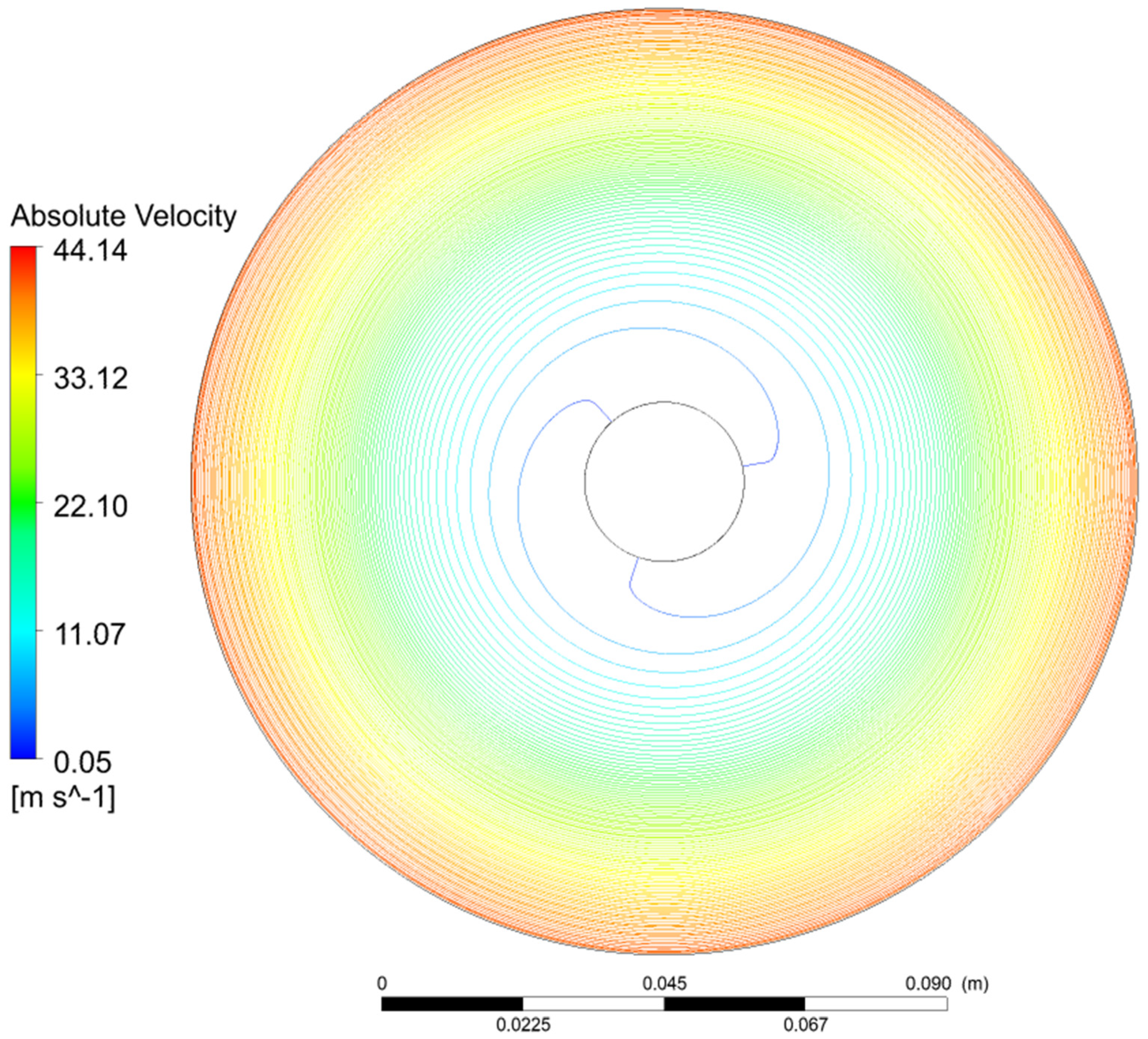
In this section, the results of the simulations are discussed. It is noted that the CFD was not used for the validation of the 1D code, which was previously validated based on the experimental data. The 1D code is concerned with a model of a whole pump, whereas the CFD fluid domain is limited to a single inter-disk gap, so that it gives insight into the flow details inside the rotor. The experimental work of Morris mainly evaluates the performance of the pump and does not provide flow details. The general flow field in the rotor is illustrated by considering Case B with a 6000 rpm rotational speed and an 18.17 m3/h flow rate. The flow field for Case A is also similar, albeit with differences in the magnitude of the phenomena; therefore, one of the cases is chosen to describe the general flow field. The differences in terms of the velocity profiles between the cases are described subsequently. Figure 4 below shows the absolute velocity streamlines at the rotor at the midplane between two disks. It is observed that the velocity is radial at the inlet and then follows a spiral trajectory due to the frictional and centrifugal forces. The acceleration of the absolute velocity is driven by the work transfer due to the wall shear and the increased rotational velocity with the increase in the radius. Figure 5 illustrates the static pressure contour from the inlet to the outlet. The static pressure increase corresponds to the work input and the energy transfer from the rotating disk to the fluid.
The results indicate the expected increase in the velocity and pressure as the radius increases as more energy is transferred to the fluid through the frictional forces.
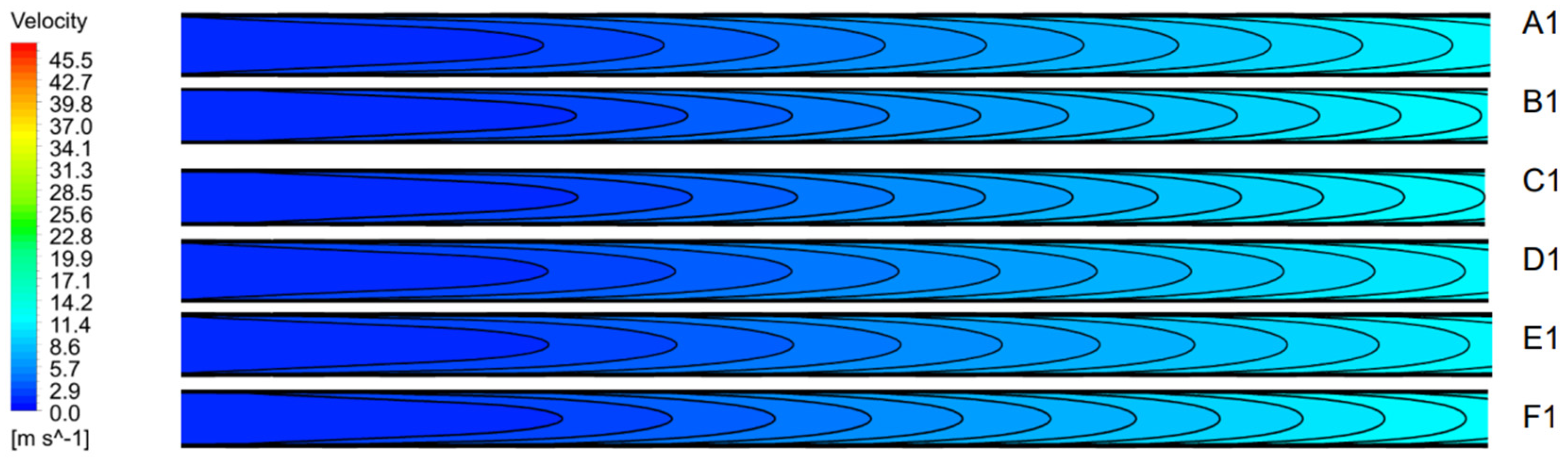
In order to capture the velocity profiles at the gap, the rotor domain is intersected by six semiplanes named using the letters from A to F. The progression of the semiplane is defined by the axis of rotation and the radial direction. The angle between two consecutive semiplanes is 60°, as shown in Figure 6. Each semiplane is divided in the radial direction into three regions of equal radial space, which are numbered from 1 to 3: the inlet, the middle and the outlet.
Each planar section is named with the letter of the semiplane it belongs to followed by the number of the region.
The velocity profiles at the inlet and outlet regions at each of the six semiplanes are illustrated in the images below. The radius increases from the left to the right.
It is observed in Figure 7 and Figure 8 that as the flow moves towards the outlet, the velocity profiles gradually lose their parabolic shape, flatten and a flow inversion is detected near the outlet. Figure 9 below shows the streamlines and the profile in the F3 area in more detail. F3 is the outlet of the rotor, and it is in the inlet of the volute channel.
It is observed that there is a recirculation zone near the outlet that causes the inversion of the velocity profile. Part of the energy transferred to the fluid is consumed in this recirculation area, causing losses near the outlet to be convected down into the volute channel. The separation zone at the outlet is observed to have a wavy nature around the circumference, with peaks and troughs in the extent of the velocity inversion. A similar flow field inversion with different magnitudes of absolute velocity and extents of inversion is observed in the smaller gap in Case A.
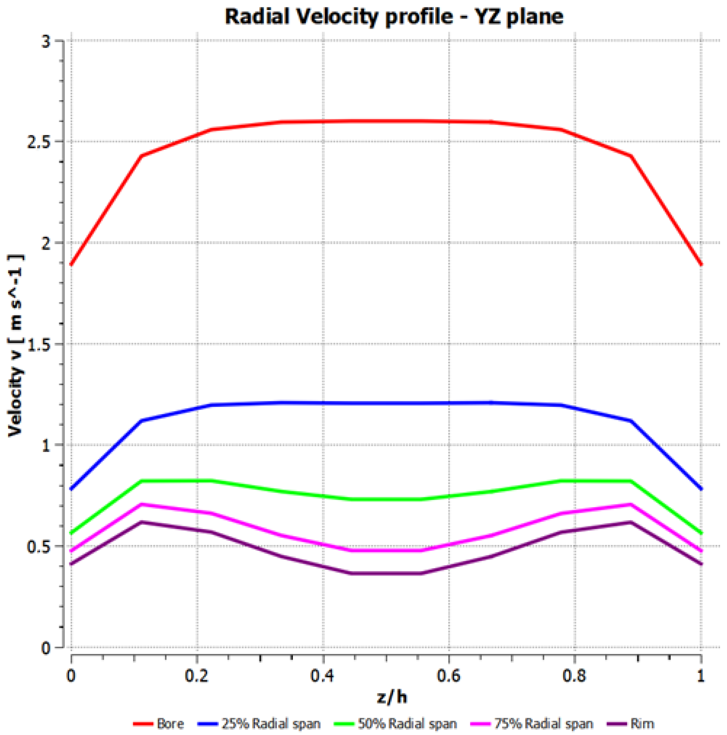
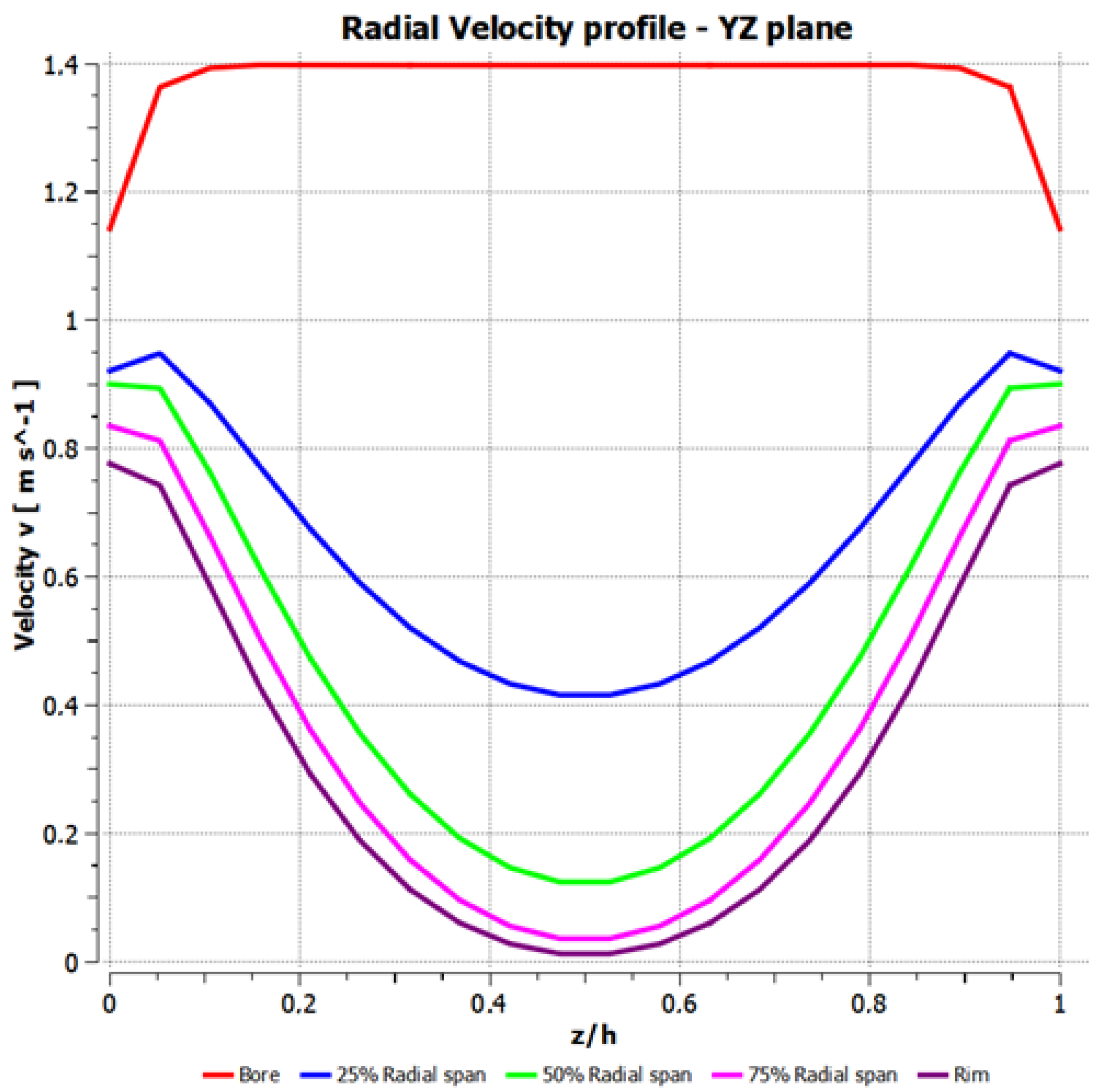
The circumferentially averaged radial velocity profiles plotted at different radial locations along the channel indicate the development of the flow inversion. These radial velocity profiles are shown in Figure 10 and Figure 11 for Case A and Case B, respectively. The magnitude of the radial velocities is higher in the smaller gap in Case A because of the stream-tube contraction in the smaller inter-disk gap. Consequent on this higher gap, the extent of the peak inversion is lower in Case A than Case B.
In Case A, it is noted that the extent of the positive kurtosis–peakedness within the inter-disk gap is reducing with an increase in the radius. At about a 50% radial location, the kurtosis has disappeared and there is a flat radial velocity profile. Beyond a 50% radial location, the negative kurtosis of the radial velocity profile increases with the radius. At the rim, a characteristic “M”-shaped profile develops. The “M” profile is formed because the transfer of the energy from the disks still affects the fluid in the near vicinity of the rotating walls. However, in the middle region, the flow inversion causes a sharp drop in the radial velocity profile from both the rotating wall ends.
In Case B, it is observed that the decreasing trend of the positive kurtosis reaches a flat profile within the first 10% of the radius. Thereafter, the negative kurtosis progressively increases to the rim. The extent of the inversion is significantly higher than that in Case A because of the lower magnitude of the velocities in this larger gap case. At the outlet, the extent of the rotating walls, which causes the peaks of the “M” profile, is reduced by half when compared to Case A. Subsequently, at higher radial locations, the inversion occupies nearly the complete inter-disk gap. Thus, the extension of the inversion through the disk gap results in the formation of a characteristic “U”-shaped profile.
Therefore, the recirculation zone that forms at the rotor outlet–volute inlet region due to the adverse pressure gradient is found to significantly influence the radial velocity profiles in the inter-disk gap. The radial velocity profile within the inter-disk gap can, in reality, vary from anywhere between a typically assumed parabolic profile with positive kurtosis to a completely inverted “U”-shaped profile with negative kurtosis through flat and “M”-shaped profiles.
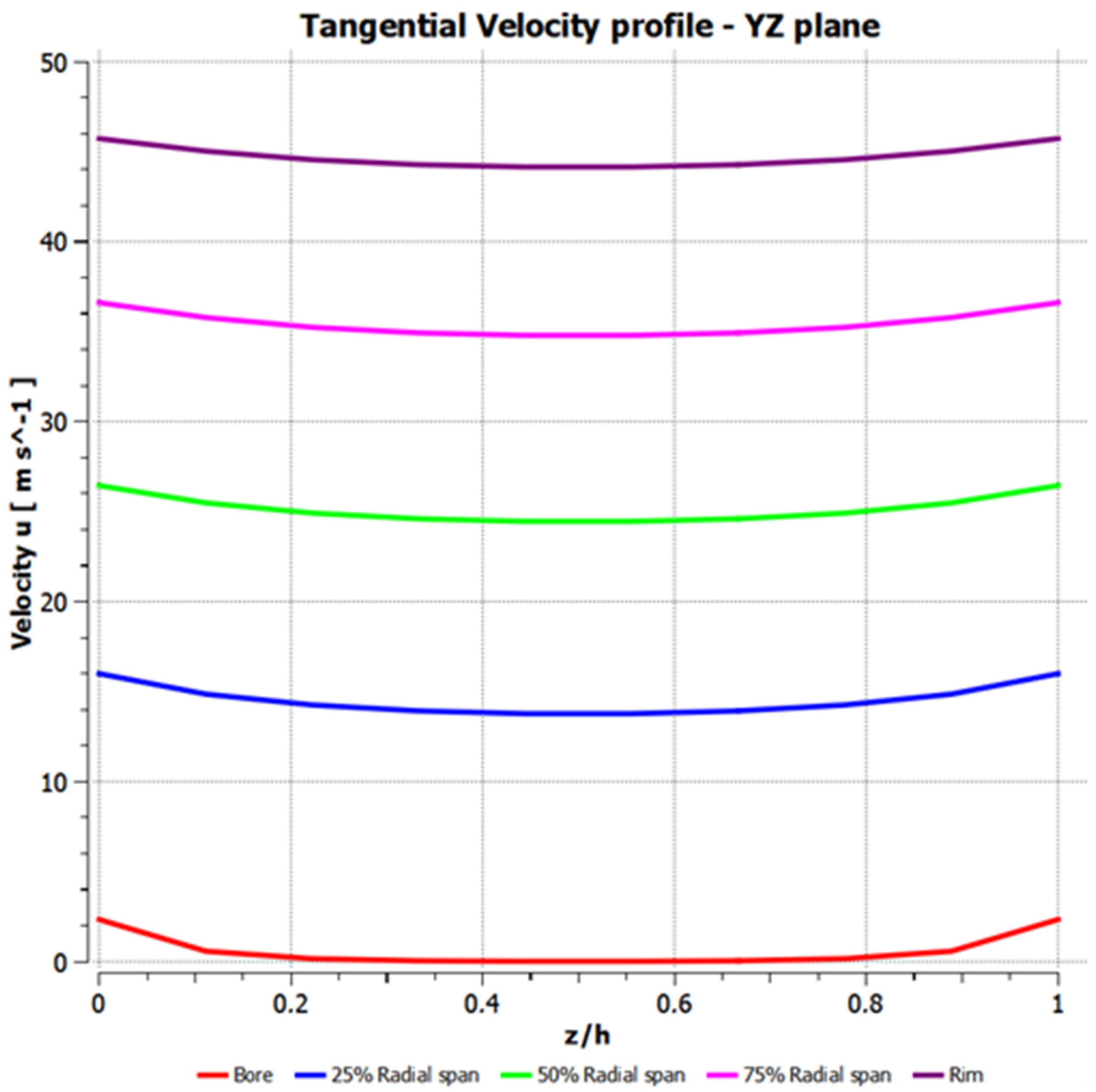
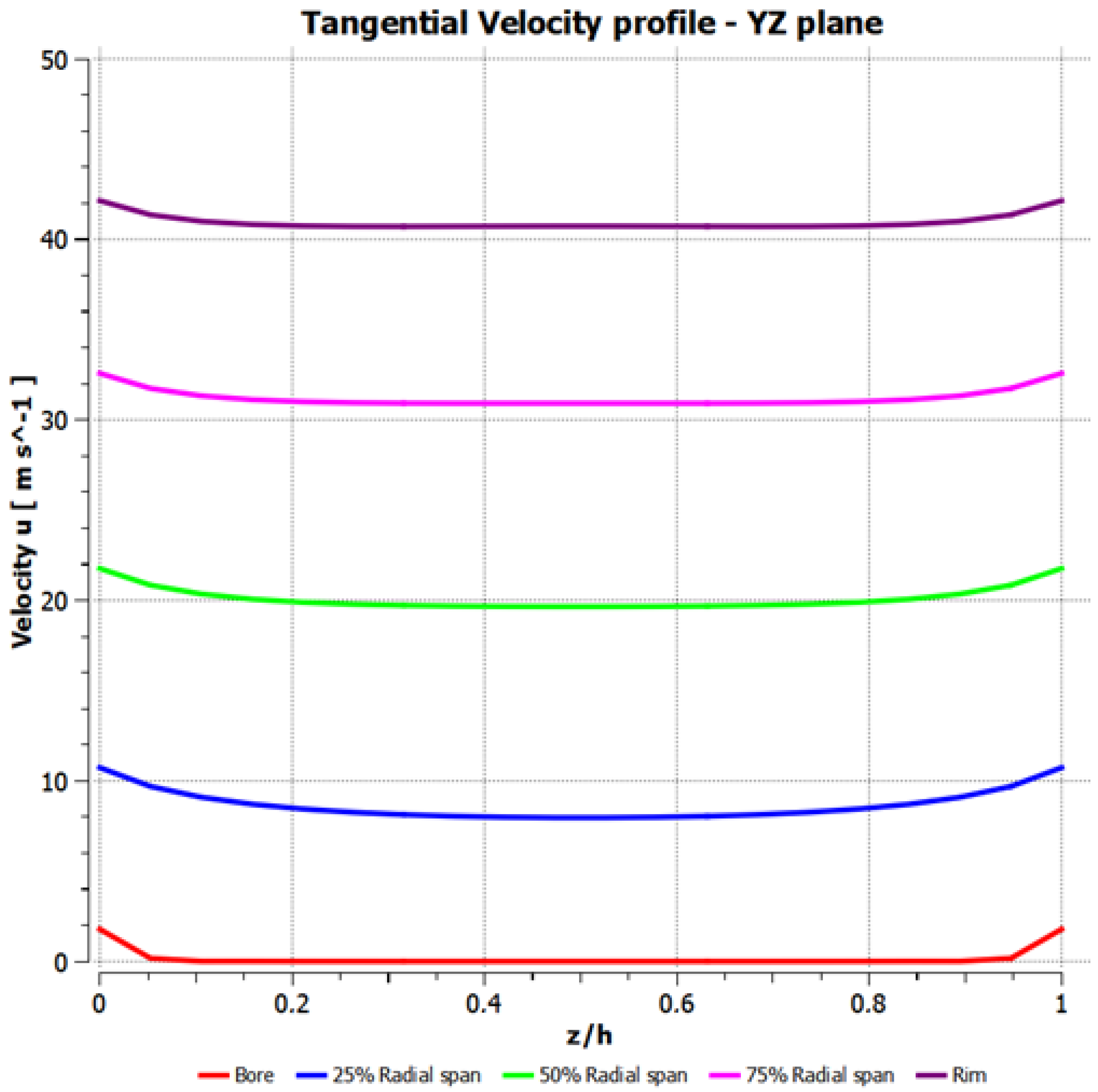
The tangential velocity profiles for Cases A and B in the inter-disk gap are shown in Figure 12 and Figure 13. The tangential velocity profiles increase from the bore to the rim following an increase in the blade speed. Minor drops are observed between the rotating end walls and the bulk fluid, which are representative of losses in the energy transmission through the wall shear. As in the previous case, the magnitude of the tangential velocity is lower in Case B than Case A due to the stream tube contraction-driven velocity increase in the smaller gap. This tangential velocity uniformity and radial increase is expected because of the lower pressure gradients in the circumferential direction at a fixed radius.
4.3. Characteristic Curves and Volute Losses
To compare the CFD results with the experimental data in terms of the pump performance, the characteristic curves in terms of the pressure ratio for different mass flow rates are generated for Case A and B at a rotational speed of 6000 rpm, which is the design speed of the pump. Figure 14 shows the total pressure ratio plotted for both cases from the experiments and simulations. The experimental pressure ratios correspond to the overall pump outlet, while the pressure ratios from the simulations correspond to the rotor outlet, which explains the difference between the curves. The characteristic curves traditionally have the total pressure to the y-axis, and the static pressure follows the same trends. Interestingly, it is observed that the experimental characteristic curves are not different for both the cases of different disk gaps. However, the rotor-only simulation-generated curves exhibit a nearly 15% difference between the two cases. This is because, in Case B, the rotor total pressure ratio is lower than in Case A for the same flow rate. Therefore, it is to be expected that the overall losses in the components other than the rotor is more for Case A than Case B to bridge the difference in the pressure ratios.
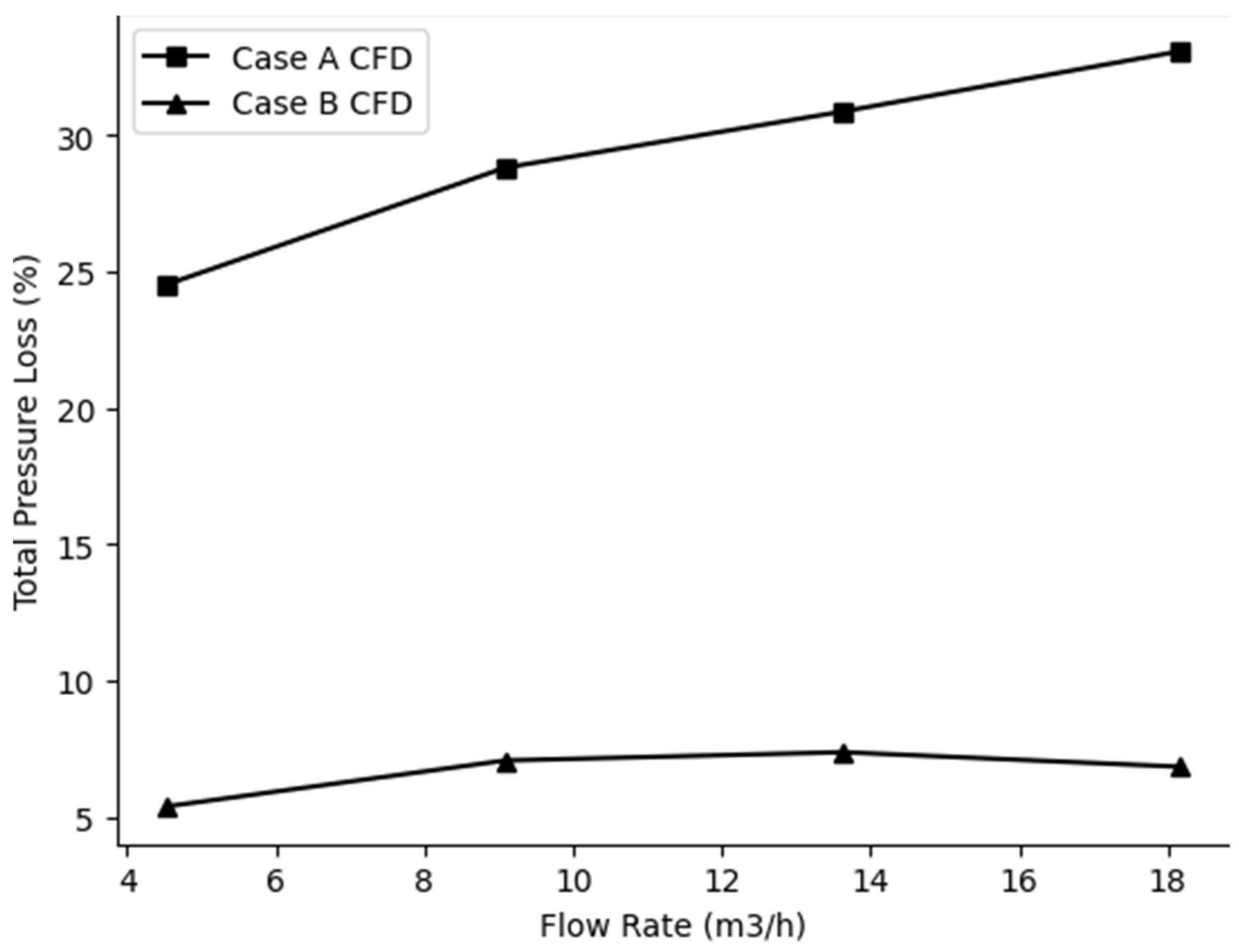
The total difference between the rotor-only simulation results and the experiments are shown in Figure 15. In addition to the numerical and experimental uncertainties, the differences are completely attributable to the losses in the volute collector and the intake region. However, since the intake region involves low velocities and does not have any significant loss-generating flow mechanism or feature, most of these losses are attributable to the volute collector. The extent of these losses in the volute is in the range of 25–33% for Case A and in the range of 5–8% for Case B.
Herein lies the challenge in the modelling of the volute losses for the Tesla pump. The general trend noticed in the higher losses for the smaller gap in Case A than the larger gap in Case B is consistent with the flow physics-based expectation that the larger radial and tangential velocities would lead to higher losses. However, just the difference in the magnitude of the velocities is not sufficient to explain the difference in the losses. Therefore, it is suggested that additional variables associated with the variation in the flow field properties at the exit of the rotor would need to be considered in the volute loss modelling. This differs significantly between the cases considered and, in general, can vary anywhere between a traditional parabolic profile and a completely inflected “U”-type profile, with several variations of “M”-shaped profiles in between. Therefore, it is suggested that to have an appropriate resolution to the volute losses, at least a higher fidelity loss model that would account for additional variables related to the velocity profiles at the rotor outlet is required.
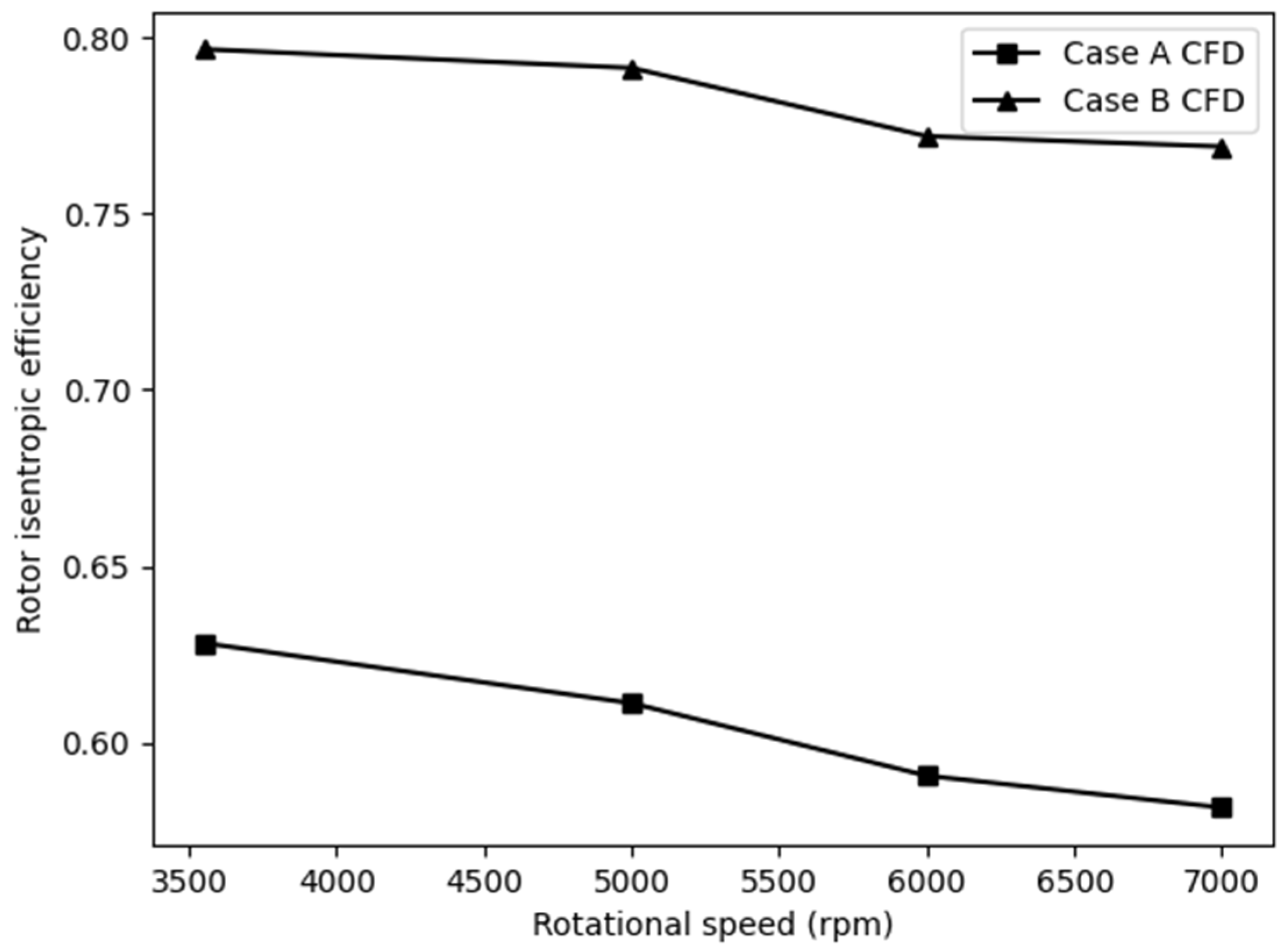
This observation is further bolstered by the fact that a complete characterisation of the rotor only indicates high efficiencies across different rotational speeds and at different flow rates for a fixed rotational speed. Figure 16 illustrates the rotor isentropic efficiency for different rotational speeds at a constant flow rate of 13.63 m3/h, which is the design point and equal to 60 gallons per minute in the original experimental report. The curves follow similar trends for the flow rates of 4.54 m3/h (20 gallons per minute) and 9.08 m3/h (40 gallons per minute), as seen in Figure 17 and Figure 18. Figure 19 illustrates the rotor isentropic efficiency at a constant 6000 rpm for different flow rates. Similar curves can be seen in Figure 20 and Figure 21 for a constant 3550 rpm and 7000 rpm, respectively. These plots indicate that the rotor efficiencies in Case A are greater than in Case B for the whole operating speed range and in most of the mass flow range, except at low mass flow rates. Furthermore, it can be observed that the low efficiency in the rotor is coupled with a lower loss in the volute. This is consistent with the physical observation that the lower efficiency in the rotor corresponds to the differences arising due to the same work addition resulting in a lower pressure rise and absolute velocity. The lower absolute velocity qualitatively explains the lower volute loss in consequence. Therefore, a careful optimisation in the breakdown of the losses between the rotor and the volute could hold the key to the improvement of the efficiencies of Tesla pumps. Such improvements are linked to the development of a better higher-resolution loss model for the volute. This is particularly because, irrespective of the significant assumptions involved in the rotor velocity profiles in the 1D design codes, these codes are still able to predict the rotor-only performance as well as the CFD solutions.
5. Conclusions
An axisymmetric 1D design code that can be used for the sizing of Tesla pumps is adapted from the Q1D numerical tool developed by Talluri [8] by considering physics-based models for each of the components. A simplified adiabatic intake model is used to compute the flow properties at the inlet of the rotor stack inter-disk gap. The rotor model in the code solves the axisymmetric Navier–Stokes equations in cylindrical co-ordinates by considering a choice of velocity profiles in the rz-plane that is representative of the inter-disk gap in the Tesla pump rotor stack. A flow-physics-based loss model that computes the friction losses in the volute based on the kinetic energy coefficients that are derived from centrifugal pumps is used with updates from a simpler version with baseline coefficients. The results derived from the code are compared with one of the water pumps in the experiments conducted by Morris [26]. After an exploration of different choices of velocity profiles for reducing the Navier–Stokes equations, it is noted that velocity profiles that include radius corrections yield an average error of around 3% in the rotor outlet static pressure over the entre operating range compared to the experimental data. The radius-corrected velocity profiles perform better than the typical parabolic and higher-order velocity profiles. However, the overall pump outlet static pressure indicates an average error of around 10% over the entire operating range.
Therefore, 3D RANS solutions of the rotor inter-disk gap are conducted to provide the resolution on the rotor flow field to identify the flow field features without the axisymmetric and velocity profile assumptions and appropriately provide directions for the improvement of the volute loss model. Two cases with different inter-disk gaps are simulated and compared with the experimental results. The details of the general flow field that include the development of inflection in the velocity profiles from typical parabolic profiles to yield characteristic “M”-shaped and “U”-shaped profiles are described as in other detailed studies of Tesla pumps. An additional circumferential waviness that is associated with the inflection influenced outflow is also observed at the rotor outlet. The results obtained from the characterisation of the rotor performance from the 3D RANS solutions are in a similar error band to the 1D design code. Therefore, the axisymmetric assumption in the rotor with a radius-based velocity profile correction, even without accounting for a family of inflected profiles, is deemed satisfactory for a 1D design code. However, detailed comparisons of the rotor-only simulations with the overall pump performance indicate that the major portion of which the discrepancies with regard to the experimental data is attributable to the volute losses varying in the range of 25% to 33% for the lower inter-disk gap and 5% to 8% for the higher inter-disk gap. The reduction in the magnitude of the absolute velocity with the increase in inter-disk gap is not sufficient to bridge the difference in the losses, as will be the case in the typical volute loss models used in the literature and in this study. Therefore, it is suggested that the volute model in the 1D design code would need to be expanded to include additional considerations from the flow field at the rotor outlet, which includes the radial inflections and circumferential waviness.
The guidelines deduced in this study are distinct from previous efforts described in the literature, in which detailed 3D RANS studies were used to improve the velocity profiles in the rotor. On the contrary, this study notes that the improvement in the velocity profiles achieved by including realistic velocity profiles does not contribute as much to improving the accuracy of the 1D design code as using the realistic flow fields to improve the loss modelling in the volute. This is proven by the ability of the code described in this work and in other published works to predict rotor-only performance within a 5% error band.
Moreover, a lower efficiency in the rotor was found to correspond with a lower loss in the volute. Therefore, a careful development of the volute loss model would provide the means to identify an overall pump that would have a high efficiency rather than having a rotor of high efficiency that is coupled with a high loss volute. The achievement of such an improved 1D design code with an improved loss model for the volute, as is considered in a future extension of this work, would pave the way for understanding the performance of existing geometries and provide the capability to develop bespoke Tesla pump designs with the required levels of efficiency for aircraft thermal management applications.
Author Contributions
Conceptualization, D.J.R. and E.A.P.; software, R.F., D.J.R. and L.T.; validation, E.A.P.; formal analysis, D.J.R. and R.F.; investigation, R.F., A.B., D.J.R. and E.A.P.; resources, D.J.R. and L.T.; data curation, R.F. and A.B.; writing—original draft preparation, A.B. and D.J.R.; writing—review and editing, D.J.R. and I.R.; visualization, R.F. and D.J.R.; supervision, E.A.P. and I.R.; project administration, I.R.; funding acquisition, Not applicable. All authors have read and agreed to the published version of the manuscript.
Funding
This research received no external funding.
Data Availability Statement
No new data were created or analyzed in this study. Data sharing is not applicable to this article.
Conflicts of Interest
The authors declare no conflict of interest.
Nomenclature
| Absolute velocity at the inlet of the rotor | |
| Mass flow | |
| Density | |
| Internal diameter at the bore of the disk | |
| Gap space between two consecutive disks | |
| Static pressure at the tank | |
| Static pressure at the inlet of the rotor | |
| Absolute velocity | |
| Relative velocity | |
| Radial component of absolute velocity | |
| Tangential component of absolute velocity | |
| Radial component of relative velocity | |
| Tangential component of relative velocity | |
| Axial component of absolute velocity | |
| Axial component of relative velocity | |
| Rotational speed | |
| Radial position | |
| Axial position | |
| Pressure drop at the inlet of the diffuser | |
| Absolute velocity at the exit of the rotor | |
| Pressure drop at the outlet of the diffuser | |
| Absolute velocity at the inlet of the diffuser | |
| Absolute velocity at the exit of the diffuser | |
| Pressure drop at the cone outlet | |
| Absolute velocity at the exit of the throat | |
| Absolute velocity at the exit of the cone | |
| Tangential velocity dump losses | |
| Tangential component of absolute velocity at the exit of the rotor | |
| Radius at the tongue of the volute | |
| Radius at the throat of the volute | |
| Volute angle | |
| Friction factor | |
| Length of the spiral of the volute | |
| Friction losses | |
| Average velocity in the volute | |
| Static pressure as calculated by the present work | |
| Static pressure from experimental data |
References
- Newbury, S. Aerospace Technology Institute—FlyZero Academic Programme Research Findings and Recommendations, Report FZO-ACA-REP-0056; Department for Business, Energy, & Industrial Strategy: London, UK, 2022.
- Tesla, N. Fluid Propulsion, USA. Available online: https://teslauniverse.com/nikola-tesla/patents/us-patent-1061142-fluid-propulsion (accessed on 22 June 2022).
- Truman, C.R.; Rice, W.; Jankowski, D.F. Laminar through flow of a fluid containing particles between corotating disks. ASME J. Fluids Eng. 1979, 100, 87–92. [Google Scholar] [CrossRef]
- Pacello, J.; Hanas, P. Disc Pump-Type Pump Technology for Hardto-Pump Applications. In Proceedings of the 17th International Pump Users Symposium; Texas A&M University: College Station, TX, USA, 2000. [Google Scholar]
- Medvitz, R.B.; Boger, D.A.; Izraelev, V.; Rosenberg, G.; Paterson, E.G. CFD Design and Analysis of a Passively Suspended Tesla Pump Left Ventricular Asis Device. Artif. Organs 2011, 35, 522–533. [Google Scholar] [CrossRef] [PubMed]
- Yu, H. Flow Design Optimization of Blood Pumps Considering Hemolysis. Doctor of Engineering; Magdeburg University: Magdeburg, Germany, 2015. [Google Scholar]
- Hasinger, S.H.; Kehrt, L.G.; Goksol, O.T. Cavitation tests with a high efficiency shear force pump. In Proceedings of the ASME Symposium on Cavitation in Fluid Machinery, Chicago, IL, USA, 7–11 November 1965; pp. 132–147. [Google Scholar]
- Anselmi, E.P.; Fiaschi, D.; Manfrida, G.; Nicotra, G.; Talluri, L. Design and Optimisation of a Tesla Pump for ORC. In Proceedings of the 6th International Seminar on ORC Power Systems, Munich, Germany, 11–13 October 2021. [Google Scholar]
- Sengupta, S.; Guha, A. A non-dimensional study of the flow through co-rotating discs and performance optimization of a Tesla disc turbine. SAGE J. Power Energy 2017, 231, 721–738. [Google Scholar] [CrossRef]
- Song, J.; Ren, X.; Li, X.; Gu, C.; Zhang, M. One-dimensional model analysis and performance assessment of Tesla turbine. Appl. Therm. Eng. 2018, 134, 546–554. [Google Scholar] [CrossRef]
- Schosser, C.; Lecheler, S.; Pfitzner, M. Analytical and Numerical Solutions of the Rotor Flow in Tesla Turbines. Period. Polytech. Mech. Eng. 2017, 61, 12–22. [Google Scholar] [CrossRef]
- Rusin, K.; Wroblewski, W.; Rulik, S. Efficiency based optimization of a tesla turbine. Energy 2021, 236, 121–448. [Google Scholar] [CrossRef]
- Alonso, D.H.; de Sa Nogueira, L.F.; Romero Saenz, J.S.; Nelli Silva, E.C. Topology optimization based on a two-dimensional swirl flow model of Tesla-type pump devices. Comput. Math. Appl. 2019, 77, 2499–2533. [Google Scholar] [CrossRef]
- Galindo, Y.; Reyes-Nava, J.A.; Hernández, Y.; Ibáñez, G.; Moreira-Acosta, J.; Beltrán, A. Effect of disc spacing and pressure flow on a modifiable Tesla turbine: Experimental and numerical analysis. Appl. Therm. Eng. 2021, 192, 116–792. [Google Scholar] [CrossRef]
- Renuke, A.; Vannoni, A.; Pascenti, M.; Traverso, A. Experimental and Numerical Investigation of Small-Scale Tesla Turbines. J. Eng. Gas Turbines Power 2019, 141, 121011. [Google Scholar] [CrossRef]
- Romanin, V.; Carey, V.P.; Norwood, Z. Strategies for Performance enhancement of a Tesla Turbine for combined heat and power applications. In Proceedings of the ASME 4th International Conference of Energy Sustainability, Phoenix, AZ, USA, 17–22 May 2010. [Google Scholar]
- Dodsworth, L.; Groulx, D. Operational parametric study of a Tesla pump: Disk pack spacing and rotational speed. In Proceedings of the ASME-JSME-KSME Joint Fluids Engineering Conference, Seoul, Republic of Korea, 26–31 July 2015. [Google Scholar]
- Dodsworth, L.; Groulx, D. Operational parametric study of a Tesla pump including vibration effects. In Proceedings of the ASME-ATI-UIT Conference of Thermal Energy Systems: Production Storage, Utilization and the Environment, Napoli, Italy, 17–20 May 2015. [Google Scholar]
- Martinez-Diaz, L.; Hernandez Herrera, H.; Castellanos Gonzales, L.M.; Varela Izquierdo, N.; Reyes Carvajal, T. Effects of turbulization on the disc pump performance. Alex. Eng. J. 2019, 58, 909–916. [Google Scholar] [CrossRef]
- Wang, B.; Okamoto, K.; Yamaguchi, K.; Teramoto, S. Loss mechanisms in shear-force pump with multiple corotating disks. J. Fluids Eng. 2014, 136, 081101. [Google Scholar] [CrossRef]
- Naz, S.; Lockhart, D.; Harwood, P.; Komrakova, A.E. Numerical study of turbulent flow in a Tesla disc pump. In Proceedings of the ASME International Mechanical Engineering Congress and Exposition (IMECE), Tampa, FL, USA, 3–9 November 2017. [Google Scholar] [CrossRef]
- Habhab, M.B.; Ismail, T.; Fujiou Lo, J. A laminar Flow-Based Microfluidic Tesla Pump via Lithography Enabled 3D Printing. Sensors 2016, 16, 1970. [Google Scholar] [CrossRef] [PubMed]
- Oliveira, M.D.C.; Pascoa, J.C. Analytical and experimental modeling of a viscous disc pump for MEMS applications. In Proceedings of the 3rd National Conference on Fluid Mechanics, Thermodynamics and Energy, Braganca, Portugal, 17–18 September 2009. [Google Scholar]
- Krishnan, V.G.; Romanin, V.; Carey, V.P.; Maharbiz, M.M. Design and scaling of microscale Tesla turbines. J. Micromech. Microeng. 2013, 23, 125001. [Google Scholar] [CrossRef]
- Rice, W. An analytical and experimental investigation of multiple disk pumps and compressors. J. Eng. Gas Turbines Power 1963, 85, 191–198. [Google Scholar] [CrossRef]
- Morris, J.H.; Taylor, W.D. Performance of Multiple-Disk-Rotor Pumps with Varied Interdisk Spacings; Naval Ship Research and Development Center: Bethesda, MD, USA, 1980; Navy Report Number DTNSRDC-80/008. [Google Scholar]
- Bertolaso, D. Development of a Tesla Pump Prototype for sCO2 Power Cycles, MSc; Cranfield University: Cranfield, UK, 2020. [Google Scholar]
- Talluri, L. Micro Turbo Expander Design for Small Scale ORC. Ph.D. Thesis, Firenze University Press, Florence, Italy, 2019. [Google Scholar]
- Van den Braembussche, R.A. Flow and Loss Mechanisms in Volutes of Centrifugal Pumps von; Kàrmàn Institute for Fluid Dynamics 72: Sint-Genesius-Rode, Belgium, 2006; Chaussée de Waterloo 1640 Rhode-Saint-Genèse BELGIUM. [email protected]. [Google Scholar]
- Sengupta, S.; Guha, A. A theory of Tesla disc turbines. J. Power Energy 2012, 226, 650–663. [Google Scholar] [CrossRef]
- Munson, R.B.; Okiishi, T.H.; Huebsch, W.W.; Rothmayer, A.P. Fundamentals of Fluid Mechanics, 7th ed.; John Wiley and Sons Inc.: Hoboken, NJ, USA, 2013. [Google Scholar]
- Schosser, C. Experimental and Numerical Investigations and Optimisation of Tesla-Radial Turbines. Ph.D. Thesis, Bundeswehr University Munich, Munich, Germany, 9 December 2016. [Google Scholar]
- Ansys® [CFX], R2 2019, ANSYS, Inc. Available online: https://www.ansys.com/products/fluids/ansys-cfx (accessed on 22 June 2022).
- Ansys® [ICEM CFD], R2 2019, ANSYS, Inc. Available online: https://www.ansys.com/training-center/course-catalog/fluids/introduction-to-ansys-icem-cfd (accessed on 22 June 2022).
- Salim, M.S.; Cheah, S.C. Wall y+ Strategy for Dealing with Wall-bounded Turbulent Flows. In Proceedings of the International MultiConference of Engineers and Computer Scientists 2009 Vol II IMECS 2009, Honk Kong, China, 18–20 March 2009. [Google Scholar]
- Sengupta, S.; Guha, A. The fluid dynamics of symmetry and momentum transfer in microchannels within co-rotating discs with discrete multiple inflows. Phys. Fluids 2017, 29, 093604. [Google Scholar] [CrossRef]
Figure 1.
Drawing of the first Tesla pump by Nikola Tesla [2].
Figure 1.
Drawing of the first Tesla pump by Nikola Tesla [2].

Figure 2.
Comparison of the velocity profiles.

Figure 3.
Error on the pump outlet static pressure of the present work and Bertolaso’s work against the flow rate for the case of 6000 rpm and internal diameter of 25.4 mm.
Figure 3.
Error on the pump outlet static pressure of the present work and Bertolaso’s work against the flow rate for the case of 6000 rpm and internal diameter of 25.4 mm.

Figure 4.
Absolute velocity streamlines for Case B with a 6000 rpm rotational speed and an 18.17 m3/h flow rate.
Figure 4.
Absolute velocity streamlines for Case B with a 6000 rpm rotational speed and an 18.17 m3/h flow rate.

Figure 5.
Static pressure contour at the midplane between two disks for Case B with a 6000 rpm rotational speed and an 18.17 m3/h flow rate.
Figure 5.
Static pressure contour at the midplane between two disks for Case B with a 6000 rpm rotational speed and an 18.17 m3/h flow rate.

Figure 6.
The 6 semiplanes intersecting the rotor.

Figure 7.
Velocity profiles at each semiplane in the inlet region for Case B (6000 rpm, 18.17 m3/h).
Figure 7.
Velocity profiles at each semiplane in the inlet region for Case B (6000 rpm, 18.17 m3/h).

Figure 8.
Velocity profiles at each semiplane in the outlet region for Case B (6000 rpm, 18.17 m3/h).
Figure 8.
Velocity profiles at each semiplane in the outlet region for Case B (6000 rpm, 18.17 m3/h).

Figure 9.
Detail of the streamlines and velocity profile in the outlet region.

Figure 10.
Radial velocity profiles for Case A (0.152 mm gap) at different radial distances inside the rotor.
Figure 10.
Radial velocity profiles for Case A (0.152 mm gap) at different radial distances inside the rotor.

Figure 11.
Radial velocity profiles for Case B (0.889 mm gap) at different radial distances inside the rotor.
Figure 11.
Radial velocity profiles for Case B (0.889 mm gap) at different radial distances inside the rotor.

Figure 12.
Tangential velocity profiles for Case A (0.152 mm gap) at different radial distances inside the rotor.
Figure 12.
Tangential velocity profiles for Case A (0.152 mm gap) at different radial distances inside the rotor.

Figure 13.
Tangential velocity profiles for Case A (0.889 mm gap) at different radial distances inside the rotor.
Figure 13.
Tangential velocity profiles for Case A (0.889 mm gap) at different radial distances inside the rotor.

Figure 14.
Characteristic curves from the experimental and CFD data for Case A and Case B at a rotational speed of 6000 rpm.
Figure 14.
Characteristic curves from the experimental and CFD data for Case A and Case B at a rotational speed of 6000 rpm.

Figure 15.
Percentage difference in the total pressure loss between the experimental and CFD results for Cases A and B at 6000 rpm.
Figure 15.
Percentage difference in the total pressure loss between the experimental and CFD results for Cases A and B at 6000 rpm.

Figure 16.
Comparison of the rotor isentropic efficiency of the two CFD Cases with a flow rate of 13.63 m3/h for various rotational speeds and a constant flow rate.
Figure 16.
Comparison of the rotor isentropic efficiency of the two CFD Cases with a flow rate of 13.63 m3/h for various rotational speeds and a constant flow rate.

Figure 17.
Comparison of the rotor isentropic efficiency of the two CFD Cases with a flow rate of 4.54 m3/h for various rotational speeds and a constant flow rate.
Figure 17.
Comparison of the rotor isentropic efficiency of the two CFD Cases with a flow rate of 4.54 m3/h for various rotational speeds and a constant flow rate.

Figure 18.
Comparison of the rotor isentropic efficiency of the two CFD Cases with a flow rate of 9.08 m3/h for various rotational speeds and a constant flow rate.
Figure 18.
Comparison of the rotor isentropic efficiency of the two CFD Cases with a flow rate of 9.08 m3/h for various rotational speeds and a constant flow rate.

Figure 19.
Comparison of the rotor isentropic efficiency of the two CFD Cases with a rotational speed of 6000 rpm and various flow rates.
Figure 19.
Comparison of the rotor isentropic efficiency of the two CFD Cases with a rotational speed of 6000 rpm and various flow rates.

Figure 20.
Comparison of the rotor isentropic efficiency of the two CFD Cases with a rotational speed of 3550 rpm and various flow rates.
Figure 20.
Comparison of the rotor isentropic efficiency of the two CFD Cases with a rotational speed of 3550 rpm and various flow rates.

Figure 21.
Comparison of the rotor isentropic efficiency of the two CFD Cases with a rotational speed of 7000 rpm and various flow rates.
Figure 21.
Comparison of the rotor isentropic efficiency of the two CFD Cases with a rotational speed of 7000 rpm and various flow rates.


Table 1.
Geometry and inlet conditions of the reference pump.
| Geometry Dimension | Value (mm) |
|---|---|
| External diameter | 150.8 |
| Internal diameter | 38.1/25.4 |
| Gap | 0.152/0.889 |
| Disk thickness | 0.127 |
| Number of disks | 180 |
Table 2.
Inlet conditions of the reference pump.
| Property | Value |
|---|---|
| Fluid | Water |
| Inlet total pressure | 446 kPa |
| Average inlet total temperature | 53 °C |
| Flow rate (m3/h) | 4.54/9.08/13.63/18.17 |
| Shaft speed (rpm) | 3550/5000/6000/7000 |
Table 3.
Static pressure average errors in the rotor and pump outlet of all the operating cases.
| Location | Static Pressure Average Error (%) | Static Pressure Absolute Error (kPa) |
|---|---|---|
| Rotor outlet | 3 | 30.7 |
| Pump outlet | 11.3 | 137.4 |
Table 4.
Static pressure average errors at the outlet of the rotor and the overall pump for the different velocity profiles approaches.
Table 4.
Static pressure average errors at the outlet of the rotor and the overall pump for the different velocity profiles approaches.
| Velocity Profiles Approach | Static Pressure at Rotor Outlet Average Error (%) | Static Pressure at Pump Outlet Average Error (%) |
|---|---|---|
| Guha | 4.4 | 10.6 |
| Talluri | 3.0 | 11.3 |
| 4th order | 7.4 | 10.1 |
Table 5.
Grid parameters.
| Domain | Axial Nodes | Circ/Axial & Rad/Axial Spacing Ratio | Nodes per Circ. Edge | Nodes per Radial Edge |
|---|---|---|---|---|
| Case A | ||||
| (Nodes total number: 6.5 million) | ||||
| Rotor | 10 | 15 | 1876 | 249 |
| Inlet | 10 | 15 | 80 | 14 |
| Outlet | 10 | 15 | 586 | 75 |
| Case B | ||||
| (Nodes total number: 3.8 million) | ||||
| Rotor | 20 | 10 | 1016 | 135 |
| Inlet | 20 | 10 | 44 | 8 |
| Outlet | 20 | 10 | 318 | 41 |
Disclaimer/Publisher’s Note: The statements, opinions and data contained in all publications are solely those of the individual author(s) and contributor(s) and not of MDPI and/or the editor(s). MDPI and/or the editor(s) disclaim responsibility for any injury to people or property resulting from any ideas, methods, instructions or products referred to in the content. |
© 2023 by the authors. Licensee MDPI, Basel, Switzerland. This article is an open access article distributed under the terms and conditions of the Creative Commons Attribution (CC BY) license (https://creativecommons.org/licenses/by/4.0/).
Share and Cite
MDPI and ACS Style
Freschi, R.; Bakogianni, A.; Rajendran, D.J.; Palma, E.A.; Talluri, L.; Roumeliotis, I. Flow Field Explorations in a Boundary Layer Pump Rotor for Improving 1D Design Codes. Designs 2023, 7, 29. https://doi.org/10.3390/designs7010029
AMA Style
Freschi R, Bakogianni A, Rajendran DJ, Palma EA, Talluri L, Roumeliotis I. Flow Field Explorations in a Boundary Layer Pump Rotor for Improving 1D Design Codes. Designs. 2023; 7(1):29. https://doi.org/10.3390/designs7010029
Chicago/Turabian StyleFreschi, Rosa, Agapi Bakogianni, David John Rajendran, Eduardo Anselmi Palma, Lorenzo Talluri, and Ioannis Roumeliotis. 2023. "Flow Field Explorations in a Boundary Layer Pump Rotor for Improving 1D Design Codes" Designs 7, no. 1: 29. https://doi.org/10.3390/designs7010029