1. Introduction
During tunnel boring operations, external methods of reconnaissance of the route are mainly used to detect existing underground utilities [
1,
2]. In urban areas, such methods are not always applicable. At the same time, the placement of probing systems directly on the tunnel boring shield is also not always possible due to the size of such systems or the destructive effect of the rock. The dimensions of microtunneling shields even only allow the use of compact sounding systems and only as part of an automated control system with sensors located in the uninhabited part of the tunneling shield (a review of sounding systems was carried out by the authors in work [
3]). In the considered design of the microtunneling shield, a built-in electromagnetic system for probing underground utilities is used. The earlier work of the authors covered the issues of numerical modeling of a system for advanced probing of underground electrical communications with the placement of magneto-sensitive detectors in a tunneling shield intending to assess the possibility of such system creation [
4]. At the same time, the numerical model was verified by comparing it to the results of the analytical calculation, and full-scale experiments were conducted, which served as a basis to confirm the possibility of implementing a ferroprobe-based probing system [
5]. In this context, a significant effect of external electromagnetic fields was noted between the geomagnetic field, the background electromagnetic field of industrial areas, and urban development. The issues in assessing the possibility of detecting a power cable line located in a reinforced concrete tray at a 3 m distance from the end of the microtunneling shield were also reviewed [
6]. At the same time, a simulation of the change in the pattern of the distribution of the magnetic field was performed depending on the relative position of the three-phase power cable line conductors.
In this paper, numerical simulation is used to assess the effect of an external magnetic field on the possibility of detecting a power cable line at a given distance when ferroprobes are used as magneto-sensitive detectors. The models were based on a single conductor with a current of 50 to 600 A, located at a 1 to 3 m distance from the axis of the conductor to the front end of the microtunneling shield where the ferroprobes were installed.
2. Formulation of the Problem
Previous works [
4,
5] used a computational domain with the Dirichlet boundary condition during the numerical simulation of the electromagnetic field of a power cable line. In this case, when an additional source of an external magnetic field was introduced into the calculation problem, the necessity arose to move to Neumann boundary conditions. Implementation of such boundary conditions in the GetDP environment for solving discrete numerical problems requires a transition to spherical boundaries in the computational domain. The magnetic flux density value in the case of an extended linear source of magnetic field—an energized conductor—can be found according to the Biot–Savart–Laplace law:
where µ
0 is the magnetic permeability of vacuum,
i is the current value, ds is the elementary conductor section and, r is the total displacement vector from the conductor section (ds) to the magnetic flux density value calculation point.
Accordingly, with a finite length of the conductor, results of the magnetic flux density calculation at a remote point will depend on the ratio of the conductor length and the value of the displacement vector
r. If the length of the displacement vector
r is more than 0.25–0.3 of the length of the energized conductor model, the calculated values of the magnetic flux density at a remote point will differ significantly from the case of an infinite length conductor. The need to provide for a sufficiently large length of the energized conductor section model in the computational domain with spherical boundaries requires a significant increase in its linear dimensions. At the same time, the computational domain volume increased from 400 m
3; in work [
4], the volume was 1150 m
3 with a boundary sphere radius of 6.5 m. It is obvious that an increase in the computational domain size inevitably results in an increase in the number of finite elements in the mesh. To avoid multiple increases in the number of finite elements, the microtunneling shield model was simplified in comparison to the one used in [
5], but the design of its body, together with the sensors, was not altered. The conductor model is made in the form of a cylinder with a diameter of 30 mm, crossing the entire computational domain, i.e., the beginning and end of the conductor model are determined by the computational domain boundaries. The conductor axis is parallel to the Z-axis of the computational domain coordinate system. The shield body is made in the form of a 4 m long pipe with a wall thickness of 20 mm. The pipe’s outer diameter is 1.42 m. The longitudinal axis of the microtunneling shield model is parallel to the X-axis of the computational domain coordinate system. The body shell (cross-section 20 × 100 mm) of the tunneling shield has rectangular 35 × 80 mm holes (
Figure 1) to allocate ferroprobes. Three-component ferroprobes are modeled as individual cores of each of the three measuring channels. The core length is 20 mm and the diameter is 3 mm. The longitudinal axes of the cores of each ferroprobe are parallel to the axes of the coordinate system of the computational domain following the measured component of the magnetic field vector.
Thus, the computational domain is limited by a sphere with a radius of 6.5 m containing an energized conductor (about 12 m long) and a tunneling shield body model with sensors (ferroprobes).
The scheme of the geometric model of the computational domain implemented in the Gmsh preprocessor (version 4.10.4, compiled from source code; C. Geuzaine and J.-F. Remacle, Belgium [
7]) is shown in
Figure 1.
The computational domain geometric model contains 110 points, 147 curves, 81 surfaces, and 16 volumes.
To build a grid, a combination of the MeshAdapt and Delaunay algorithms [
8] was used, with the application of a native algorithm for optimizing the quality of grid elements (for two-dimensional and three-dimensional elements, respectively). For certain elements of the computational domain, the following characteristic lengths of finite elements were established: 700 mm for the computational domain boundary, 10 mm for the walls of the shield model, 6 mm for the conductor, and 1 mm for the ferroprobe cores.
The mesh of the finite elements of the computational domain, depending on the distance between the conductor axis and the microtunneling shield, contains 586–614 thousand nodes and 3.47–3.64 million tetrahedra.
The universal mathematical model (verified in [
9]) based on the magnetic vector potential in the classical A-V formulation [
10] of the electromagnetic field was used. To implement the mathematical model in the GetDP, a weak form of the
A-V formulation was chosen in the form of the Galerkin equations [
11,
12]:
where
a is the magnetic vector potential, Ω is the computational domain, Ω
s is the energized conductor, Ω
e is the environment,
ν is the magnetic resistance,
n×
hs is the boundary conditions at the boundary Γ section Ω, and
he is the external field intensity.
The finite element method was implemented using the Gmsh + GetDP [
13,
14] software package and a verified implementation of the mathematical model of the electromagnetic field in a nonlinear medium based on a three-dimensional computational domain using the tree–cotree gauge condition [
15,
16,
17]. In this case, for the model with the Neumann boundary conditions and an open current loop (the conductor is linear and crosses the entire computational domain), the Coulomb calibration along the boundary of the computational domain was additionally applied with the formation of the corresponding functional space of the scalar field (nodal functional space) [
17]. On the boundary Γ of the computational domain, the Coulomb gauge is applied:
Numerical problems were solved for the values of the magnetic flux density of the external magnetic field equal to 0, 10 nT, 1 µT, 10 µT, and 1 mT. The magnetic field vector of the external magnetic field is directed along the Y-axis (according to the coordinate system in
Figure 1). The calculation of the electromagnetic field was performed for each value of two variables: a distance between the head of the microtunneling shield body and the axis of the conductor (wire) in the range 1–3 m with a 0.5 m step, and current values in the conductor in the range 50–600 A with a 50 A step. Accordingly, modeling was performed for 300 combinations of the computational domain parameters.
3. Computer Modeling
To solve the numerical problem, the GetDP environment (version 3.4.1, compiled from source code, P. Dular and C. Geuzaine, University of Liège, Liège, Belgium) was configured to use the PETSc toolkit (version 3.16.6, compiled from source code; Argonne National Laboratory, Lemont, IL, USA [
18]) with the MUMPS solver (version 5.4.0, compiled from source code via PETSc toolkit; Mumps Technologies SAS, Lyon, France [
19]). The MUMPS solver is configured to work with an alternative implementation of a set of basic subroutines for solving linear algebra problems (BLAS)—BLIS (version 3.0, compiled from source code; AMD, Santa Clara, CA, USA [
20]).
The nonlinear electromagnetic problem was solved by the iterative Newton–Raphson method with an intermediate solution of the SLAE using the Choletsky method with ordering using the METIS algorithm (version 5.1.0, compiled from source code; Regents of the University of Minnesota, Minneapolis, MN, USA [
21]). The order of the matrix of unknowns is 4.64–4.86 × 10⁶, and its density is 0.00028–0.00029%. The upper limit of the error of the direct SLAE solution did not exceed 4.8 × 10⁻⁸. The time to solve the numerical problem was 0.9–1.8 h for each option (PC with a AMD Ryzen 5 3600 processor, 64GB of RAM). Factorization was performed in out-of-core mode (up to 40 GB of RAM and up to 120 GB of disk space used). In all cases, the solution of the nonlinear problem required two to four iterations to achieve an error of less than 0.1%.
4. Modeling Results
Assessment of the effect of an external magnetic field on the distribution of the electromagnetic field of an energized conductor was performed according to two criteria: a change in the value of magnetic flux density in the region between the microtunneling shield and the cable (control line in
Figure 2), as well as a change in the value of magnetic flux density in the cores of magneto-sensitive detectors (ferroprobes) in the shield body.
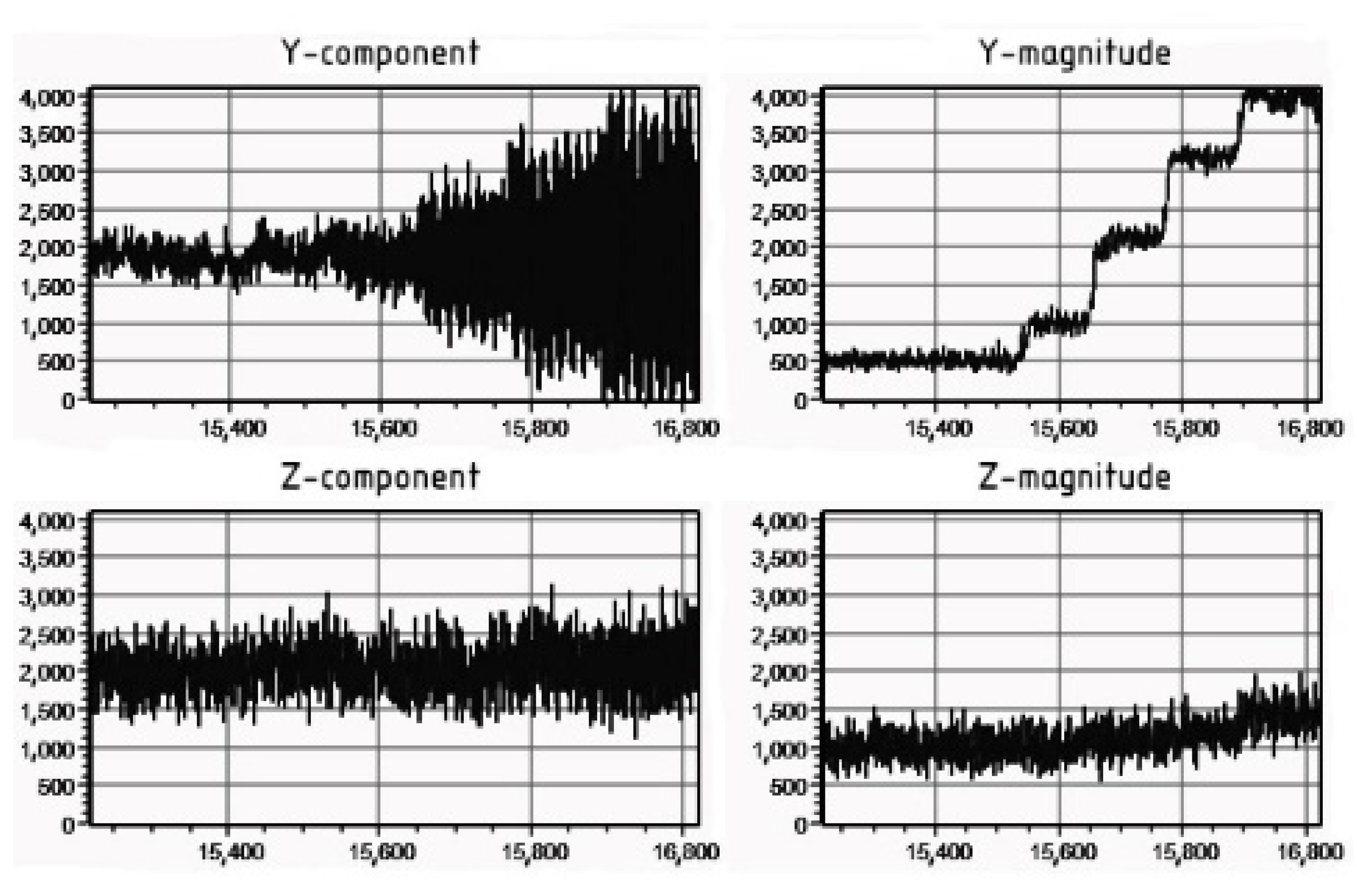
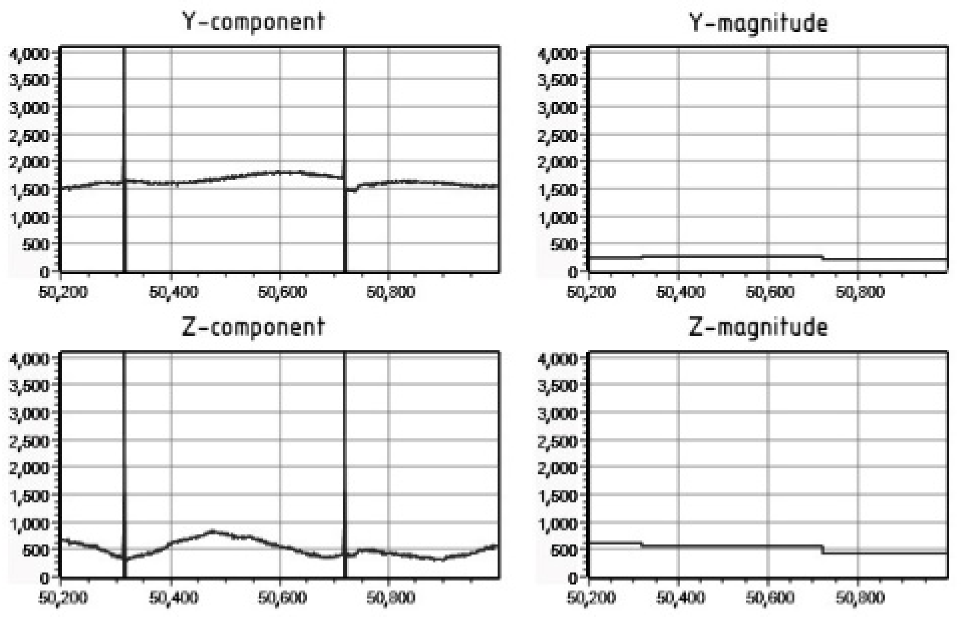
An external magnetic field with an induction value of over 1 µT introduces significant changes in the topology of the magnetic field of an energized conductor. The degree of the magnetic field topology change depends on the current value in the conductor: the smaller the current value, the stronger the influence of the external magnetic field. For example, let us consider the results of the electromagnetic field modeling in the computational domain with a distance of 3 m between the body of the microtunneling shield and the energized cable. The results of calculating the magnetic flux density along the control line are shown in
Figure 3. An external magnetic field with an induction of 10 nT does not have a significant effect on the topology of the magnetic field of an energized cable compared to the case without an external magnetic field. An external magnetic field with an induction of 1 µT with a current value of 300 A results in a significant change in the induction along the control line at a distance of over 2.7–2.8 m from the cable axis, and with a current of 50 A, significant changes occur already at a distance of 0.8–0.9 m from the cable axis. One can also note the appearance of a local minimum of the magnetic flux density value in the immediate vicinity of the tunneling shield body end (distance 2.9 m from the cable axis). The minimum value of the magnetic flux density along the control line with an external field induction of 10 µT for a current value of 50 A is achieved at a distance of 0.9 m from the conductor, and for a current of 300 A only at 2.7 m. In this situation, the value of the local minimum is a sequence higher than for the case with a magnetic field induction of 1 µT. An external field with a magnetic flux density of 1 mT results in a significant change in the topology of the energized cable electromagnetic field. Significant changes already occur at distances of 0.1–0.2 m from the axis of the energized cable and at distances of over 0.7–0.8, the value of the magnetic flux density along the control line is almost independent from the current in the cable. Thus, an increase in current from 50 A to 300 A results in a magnetic flux density growth of 4.5% at a distance of 1 m, while at an external field flux density value of 1 µT, the change was 85%.
In the absence of an external magnetic field source, the values of induction in the ferroprobe cores corresponded (considering changes in the model) to the values obtained in the paper [
4]. Considering the relative position of the energized cable and the microtunneling shield, the most significant changes in the magnetic flux density with a change in the cable current will be observed in the cores of the Y-components of ferroprobes, which was also demonstrated in [
4,
5,
6].
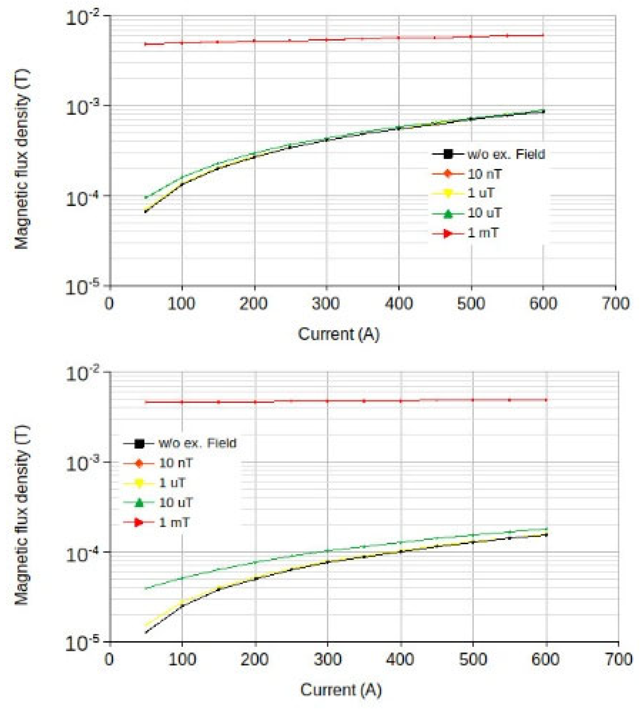
Figure 4 shows the dependencies of the values of the Y-component of the magnetic field vector in the core of ferroprobe No. 1 on the current value in the cable for various values of the external magnetic field induction.
Figure 5 shows similar dependencies for the Z-component.
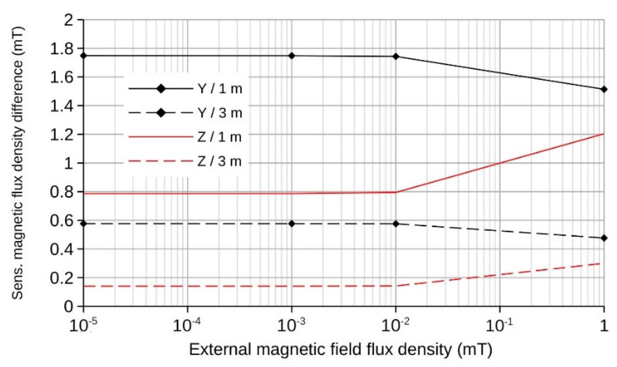
An external magnetic field with an induction of over 10 µT has a significant effect on the value of magnetic flux density in the ferroprobe cores; however, the ability of ferroprobes to detect changes in the value of magnetic flux density with a change in the current in the cable worsens insignificantly (
Figure 6). The difference between the values of the Y-component of the magnetic field vector in the ferroprobe core and the current strength in the 50 A and 600 A cables without an external field and 1 m distance between the microtunneling shield and the cable axis is 1748.9 µT. When exposed to an external field with an induction value of 1 µT, the difference decreases to 1748.3 µT, and when the magnetic flux density of the external field is 10 µT, it decreases to 1743.4 µT. Furthermore, only an external field with an induction value of 1 mT results in a decrease in the difference of the Y-component to 1514 µT. With an increase in the distance between the microtunneling shield and the cable axis to 3 m, the difference in the values of the Y-component of the magnetic field vector in the ferroprobe core between the current strength in the cable of 50 A and 600 A in the absence of an external field, decreases to 576.6 µT. An external magnetic field with an induction value of up to 10 µT does not cause a significant decrease in the difference between the values of the Y component. With an increase in the magnetic flux density value of the external field to 1 mT, the difference in the values of the Y-component decreases to 476.6 µT. The nature of the change in the difference between the values of the Z-component is similar but has a trend towards an increase in the value with an increase in the value of the external field induction.
The results show the possibility of registering the Y- and Z-components of the electromagnetic field of an energized power cable by ferroprobes in the body of a microtunneling shield at an external magnetic field induction of up to mT-sized values.


