Incorporating Human Preferences in Decision Making for Dynamic Multi-Objective Optimization in Model Predictive Control

Abstract

We present a new two-step approach for automatized a posteriori decision making in multi-objective optimization problems, i.e., selecting a solution from the Pareto front. In the first step, a knee region is determined based on the normalized Euclidean distance from a hyperplane defined by the furthest Pareto solution and the negative unit vector. The size of the knee region depends on the Pareto front’s shape and a design parameter. In the second step, preferences for all objectives formulated by the decision maker, e.g., 50–20–30 for a 3D problem, are translated into a hyperplane which is then used to choose a final solution from the knee region. This way, the decision maker’s preference can be incorporated, while its influence depends on the Pareto front’s shape and a design parameter, at the same time favorizing knee points if they exist. The proposed approach is applied in simulation for the multi-objective model predictive control (MPC) of the two-dimensional rocket car example and the energy management system of a building.

1. Introduction

Throughout the last few decades, multi-objective optimization (MOO) has attracted a lot of attention, especially from the evolutionary optimization community. With increasing computational capacities, new methods to determine (an approximation of) the Pareto front arise regularly. The selection of a solution from the Pareto front is usually left to a human decision maker (DM), which is suitable in the context of one-time optimization, e.g., in product design.

However, multi-objective optimization can be used for more than one-time optimizations. In previous works, we proposed to combine it with Model Predictive Control (MPC) [1,2], i.e., to utilize multi-objective optimization in the permanent (optimal) control of a dynamic system. The main principle is to repetitively formulate a multi-objective optimal control problem at every time step, derive an approximation of its Pareto front, and then select a single Pareto solution. This Pareto solution corresponds to a sequence of inputs (i.e., the decision variables), from which the first element is applied to the system. Then, in the next time step, the entire process is repeated.

For the real-time control of e.g., an energy management system, this means that a decision had to be made approximately every 15 min, which is too tedious for a human. For other systems with higher dynamics, this would be even worse. Thus, this process has to be automated. So far, different methods to this end exist. Unfortunately, most of them do not incorporate the preferences of a human decision maker. If they do, they usually have other drawbacks, e.g., being limited to two objectives or lacking a clear interpretation of how the preferences affect the final choice. Moreover, these methods rely significantly on the Pareto front’s extreme points. However, since also the process of determining the Pareto front is automated and the optimization problem’s objectives as well as constraints may vary over time, it is not guaranteed that the actual extreme points are found. This setting of varying objective functions and objectives over time is also called dynamic multi-objective optimization [3].

In this work, we aim to overcome these problems in dynamic multi-objective optimization. Our main contributions are that we

• Formulate a new adaptation of a well-known deterministic method to sample an approximation of the Pareto front, which is more apt for the dynamic multi-objective optimization case where objectives may correlate sometimes,
• Present a new two-step approach for the automated decision making process, which is again designed for the use in dynamic multi-objective optimization and

  ∘

  In its first step uses a definition of a knee region which depends less on accurate extreme points;

  ∘

  In its second step uses a geometric interpretation of a hyperplane representing the preferences of a decision maker formulated a priori; and

• Show in a simulation study of an energy management system that the approach leads to a proper representation of the preferences not only in the limited time horizon of the multi-objective optimization problem but also in the long-term costs.

Figure 1 illustrates the incorporation of our approach in an MPC application with multiple objectives. The rest of the paper is structured as follows. We define the MOO problem, show how it can be solved with the normal boundary intersection (NBI) method, and review the available methods for the decision making process in Section 2. The methodology of the proposed two-step decision making approach is described in Section 3. We formulate the focus point boundary intersection (FPBI) method as an alternative to the normal boundary intersection in Section 4. We discuss the consequences of incorporating multi-objective optimization in Model Predictive Control and apply the proposed methods to two examples of different complexity in Section 5 before we finish with a conclusion in Section 6.

Notation

${\mathbb{R}}_{+}^n$ denotes the n-dimensional $\mathbb{R}\ge 0$. For vectors, a subscript i as in $J_i$ denotes its i-th value. A superscript j marks the vector as a specific point from a set of points, e.g., $J^j\in \mathbb{J}$.

2. Related Work

2.1. Problem Formulation

A MOO problem can be formulated as

$$\begin{array}{}\mathrm{(1a)}& \hfill minJ(z)& =& \left(J_1(z), \dots , J_n(z)\right)\hfill \mathrm{(1b)}& \hfill s.t.& & g_j(z)\le 0, j=1,2,\dots ,m_{\mathrm{ineq}}\mathrm{(1c)}& & & h_l(z)=0, l=1,2,\dots ,m_{\mathrm{eq}},\end{array}$$

where $z\in \mathbb{Z}$ is the decision variable vector, n is the number of objectives and $m_{\mathrm{ineq}}$ and $m_{\mathrm{eq}}$ are the numbers of inequality and equality constraints, respectively. Since there typically is no single solution which minimizes all objectives $J_i$ at the same time, the concept of Pareto optimality is used. A solution $z^{*}$ is Pareto optimal if it is not dominated by any other solution, i.e., there is no solution z for which $J_i(z)\le J_i(z^{*})\forall i\in [1,n]$ and $J_k(z)<J_k(z^{*})$ for at least one $k\in [1,n]$. All Pareto optimal solutions together form the Pareto front. However, usually only a set of solutions $\mathbb{J}=\{J^1,\dots ,J^N\}$ which approximates the Pareto front can be determined. Important points apart from the Pareto front are the Utopia and the Nadir point. The Utopia point can be constructed from the Pareto front’s extreme points. An extreme point is the Pareto solution with the minimum value for its corresponding objective; i.e., the extreme point for objective i is

$$J^{\mathrm{extreme},i} = \underset{J\in \mathbb{J}}{arg\; min}{J}_i.$$

(2)

The Utopia point then consists of the single minima of all objectives

$$J^{\mathrm{utopia}} = \left(J_1^{\mathrm{extreme},1}, \dots , J_n^{\mathrm{extreme},n}\right)$$

(3)

and is thus generally not attainable. Similar, the Nadir point is the combination of all objectives’ worst values on the front, i.e.,

$$J^{\mathrm{nadir}} = \left(\underset{J\in \mathbb{J}}{sup}{J}_1, \dots , {sup}_{J\in \mathbb{J}}{J}_n\right).$$

(4)

In general, three categories of how a solution (or decision) to the MOO problem (1) can be derived exist. A priori (or explicit) methods respect the preferences or interests of the decision maker by calculating Pareto solutions on specific areas of the Pareto front. Interactive (or progressive) methods ask the decision maker for input during the optimization process itself, also to focus on specific areas. A posteriori (or implicit) methods respect the decision maker’s preferences only after the Pareto front has been approximated to select a compromise from it. Our approach presented in this paper belongs to the last group, i.e., the a posteriori methods.

In the following, we will first shortly explain how an approximation of the Pareto front can be obtained. Afterwards, we focus on the different available decision making strategies to illustrate the necessity and novelty of our proposed approach.

2.2. Determining the Pareto Front

Two different main options exist to obtain an approximation of the Pareto front for the multi-objective optimization problem (1): meta-heuristic (evolutionary strategies, genetic algorithms, etc.) or deterministic (mathematical programming) methods. Meta-heuristic methods can be considered the standard choice. Their biggest advantage is that they can be used for any optimization problem, even with black box models, as long as one can evaluate the objective function, e.g., by simulation. However, this comes at the cost of high and possibly unpredictable computation times and the uncertainty regarding whether a global (or even local) optimum has been found. This makes them less apt for the setup considered here, i.e., the repeated solving of multi-objective optimization problems for, e.g., real-time control. Therefore, we omit any further descriptions of meta-heuristic methods here and refer the interested reader to [4,5].

Approximating the Pareto front with deterministic methods means to repeatedly solve a single-objective optimization problem with different parameters. Thereby, these parameters are varied iteratively such that a different point of the Pareto front is determined each time. Such a combination of the objectives into a single scalar objective function (instead of the objective vector as in (1a)) is called scalarization. Two groups of scalarization methods are commonly used for the above purpose. The first utilizes weighted sums, possibly with exponential expressions of the objectives. The second we call—due to the lack of a better term—intersection methods, since they aim at finding the intersection of the Pareto front with some geometric entity, usually a vector.

The idea to scalarize the multi-objective optimization problem (1) by, for example, maximizing the length of a vector, dates back to the 1970s [6] and has been varied since then [7]. In general, a geometrization of the objective space is used to reformulate the optimization problem such that the actual objective function appears in the constraints only. The normal boundary intersection (NBI) was then introduced as a method of systematically varying the scalarizations to obtain a reasonable approximation of the Pareto front [8]. The procedure is as follows. First, the extreme points have to be determined. Second, a simplex connecting the extreme points is constructed, which is called the convex hull of individual minima (CHIM). Then, this simplex is sampled evenly. This can be expressed with the $n\times n$ matrix $\Phi$, whose i-th column is

$$\begin{array}{ccc}\hfill \Phi (:,i)& =\hfill & J^{\mathrm{extreme},i}-J^{\mathrm{utopia}}.\end{array}$$

(5)

The CHIM is sampled by $\Phi \beta$ with a varying $(n\times 1)$-vector $\beta$, s.t.

$$\begin{array}{ccc}\hfill {\displaystyle \sum _{i=1}^q}{\beta }_i& =\hfill & 1,{\beta }_i>0.\end{array}$$

(6)

A Pareto solution is then obtained by maximizing the length $\kappa$ of the CHIM’s normal vector $\widehat{n}$ pointing toward the Pareto front, with the constraint that the vector’s tip ends at the Pareto solution itself. For a combination $\beta$, the MOO problem (1) is then replaced by

$$\begin{array}{}\mathrm{(7a)}& & & min-\kappa \hfill \mathrm{(7b)}& \hfill s.t.& & \Phi \beta +\kappa \widehat{n}=J(z)-J^{\mathrm{utopia}}\hfill \mathrm{(7c)}& & & g_j(z)\le 0,j=1,2,\dots ,m_{\mathrm{ineq}}\hfill \mathrm{(7d)}& & & h_l(z)=0,l=1,2,\dots ,m_{\mathrm{eq}}.\hfill \end{array}$$

Note that (7) is the same if (7a) is replaced by $max\kappa$. Furthermore, the optimization problem’s solvability might be changed, since all possible nonlinearities are shifted to the constraints instead of the objective function, which is one of its disadvantages, next to its susceptibility to weakly Pareto optimal solutions. The original normal boundary intersection as described here has been modified in different ways since its introduction in 1998 [9,10,11,12]. However, since this is not the focus of this work, we omit a further description of the detailed differences.

2.3. Decision Making (Choosing a Solution)

Once an approximation of the Pareto front has been obtained, a single solution has to be chosen. To this end, various types of a posteriori methods exist. They can be categorized by whether they

• Select a final solution by themselves or only identify a subset of solutions which are then presented to the decision maker (DM);
• Aim at selecting a good compromise in general (i.e., a compromise solution) or rank the solutions in dependence of the Pareto front’s shape (i.e., try to identify a knee point);
• Do or do not incorporate preferences of a decision maker.

In the following, we give an overview of the most prevalent methods in the literature. Note that, however, different combinations of the above categories exist, such that the following order is partially arbitrary.

The most common approach is to select a final (compromise) solution using Euclidean distance-based metrics. For example, LINMAP minimizes the weighted distance to the Utopia point [13]. One could argue that the weights represent the decision maker’s preferences. However, since weighting can be problematic in general, frequently, the unweighted but normalized distance is minimized instead [1,14]. TOPSIS is an algorithm which considers both distances to the Utopia and the Nadir point [15].

Fuzzy logic is utilized in many methods for different goals but usually to select a single compromise solution, too. For example, it can be used to address uncertain objectives, constraints or decision variables [16] but also to incorporate preferences from linguistic values [17]. In [18], it is used on top of the concept of k-optimality to loosen the crisp definition of Pareto optimality. Overall, the literature on different fuzzy approaches is rich.

An alternative to fuzzy logic for decision making under uncertainties is Evidential Reasoning [19]. Multiple attributes are weighted according to their importance. For each attribute, possible grades are defined, and the likelihood of a solution’s attribute to match them are assessed, e.g., a likelihood of $0.3$ to be ’good’ and $0.6$ to be ’very good’. Then, a single overall score of the solution can be derived, and all Pareto solutions ranked accordingly.

Another concept is the use of Shannon Entropy [20]. For each objective, the solutions’ entropy is calculated, which depends on their diversity. From these, weights for every objective are derived. Then, the (normalized) solution which fits the weights best is selected.

In contrast to the compromise solutions described above, the possibly more popular aim is the selection of a knee point, which in general is a solution on the Pareto front from which a small improvement in one direction (objective) would lead to a large(r) deterioration in all others. Thus, the shape of the Pareto front is essential.

Different possibilities to define (or find) a knee point exist. Multiple approaches do so based on the point’s angle to other parts of the front, e.g., the reflex angle [21], the bend angle [22], the extended angle dominance [23] or the angle utility [23]. Utility-based methods generally define a knee by the best trade-off, i.e., the best ratio of improvements vs. deteriorations compared to all other solutions [22,24,25]. This approach is extended to multiple regions of the Pareto front in [26], i.e., the best trade-off for each region is determined. In [27], knee points are identified by mapping the Pareto front onto a hyperplane. Then, a solution is considered to be a knee point if the other solutions are densely located around it. According to [21], a point is a knee point if it is the result of the optimization of a weighted sum for multiple (different) weight combinations. In an early work, Das [28] characterizes the point with the largest distance to the convex hull of individual minima as the knee.

As an alternative to selecting a single solution (either compromise solutions or knee point), a subset or multiple subsets of the Pareto front which show knee-like behavior or other properties of interest are often determined and presented to the decision maker. Then, the decision maker has to select a final solution from this compromise manually. Note that as mentioned before, this is not applicable for the use case proposed in this paper. However, since the possibilities to do so are relevant for our proposed approach, we cover the most important methods.

If the assignment of a Pareto solution to the subset of interest is based on a metric as explained above, the subset is usually called the knee region. Examples are the trade-off-based knee region [22] or the bulge of points with the largest distance to the convex hull of individual minima [29].

If the assignment is based on the decision maker’s preference, the subset might be called region of interest. In [30], the decision maker defines a cost reference point, i.e., an arbitrary chosen $J^{\mathrm{ref}}=\left(\begin{array}{ccc}{J}_1^{\mathrm{ref}},& ...,& J_n^{\mathrm{ref}}\end{array}\right)$, either infeasible or feasible. Then, imagining a coordinate plane with $J_{\mathrm{ref}}$ at its origin, the part of the Pareto front that dominates $J_{\mathrm{ref}}$ (if feasible) or that is dominated by $J_{\mathrm{ref}}$ (if infeasible) is considered as the region of interest. Note that a drawback of this method is that it is unclear how large the region of interest will be. In [31], the decision maker defines a starting point and a preference direction. Then, the part of the Pareto front which lies within a pre-defined preference radius around the preference direction is defined as the region of interest. Again, no final solution is provided, and possible knee points are ignored.

In summary, there are many methods to choose a solution to the MOO problem (1) once an approximation of the Pareto front has been determined. However, there is no method which (1) selects a single solution (instead of a subset of solutions), (2) thereby prefers knee points (if they exist) and (3) at the same time includes preferences of a decision maker in a comprehensible way. We try to fill this gap with the approach explained next.

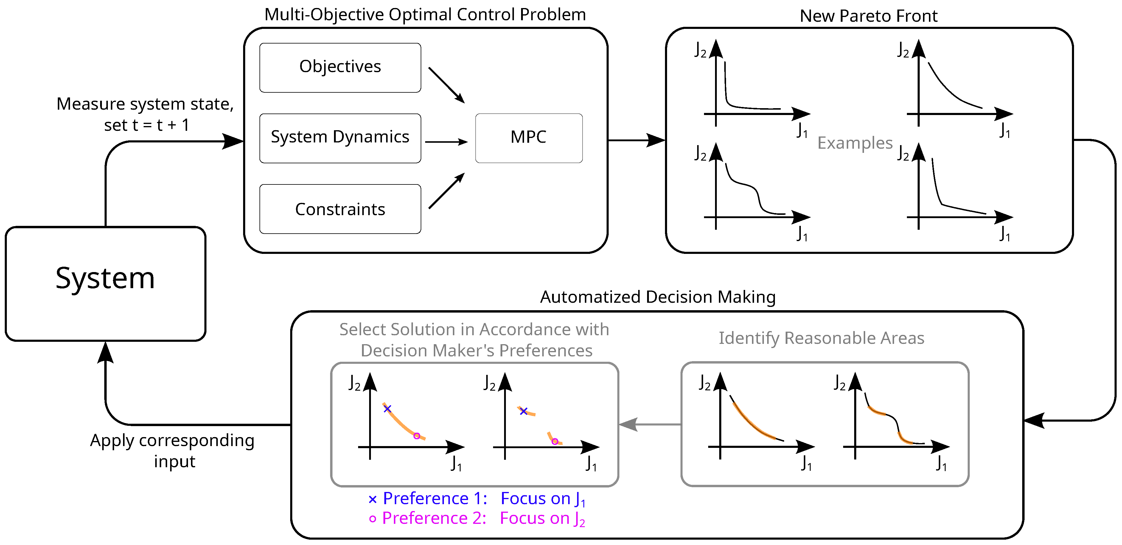
3. Proposed Automatized Decision Making Approach

We assume to have an approximation $\mathbb{J}$ of the Pareto front. Then, the approach consists of two parts. First, the knee region is determined. Second, a solution is finally chosen in dependence of the decision maker’s preferences.

All further calculations are done in the normalized space $\tilde{\mathbb{J}}$. Namely, all objective values $J^i\in \mathbb{J}$ are normalized as

$${\tilde{J}}_{\ell }^i = \frac{J_{\ell }^i-J_{\ell }^{\mathrm{Utopia}}}{J_{\ell }^{\mathrm{Nadir}}-J_{\ell }^{\mathrm{Utopia}}}.$$

(8)

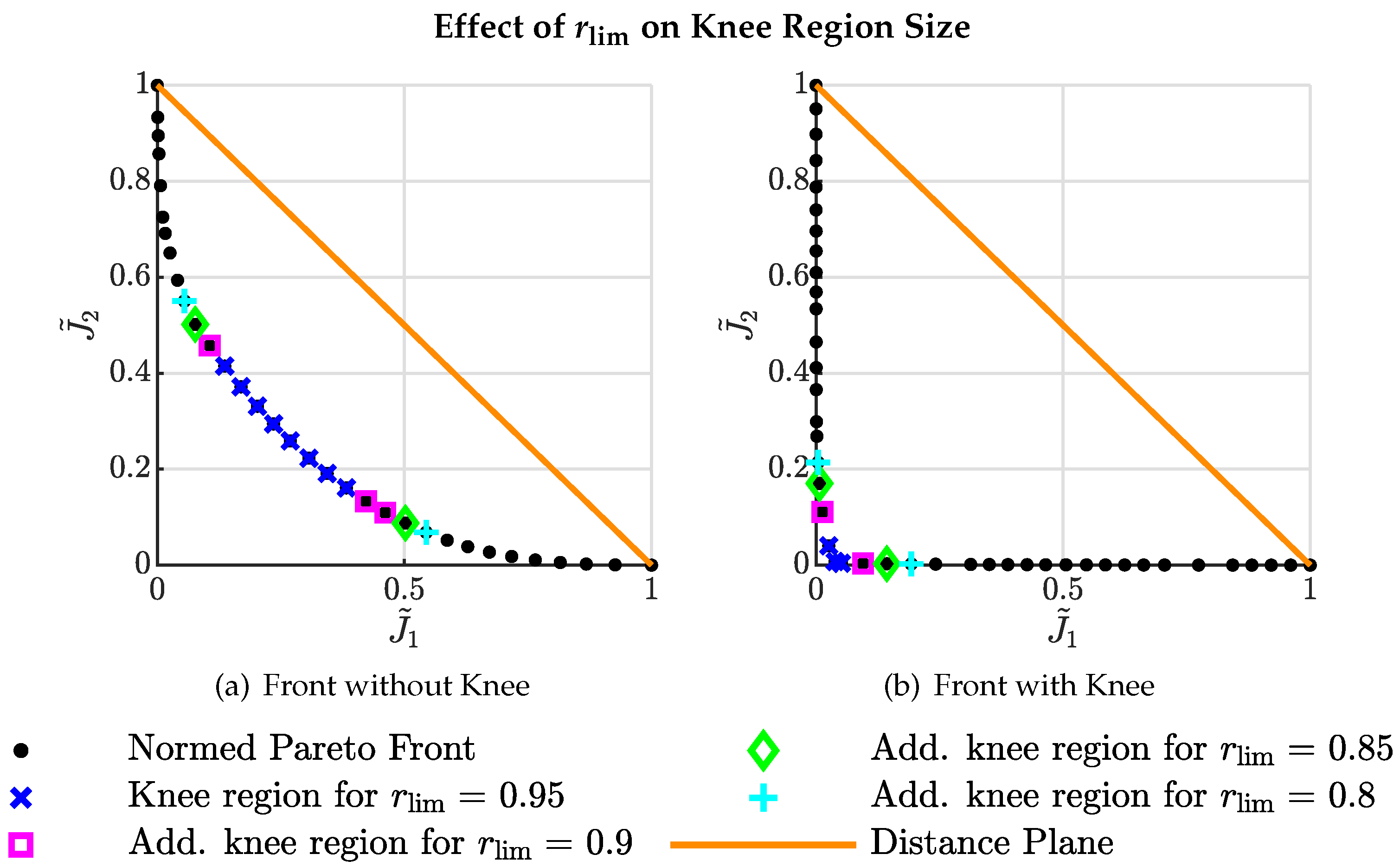
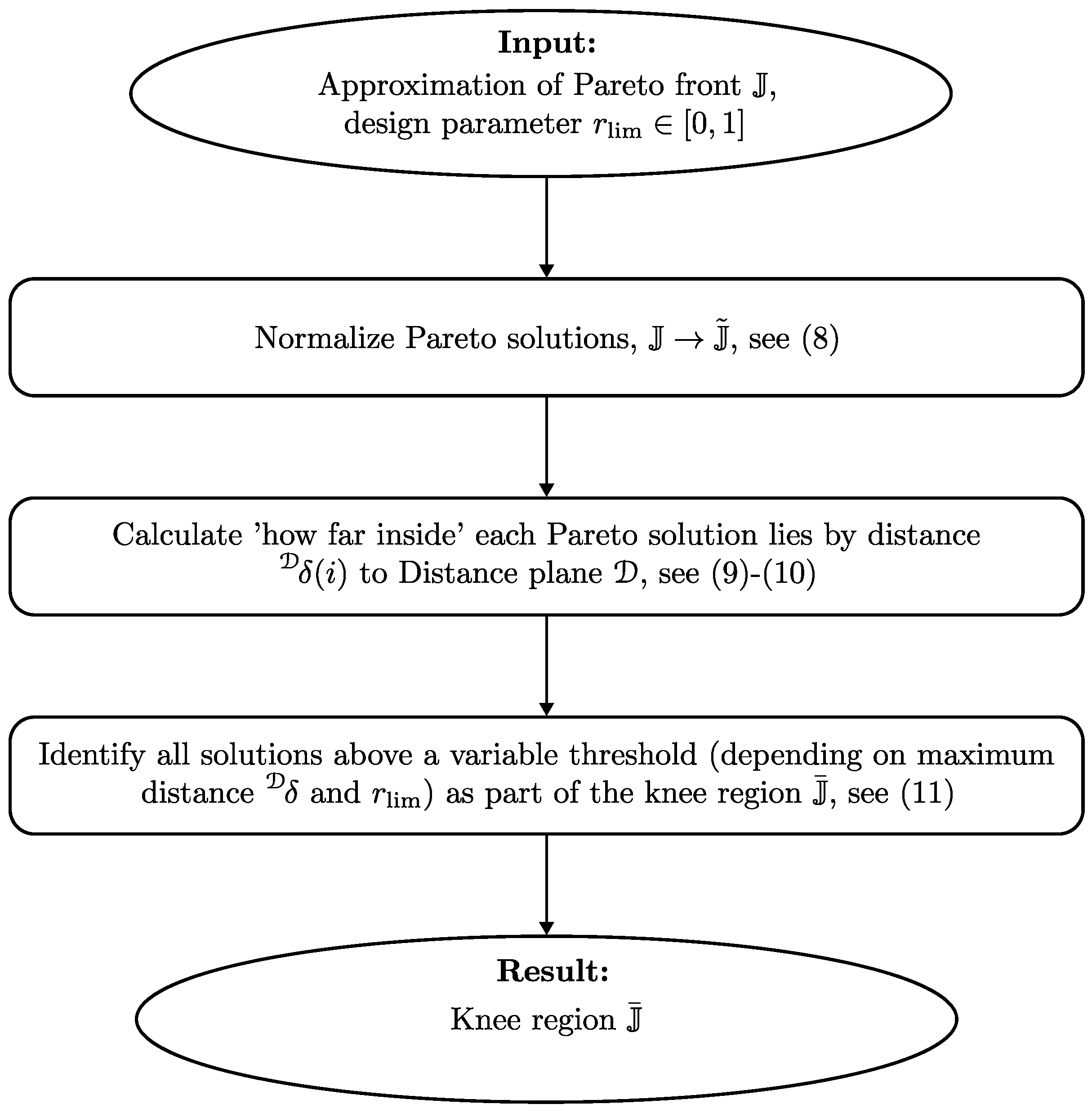
3.1. Knee Region Determination

For the definition of our knee region, we use a metric similar to [28]; i.e., for each Pareto solution, we calculate its Euclidean distance to a geometric object at the edge of the Pareto front. However, the individual minima (also called extreme points) are often hard to find [24,32]. Thus, instead of maximizing the distance from the convex hull of the extreme points, we use a hyperplane

$$\mathcal{D} : \{x|-e^{⊺}(x-{\tilde{J}}^q)=0,q=\underset{i}{arg\; max}||{\tilde{J}}^i|{|}_2\}$$

(9)

which we refer to as the distance plane in the following. Note that ${\tilde{J}}^q\in \tilde{\mathbb{J}}$ is the point of the (normalized) Pareto front with the largest Euclidean distance to the normalized Utopia point ${\tilde{J}}^{\mathrm{utopia}}=\left(\begin{array}{c}0\dots 0\end{array}\right)$ and that we use the negative unit vector $-e=-{\mathbf{1}}_{n\times 1}$ as the distance plane’s normal vector to avoid sensitivity to possibly unreliable extreme points. Then, the distance of every solution ${\tilde{J}}^i\in \tilde{\mathbb{J}}$ to $\mathcal{D}$ is calculated as

$${}^{\mathcal{D}}\delta (i) = \frac{1}{\sqrt{n}}(-e^{⊺})({\tilde{J}}^i-{\tilde{J}}^q).$$

(10)

Finally, similar to [29,33], we define the knee region $\overline{\mathbb{J}}\subseteq \tilde{\mathbb{J}}$ as

$$\overline{\mathbb{J}} = \{{\tilde{J}}^i|{}^{\mathcal{D}}\delta (i)\ge r_{\lim }·{}^{\mathcal{D}}\delta (z),z=\underset{i}{arg\; max}{}^{\mathcal{D}}\delta (i)\},$$

(11)

where $r_{\lim }\in [0,1]$ is a design parameter with which the influence of the decision maker’s preferences can be adjusted. Furthermore, (11) can be understood as a bulge of the Pareto front in the direction of the Utopia point, whose size depends on the Pareto front’s shape, as illustrated in Figure 2. Note that in contrast to the commentary in [29], while the bulge is hard to comprehend in more than three dimensions, this is not necessary for our approach, since the final decision making is automatized, too. Figure 3 summarizes the procedure.

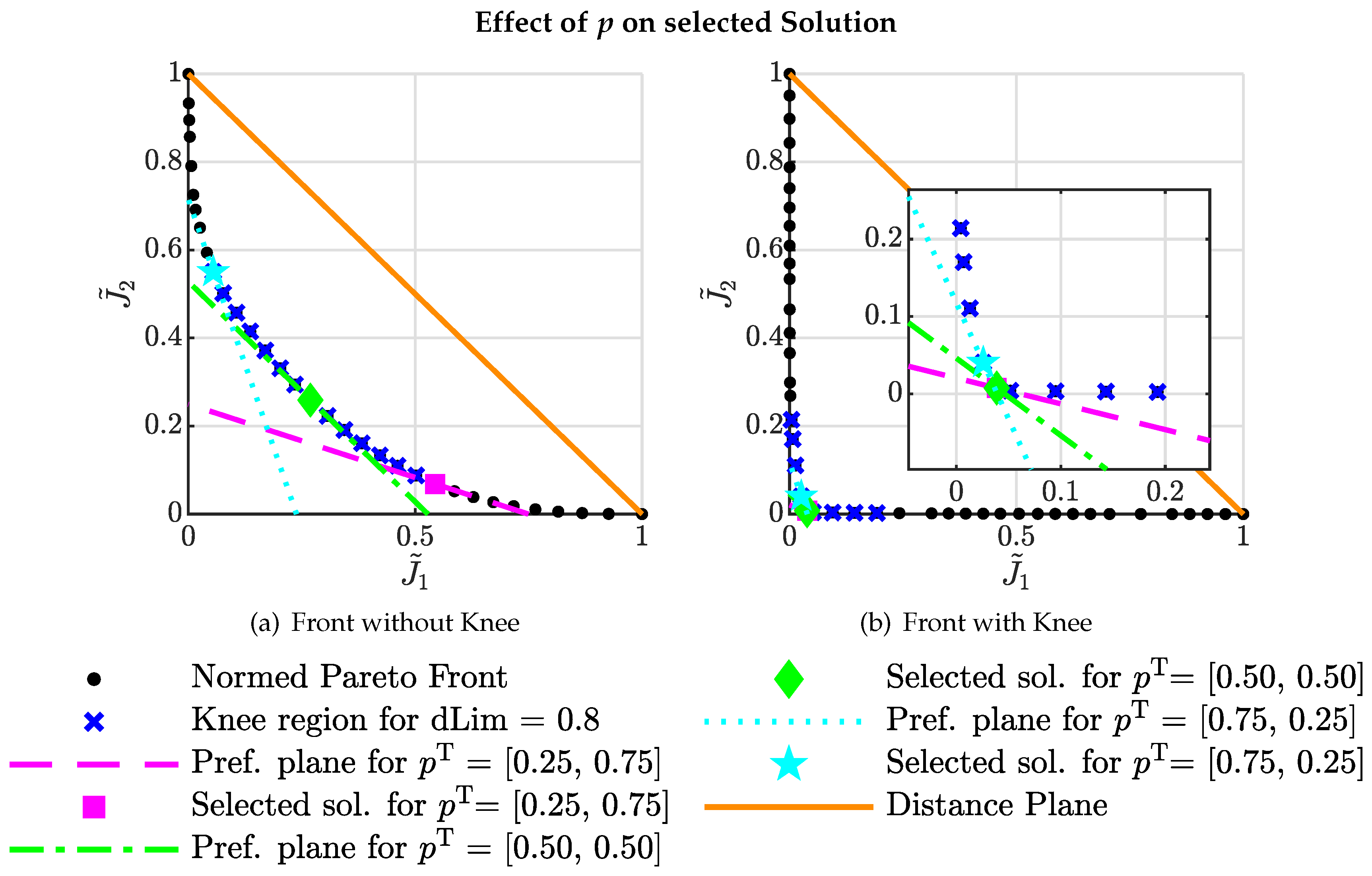
3.2. Choosing a Solution

After the knee region $\overline{\mathbb{J}}$ has been determined, one of its solutions has to be chosen. First, the preferences of the decision maker are formulated as the preference vector $p\in {\mathbb{R}}_{+}^n$ for all n objectives. Since we work in the normalized space, the objectives’ possibly different magnitudes can be ignored. Then, p can be interpreted as the normal vector of a hyperplane

$$q({\tilde{J}}^{\mathrm{b}}) : \{x|p^{⊺}(x-{\tilde{J}}^{\mathrm{b}})=0\}$$

(12)

where ${\tilde{J}}^{\mathrm{b}}\in \overline{\mathbb{J}}$ is the hyperplane’s base point. In the following, we will refer to $\mathcal{P}$ as the preference plane.

As base point ${\tilde{J}}^{\mathrm{b}}$, we choose the knee region’s solution to which the preference plane is ’tangential’, i.e., the ${\tilde{J}}^{\mathrm{b}}={\tilde{J}}^i\in \overline{\mathbb{J}}$ that builds a halfspace with the preference plane which lies below all other solutions, such that

$$p^{⊺}({\tilde{J}}^j-{\tilde{J}}^{\mathrm{b}})\ge 0\forall {\tilde{J}}^j\in \overline{\mathbb{J}}.$$

(13)

In 2D, this halfspace is the area below a line, and the line passes through ${\tilde{J}}^{\mathrm{b}}$ and is orthogonal to p. In the unlikely event that multiple solutions on the knee region fulfill (13), any of them can be selected. Figure 4 illustrates different preference planes and the resulting selections for a 2D front; Figure 5 summarizes the selection procedure.

3.3. Influence of Imperfect Extreme Points

As stated at the beginning of this section, we assume to have an approximation $\mathbb{J}$ of the Pareto front, which includes the extreme points for all objectives. These may influence the final decision significantly due to the normalization scheme (8). However, the determination of the (real) extreme points is often challenging. Thus, in the following, we analyze the effect of imperfect (i.e., underestimated) extreme points for an artificial Pareto front with significantly different magnitudes of two objectives, i.e.,

$$J_2 = \frac{1}{log(J_1+1)}.$$

(14)

Since ${lim}_{J_1\to 0}{J}_2=\infty$, we restrict $J_1$ to $J_1\in [0.001,1]$, which leads to $J_2\in [1.44,1000.50]$. The critical extreme point is the one for $J_2$. Thus, we compare the calculated knee regions and selected solutions for various underestimated $J^{\mathrm{extreme},2}$. Figure 6 shows the results for different settings, which illustrate the dependence of the selected solution on the assumed extreme points. However, this is not a specific weakness of the proposed approach here but a problem that all decision making approaches presented in Section 2.3 share, since they either use a normalization scheme similar to (8), and/or use the extreme points in their utility calculations, e.g., for the angle of a single solution to the extreme points (bend angle).

If for a specific problem, the accurate determination of the extreme points is problematic and the objectives’ magnitudes differ significantly, it might be beneficial to normalize the Pareto front with fixed values instead of the dynamic normalization in dependence of the extreme points. Values for such a fixed normalization scheme can be obtained from long-term simulations, as is explained in [2].

3.4. Discussion of the Preference for Knee Points

As stated in Section 2.3, Ref. [21] defines the knee point of a 2D MOO problem as the point which is the solution for the most ${\lambda }_i$ in the weighted sum

$$\underset{x}{min}{\lambda }_i·J_1(x)+(1-{\lambda }_i)·J_2(x)$$

(15)

where ${\lambda }_i$ is chosen from a large but finite set $\subseteq [0,1]$. However, as illustrated in [22] (Figure 1) and explained in [34], the minimization of (15) can be interpreted as shifting a plane with angle $\alpha ({\lambda }_i)$ to the origin until it is tangential to the Pareto front. Furthermore, this interpretation is also applicable with n-dimensional hyperplanes, see e.g., [35]. Thus, our approach of constructing a hyperplane a posteriori and choosing the solution at which it is tangential to the Pareto front inherently prefers knee points, since multiple preferences p (and thus preference planes) will satisfy (13) for the same $J^i$ if it is a knee point (as the small illustration in Figure 4b suggests). However, note that this does not allow the conclusion that our approach could be replaced by solving a weighted sum with the according weights instead. First, the reduction of possible decisions to a knee region prevents too extreme (and thus uninteresting) points to be selected, independently of the formulated preferences. Second, our approach allows us to use an approximation of the Pareto front which can be derived from any method, not just from the minimization of a weighted sum.

4. Focus Point Boundary Intersection Method

In the following, we present an adaption of the normal boundary intersection method. It is more apt for the proposed setup of multi-objective optimization in combination with Model Predictive Control. Namely, due to varying conditions over time, objectives may correlate sometimes. This would lead to a degenerate Pareto front [36]. Even if they do not correlate perfectly, some extreme points may end up very close to each other. If this is the case for two out of three objectives, the resulting simplex (i.e., the convex hull of individual minima (CHIM)) is a very narrow triangle. Then, in combination with the search direction being strictly orthogonal to the simplex, this might lead to almost no real Pareto solutions being found.

Thus, we propose the focus point boundary intersection (FPBI) method. In contrast to the normal boundary intersection, it (1) constructs a hyperplane which depends less on the extreme points and (2) enables the decision maker to define a search direction to increase the probability of finding solutions in the area of interest. If no specific goal is available, we use the Utopia point. Figure 7 gives an overview of the procedure.

The procedure of the proposed focus point boundary intersection method is as follows. We assume that the Pareto front’s extreme points $\{J^{\mathrm{extreme},1},\dots ,J^{\mathrm{extreme},n}\}$ are known. Moreover, all further calculations are again done after the normalization $J\to \tilde{J}$ of the solutions as in (8), such that each objective lies within $[0,1]$ in the normalized space $\tilde{\mathbb{J}}$.

First, we determine the extreme points $(a,b)$ between which the distance is the longest,

$$(a,b)=\underset{(i,j)\in [1,\dots ,n]}{arg\; max}{∥{\tilde{J}}^{\mathrm{extreme},i}-{\tilde{J}}^{\mathrm{extreme},j}∥}_2.$$

(16)

With $(a,b)$ known, we determine the center point between them,

$$\begin{array}{ccc}\hfill {\tilde{J}}^{\mathrm{center}}& =\hfill & \frac{1}{2}({\tilde{J}}^{\mathrm{extreme},a}+{\tilde{J}}^{\mathrm{extreme},b}).\end{array}$$

(17)

The search direction is then defined from ${\tilde{J}}^{\mathrm{center}}$ to the focus point,

$$\begin{array}{ccc}\hfill n^{\mathrm{s}}& =\hfill & {\tilde{J}}^{\mathrm{focus}}-{\tilde{J}}^{\mathrm{center}}.\end{array}$$

(18)

If no specific focus point is given, ${\tilde{J}}^{\mathrm{focus}}={\tilde{J}}^{\mathrm{utopia}}=\left(\begin{array}{ccc}0,& \dots ,& 0\end{array}\right)$ is used, which usually gives good results.

The main idea is to use a hyperplane between the farthest extreme points $(a,b)$, sample it equidistantly in every direction, and to then solve an optimization problem similar as in the normal boundary intersection method, i.e., maximizing the length of a vector with the direction $n^{\mathrm{s}}$ from the hyperplane to the Pareto front. ${\tilde{J}}^{\mathrm{center}}$ is used as the base vector of the hyperplane. Thus, we further need $n-1$ (orthonormal) direction vectors to describe it. For $n=2$ objectives, the connection between the two extreme points already constitutes the hyperplane and

$$\begin{array}{ccc}\hfill d^1& =\hfill & \frac{{\tilde{J}}^{\mathrm{extreme},b}-{\tilde{J}}^{\mathrm{extreme},a}}{{∥{\tilde{J}}^{\mathrm{extreme},b}-{\tilde{J}}^{\mathrm{extreme},a}∥}_2}\end{array}$$

(19)

is its only direction vector. For $n=3$ objectives, the necessary second direction vector can directly be determined as the cross product of the search direction and the first direction vector,

$$\begin{array}{ccc}\hfill d^2& =\hfill & \frac{n^{\mathrm{s}}\times d^1}{{∥n^{\mathrm{s}}\times d^1∥}_2}(\mathrm{for}n=3\mathrm{only}!).\end{array}$$

(20)

For $n\ge 4$ objectives, we have additional degrees of freedom. For ease of representation, assume that $a=1,b=2$. This is no limitation, but it can be achieved by simple (temporary) re-ordering. Then, we first construct $n-2$ auxiliary direction vectors

$$\begin{array}{ccc}\hfill {\widehat{d}}^{\ell }& =\hfill & {\tilde{J}}^{\mathrm{extreme},\ell +1}-{\tilde{J}}^{\mathrm{center}}\forall \ell \in [2,\dots ,n-1].\end{array}$$

(21)

Note that we use the extreme points, since we can assume that the resulting vectors are linearly independent.

The direction vectors are then determined in increasing order by subsequently calculating the cross product of the search direction vector $n^{\mathrm{s}}$, the already known direction vectors $d^i$ and the auxiliary direction vectors ${\widehat{d}}^j$ for all other directions. To increase readability, we borrow the ⋀ symbol for the cross product of multiple vectors in the following, with which the ℓ-th direction vector is determined by

$$\begin{array}{cc}\hfill d^{\ell }& =\frac{n^{\mathrm{s}}\times {\bigwedge }_{i=1}^{\ell -1}{d}^i\times {\bigwedge }_{j=\ell +1}^{n-1}{\widehat{d}}^j}{{∥n^{\mathrm{s}}\times {\bigwedge }_{i=1}^{\ell -1}{d}^i\times {\bigwedge }_{j=\ell +1}^{n-1}{\widehat{d}}^j∥}_2}\hfill \\ & \forall j\in [2,\dots ,n-1].\hfill \end{array}$$

(22)

The generalized cross product of $n-1$ vectors can be calculated as the determinant of an extended matrix, i.e.,

$$\begin{array}{ccc}\hfill {\displaystyle \underset{i-1}{\overset{n-1}{\bigwedge }}}{v}^i& =\hfill & det\left(\begin{array}{ccccc}{\overrightarrow{e}}^1& v_1^1& v_1^2& \dots & v_1^{n-1}\\ {\overrightarrow{e}}^2& v_2^1& v_1^2& \dots & v_2^{n-1}\\ ⋮& ⋮& ⋮& \ddots & ⋮\\ {\overrightarrow{e}}^n& v_n^1& v_n^2& \dots & v_n^{n-1}\end{array}\right).\end{array}$$

(23)

Note that we exceptionally use the vector symbol ${\overrightarrow{e}}^i$ here to emphasize that these are the unit vectors, e.g., ${\overrightarrow{e}}^1={\left(\begin{array}{cccc}1,& 0,& \cdots ,& 0\end{array}\right)}^{⊺}$, and not scalar values. Equation (23) can be solved by using the Laplace expansion along the first column. In doing so, the purpose of the unit vectors becomes clear, too: they transform the minors into a vector again.

With the hyperplane defined by ${\tilde{J}}^{\mathrm{center}}$, $n^{\mathrm{s}}$ and the direction vectors, we need to sample it to determine starting points for the optimization problem. Hereby, the user can control the resolution by defining a number $r_{\mathrm{F}}$ of steps along each direction. Thus, the total number of optimization problems is $r_{\mathrm{F}}^{n-1}$. We define a $1\times r_{\mathrm{F}}$ step size vector $\gamma$ by

$$\begin{array}{}\mathrm{(24)}& \Delta s=\frac{{∥{\tilde{J}}^{\mathrm{extreme},b}-{\tilde{J}}^{\mathrm{extreme},a}∥}_2}{r_{\mathrm{F}}},\mathrm{(25)}& \gamma =\left(\begin{array}{ccc}1·\Delta s,& \cdots ,& r_{\mathrm{F}}·\Delta s\end{array}\right)-\frac{r_{\mathrm{F}}}{2}\Delta s.\end{array}$$

Let $s_i\in [1,\dots ,r_{\mathrm{F}}]$ for $i=1,\dots n-1$ be the sample indices along the $n-1$ direction vectors. For a combination $(s_1,s_2,\dots ,s_{n-1})$, the $(n\times 1)$-dimensional starting vector in the optimization problem is then given by

$$\begin{array}{ccc}\hfill \Theta (s_1,s_2,\dots ,s_{n-1})& =\hfill & {\tilde{J}}^{\mathrm{center}}+{\displaystyle \sum _{i=1}^{n-1}}\gamma (s_i)·d^i.\end{array}$$

(26)

The corresponding optimization problem is described by

$$\begin{array}{}\mathrm{(27a)}& & min-\kappa \hfill \mathrm{(27b)}& \hfill s.t.& & \Theta (s_1,s_2,\dots ,s_{n-1})+\kappa n^{\mathrm{s}}\ge \tilde{J}(z)\hfill \mathrm{(27c)}& & g_j(z)\le 0,j=1,2,\dots ,m_{\mathrm{ineq}}\hfill \mathrm{(27d)}& & h_l(z)=0,l=1,2,\dots ,m_{\mathrm{eq}},\hfill \end{array}$$

Note that we use ≥instead of = in (27b) since this led to faster convergence in practice.

5. Exemplary Case Studies

In this section, we apply the proposed decision making approach to two exemplary systems in simulation, i.e., the rocket car example and the energy management system of a building, and compare it to a simpler baseline approach. Both systems are controlled using Model Predictive Control. Before that, we comment on the combination with Model Predictive Control in general.

5.1. Remarks on the Consequences of the Application within MPC

The proposed decision making algorithm is well suited to combine multi-objective optimization with MPC. However, as with at least most multi-objective MPC schemes, theoretical properties such as stability or feasibility become hard to prove. Some works do so for a specific MOO setting.

For example, in [37], a general MOO MPC scheme for nonlinear systems is proposed. They consider a finite number of objectives and show that, given some mild assumptions in addition to the usual, the $max()$ of all objectives as the cost function can be used as a Lyapunov function to guarantee stability. In [38], a weighted sum is used. However, the weights are updated in every time step, thus choosing different Pareto solutions. It is shown that under some conditions on the objectives, e.g., joint convexity, closed-loop stability can be guaranteed. However, for the updating of the weights, a linear programming problem which is not jointly convex in general has to be solved in every time step. An economic MPC scheme with a compromise solution is formulated in [39]. Namely, the authors directly minimize the (unweighted) distance to the Utopia point. However, they only consider steady-state control and show that if the objectives satisfy a Lipschitz continuity property and strong duality, stability can be guaranteed.

To employ more sophisticated (and possibly interactive) MOO schemes such as the one proposed here in combination with MPC, we suggest to indirectly ensure stability for systems such as the one presented in Section 5.4 differently. First, the proposed algorithm should be used only for systems with an inherently stable system dynamic. For example, for a discrete linear system

$$\begin{array}{ccc}\hfill x(k+1)& =\hfill & Ax(k)+Bu(k)\end{array}$$

(28)

with the system matrix A, states $x(k)$, input matrix B and inputs $u(k)$, the autonomous subsystem $x(k+1)=Ax(k)$ should be Lyapunov stable. Second, the constraints $x\in \mathbb{X}$, $u\in \mathbb{U}$ should be chosen such that every feasible state is acceptable and that for every $x(k)\in \mathbb{X}$, a feasible solution exists such that $x(k+1),\dots ,x(N_{\mathrm{p}})\in \mathbb{X}$ and $u(k),\dots ,u(N_{\mathrm{pred}}-1)\in \mathbb{U}$. If so, the optimal control problem is always feasible independently from the chosen solution before.

5.2. Comparison Approaches

To compare the effectiveness of our proposed approach in the following examples, we present a simpler strategy as a baseline. Assume $n=3$ objectives and $p^{⊺}=[20\%,70\%,10\%]$. The preferences determine the order in which the objectives are considered in the following. For the above example, all Pareto solutions would be ranked by $J_2$ first. Then, the worst $70\%$ (in terms of $J_2$) are removed from the set of possible solutions. Next, the remaining solutions are ranked by $J_1$, from which the worst $20\%$ (in terms of $J_1$) are then removed. Finally, the remaining solutions are ranked by $J_3$ and the solution which is better than the worst $10\%$ (in terms of $J_3$) is selected.

In the simulation results presented in Section 5.3.3, Section 5.4.3 and Section 5.4.4, we also optionally combine this simple approach with the limitation to a knee region as proposed in Section 3.1. If so, the knee region $\overline{\mathbb{J}}$ is determined first as usual, and then, we select a solution from $\overline{\mathbb{J}}$ by the rules described above (instead of using the preference plane).

Note that the preferences have to be normalized first, such that ${\sum }_{i=1}^q{p}_i=100\%$. If only $n=2$ objectives are considered, the solution which splits the set in terms of the preferences can be selected directly.

5.3. Example 1: Rocket Car

As a toy example, we first apply the proposed approach to the so-called rocket car, which is controlled using multi-objective Model Predictive Control. In the following, we describe the system dynamics and the resulting optimization problem and compare the simulation results of our proposed decision making approach to the simpler baseline approaches presented above.

5.3.1. System Description

We consider the rocket car in two dimensions. Thus, it consists of two separated double integrators. Its coordinates are $\left(\begin{array}{cc}{z}_1,& z_2\end{array}\right)$, and the corresponding velocities are $\left(\begin{array}{cc}{v}_{z_1},& v_{z_2}\end{array}\right)$. Together, they form the state vector $x={\left(\begin{array}{cccc}{z}_1,& z_2,& v_{z_1},& v_{z_2}\end{array}\right)}^{⊺}$. It has two inputs, which are the acceleration in both directions, $u={\left(\begin{array}{cc}{a}_{z_1},& a_{z_2}\end{array}\right)}^{⊺}$. The dynamics are described by the time-continuous linear state space system

$$\begin{array}{}\hfill \dot{x}\left(t\right)=\left(\begin{array}{cccc}0& 1& 0& 0\\ 0& 0& 0& 0\\ 0& 0& 0& 1\\ 0& 0& 0& 0\end{array}\right)x\left(t\right)+\left(\begin{array}{cc}0& 0\\ 1& 0\\ 0& 0\\ 0& 1\end{array}\right)u\left(t\right).\end{array}$$

(29)

The discretization with the sampling time $T_{\mathrm{s}}$ leads to the discrete linear state space system

$$\begin{array}{}\hfill x(k+1)=\left(\begin{array}{cccc}1& T_s& 0& 0\\ 0& 1& 0& 0\\ 0& 0& 1& T_s\\ 0& 0& 0& 1\end{array}\right)x\left(k\right)+\left(\begin{array}{cc}0.5T_s^2& 0\\ T_s& 0\\ 0& 0.5T_s^2\\ 0& T_s\end{array}\right)u\left(k\right).\end{array}$$

(30)

The discrete system (30) shall be driven into a set point $\left(\begin{array}{cc}{z}_{1,\mathrm{goal}},& z_{2,\mathrm{goal}}\end{array}\right)=\left(\begin{array}{cc}10,& 5\end{array}\right)$ using Model Predictive Control. As the prediction horizon, we choose $N_{\mathrm{pred}}=20$ steps and $T_{\mathrm{s}}=0.5\mathrm{s}$. In the following, we denote the global time step by k and time steps within the prediction horizon by i. We optimize two competing objectives, i.e., first the deviation of the current position from the set point

$$\begin{array}{ccc}\hfill J_{\mathrm{pos}}(k)& =\hfill & {\displaystyle \sum _{i=k}^{k+N_{\mathrm{p}}}}{(z_1(i)-z_{1,\mathrm{goal}})}^2+{(z_2(i)-z_{2,\mathrm{goal}})}^2,\end{array}$$

(31)

and the energetic expense

$$\begin{array}{ccc}\hfill J_{\mathrm{energy}}(k)& =\hfill & {\displaystyle \sum _{i=k}^{k+N_{\mathrm{p}}-1}}{a}_{z_1}{(k)}^2+a_{z_2}{(k)}^2.\end{array}$$

(32)

We force the system to be in a box of side-length 0.2 around $\left(\begin{array}{cc}{z}_{1,\mathrm{goal}},& z_{2,\mathrm{goal}}\end{array}\right)$ at the end of the prediction horizon by the constraints

$$\begin{array}{}\mathrm{(33)}& -0.1\le & z_1|i=k+N_{\mathrm{pred}}|-z_{1,\mathrm{goal}}\hfill & \le & 0.1,\mathrm{(34)}& -0.1\le & z_2|i=k+N_{\mathrm{pred}}|-z_{2,\mathrm{goal}}\hfill & \le & 0.1,.\end{array}$$

Additionally, both the velocities and the accelerations are limited, i.e.,

$$\begin{array}{}\mathrm{(35)}& -4\le & v_{z_1}(k)\hfill & \le & 4,\mathrm{(36)}& -4\le & v_{z_2}(k)\hfill & \le & 4,\mathrm{(37)}& -1\le & a_{z_1}(k)\hfill & \le & 1,\mathrm{(38)}& -1\le & a_{z_2}(k)\hfill & \le & 1.\end{array}$$

The multi-objective optimal control problem is then described by

$$\begin{array}{c}min\left(J_{\mathrm{pos}}, J_{\mathrm{energy}}\right)\hfill \\ s.t.(30),\hfill \\ (33)–(38).\hfill \end{array}$$

(39)

5.3.2. Implementation

Both system dynamics and Pareto optimization, i.e., the determination of the Pareto fronts and the automatized selection as described in Section 3, have been implemented with the Matlab MPC framework PARODIS [40]. The approximation of a single Pareto front with the focus point boundary intersection method from Section 4, resulting in 19 Pareto optimal solutions at each time step, takes ≈$0.8\mathrm{s}$ on a single core of an Intel i7-8550U CPU with $1.80\mathrm{GHz}$. An entire simulation with 40 time steps takes ≈$32\mathrm{s}$.

Note that for all results presented in the following, the minimum possible costs for each objective have been subtracted. Namely, we run the simulations with each objective separately to obtain the lowest values which cannot be avoided, which are $\left(\begin{array}{cc}{J}_{\mathrm{pos}}^{\min },& J_{\mathrm{energy}}^{\min }\end{array}\right)=\left(\begin{array}{cc}632.29,& 0.0364\end{array}\right)$. This way, the effect of the preferences can be interpreted appropriately.

5.3.3. Simulation Results

We vary the preference $p_{\mathrm{pos}}$ on $J_{\mathrm{pos}}$ from 0 to 100 and the preference on $J_{\mathrm{energy}}$ reversed accordingly, such that $p_{\mathrm{pos}}+p_{\mathrm{energy}}=100$. The simulation results are shown in Figure 8.

Figure 8a,b show the resulting costs for the simple baseline approach described in Section 5.2. The position costs are extremely high for $p_{\mathrm{pos}}\le 10$ with 1247, but they decrease with increasing $p_{\mathrm{pos}}$. However, the energy costs show an unexpected increase for $p_{\mathrm{pos}}=60$, i.e., they are higher than for $p_{\mathrm{pos}}=60,p_{\mathrm{energy}}=40$ than for $p_{\mathrm{pos}}=70,p_{\mathrm{energy}}=30$, which is unwanted.

If the simple baseline approach is combined with the prior limitation to the knee region as in Figure 8c,d, the extreme solutions for the position costs are limited to 230. The unwanted bump in the energy costs for $p_{\mathrm{pos}}=60$ disappears, too, i.e., the long-term results show a better representation of the preferences. However, the transitions between the preference settings are still unsmooth. For example, the results for $p_{\mathrm{pos}}=0,10,20$ are all the same, and the differences in $J_{\mathrm{pos}}$ when increasing $p_{\mathrm{pos}}$ from $20\to 30\to 40$ are high, low and again high.

The proposed decision making approach in Figure 8e,f has a more predictable and smooth behavior. The effect of the limitation to the knee region is still observable, since the results for the extreme preference settings $p_{\mathrm{pos}}=0,10,20$ are close. However, when $p_{\mathrm{pos}}$ is further increased, the quadratic nature of $J_{\mathrm{pos}}$ is observable. The energy costs $J_{\mathrm{energy}}$ are also increased smoothly with every increase in $p_{\mathrm{pos}}$. Concluding, with our proposed approach, the preferences are represented in the long-term costs as the most predictable.

5.4. Example 2: Building Energy Management System

As a more sophisticated example, the energy management system of an office building is controlled using multi-objective MPC. Note that the energy management problem for buildings or microgrids has been a popular application for multi-objective optimization both in the design [41] and for the operation [42]. This is due to both the necessity of respecting multiple criteria as well as the relatively high step sizes, which make the use of computational expensive optimization methods possible.

Figure 8. Position and energy costs for the rocket car example with different preferences $p_{\mathrm{pos}}$ and $p_{\mathrm{energy}}$ for (a,b) the simple baseline approach, (c,d) the simple baseline approach but with limitation to the knee region, and (e,f) the proposed preference-based decision making approach, with $r_{\lim }=0.85$ for the latter two cases. Results from using the closest to Utopia point (CUP) metric are plotted for comparison.

Figure 8. Position and energy costs for the rocket car example with different preferences $p_{\mathrm{pos}}$ and $p_{\mathrm{energy}}$ for (a,b) the simple baseline approach, (c,d) the simple baseline approach but with limitation to the knee region, and (e,f) the proposed preference-based decision making approach, with $r_{\lim }=0.85$ for the latter two cases. Results from using the closest to Utopia point (CUP) metric are plotted for comparison.

5.4.1. System Description

For the considered office building, the system states are the building temperature ${\vartheta }_{\mathrm{b}}$ and the stored energy E of a stationary battery. The controllable inputs are an air conditioning unit ${\dot{Q}}_{\mathrm{cool}}$, a gas radiator ${\dot{Q}}_{\mathrm{heat}}$, a combined heat and power plant $P_{\mathrm{chp}}$ and the connection to the public electricity grid $P_{\mathrm{grid}}$. The building’s electricity demand $P_{\mathrm{dem}}$, a photovoltaic plant $P_{\mathrm{ren}}$ and the outside air temperature ${\vartheta }_{\mathrm{air}}$ are modeled as uncontrollable disturbances. For details, the reader is referred to [1,2]. It is controlled using MPC with a time horizon of $24\mathrm{h}$ (split into $N_{\mathrm{p}}=48$ steps of $T_{\mathrm{s}}=0.5\mathrm{h}$) and up to three objectives, i.e., monetary, comfort and degradation costs,

$$\begin{array}{ccc}\hfill J& =\hfill & \left(\begin{array}{ccc}{J}_{\mathrm{mon}},& J_{\mathrm{comf}},& J_{\mathrm{bat}}\end{array}\right).\end{array}$$

(40)

Every cost term is calculated over the entire prediction horizon. The monetary costs consist of gas costs for the CHP and the heating and electricity costs (or profits) from buying (or selling) power $P_{\mathrm{ren}}$ to the public grid [2],

$$\begin{array}{cc}\mathrm{(41a)}& \hfill J_{\mathrm{mon}}(k)& ={\displaystyle \sum _{i=k}^{k+N_{\mathrm{p}}-1}}{\ell }_{\mathrm{mon}}(i),\hfill \hfill {\ell }_{\mathrm{mon}}(i)& =(0.12\frac{€}{\mathrm{kWh}}·P_{\mathrm{chp}}(i)+0.0464\frac{€}{\mathrm{kWh}}·{\dot{Q}}_{\mathrm{rad}}(i)\hfill \\ \mathrm{(41b)}& & \dots +c_{\mathrm{grid}}(i)·P_{\mathrm{grid}}(i))·T_{\mathrm{s}}.\hfill \end{array}$$

For $c_{\mathrm{grid}}(i)$, real-world data of the German intraday market from July 2018 is used. In this period, the costs for $1\mathrm{kWh}$ varied from $0.003$ to $0.098 €$ with an average of $0.0494 €$.

The comfort costs describe the quadratic deviation from a desired temperature set point,

$$\begin{array}{ccc}\hfill J_{\mathrm{comf}}(k)& =\hfill & {\displaystyle \sum _{i=k}^{k+N_{\mathrm{p}}}}{\left({\vartheta }_{\mathrm{b}}(i)-{21}^{°}\mathrm{C}\right)}^2.\end{array}$$

(42)

The third objective consists of the main factors of battery degradation, i.e., the energy throughput, the charging rate and the average state of charge [43,44],

$$\begin{array}{ccc}\hfill J_{\mathrm{bat}}(k)& =\hfill & {\displaystyle \sum _{i=k}^{k+N_{\mathrm{p}}-1}}\left(w_{\mathrm{bat},\mathrm{E}}·{\ell }_{\mathrm{bat},\mathrm{E}}(i)+w_{\mathrm{bat},\mathrm{CR}}·{\ell }_{\mathrm{bat},\mathrm{CR}}(i)\right)\\ & & \dots +\frac{1}{N_{\mathrm{p}}+1}{\displaystyle \sum _{i=k}^{k+N_{\mathrm{p}}}}{w}_{\mathrm{bat},\mathrm{SoC}}·{\ell }_{\mathrm{bat},\mathrm{SoC}}(i),\end{array}$$

(43a)

where $w_{\mathrm{bat},\mathrm{E}}=10,w_{\mathrm{bat},\mathrm{CR}}=0.1,w_{\mathrm{bat},\mathrm{SoC}}=1$ and

$$\begin{array}{}\mathrm{(43b)}& {\ell }_{\mathrm{bat},\mathrm{E}}(i)=\hfill & \frac{|P_{\mathrm{charge}}(i)|}{C_{\mathrm{bat}}}·T_{\mathrm{s}},\mathrm{(43c)}& {\ell }_{\mathrm{bat},\mathrm{CR}}(i)=\hfill & \frac{|P_{\mathrm{charge}}(i)|}{P_{\mathrm{charge},\max }},\mathrm{(43d)}& {\ell }_{\mathrm{bat},\mathrm{SoC}}(i)=\hfill & \frac{|E(i)|}{C_{\mathrm{bat}}},\end{array}$$

with $C_{\mathrm{bat}}$ being the battery capacity and $P_{\mathrm{charge},\max }$ being the maximum charging rate. The charging power is not a decision variable by itself, as it is implicitly determined by

$$\begin{array}{cc}\hfill P_{\mathrm{charge}}(i)& =P_{\mathrm{grid}}(i)+P_{\mathrm{chp}}(i)+\frac{{\dot{Q}}_{\mathrm{cool}}(i)}{{\epsilon }_{\mathrm{c}}}\hfill \\ & \dots +P_{\mathrm{ren}}(i)+P_{\mathrm{dem}}(i),\end{array}$$

(44)

where ${\epsilon }_{\mathrm{c}}$ is the energy efficiency ratio of the cooling machine.

5.4.2. Implementation

Again, both system dynamics and Pareto optimization have been implemented with the Matlab MPC framework PARODIS [40]. All results presented in the following are derived from simulations of a time frame of 30 days with real-world data from July 2018, i.e., for the intraday electricity price $c_{\mathrm{grid}}$, the building’s power demand $P_{\mathrm{dem}}$ and the outside air temperature ${\vartheta }_{\mathrm{air}}$. For the determination of the Pareto front approximations, the focus point boundary intersection method from Section 4 is used. In the 3D case, it formulates 378 single optimization problems in every time step, and one simulation with its $30·48=1440$ time steps in total takes about $2.5\mathrm{h}$ on a single core of an Intel Xeon CPU E5-1607 v4 with $3.10\mathrm{GHz}$. For the 2D case, the simulation time is reduced to approx. 9 min.

Note that for all results presented in the following, the minimum possible costs for each objective have been subtracted. Namely, we run the simulations with each objective separately (e.g., $w_{\mathrm{mon}}=1,w_{\mathrm{comf}}=0,w_{\mathrm{bat}}=0$ if only monetary costs are to be minimized) to obtain the lowest values, which cannot be avoided. In this way, the effect of the preferences can be interpreted appropriately.

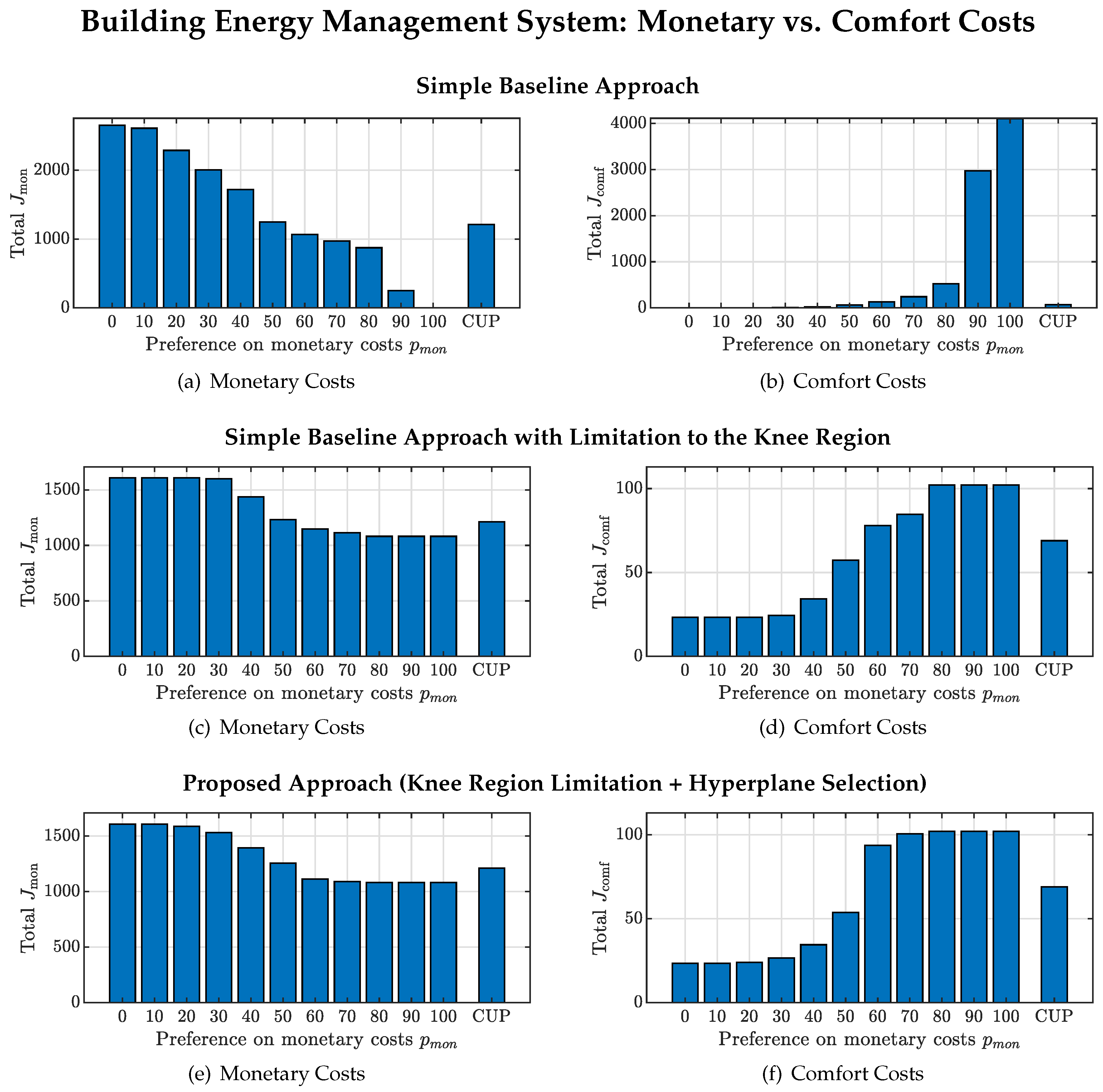
5.4.3. Simulation Results for 2 Objectives

For the 2D simulations, we vary $p_{\mathrm{mon}}$ from 0 to 100 while $p_{\mathrm{mon}}+p_{\mathrm{comf}}=100$. The results are shown in Figure 9.

Figure 9a,b show the monetary and comfort costs for the simple baseline approach. The preferences are respected, i.e., every increase in $p_{\mathrm{mon}}$ leads to a decrease in monetary costs and consequently to an increase in comfort costs. However, the trade-offs for higher preference values are extreme, especially the resulting comfort costs for $p_{\mathrm{mon}}\ge 80$.

This can be overcome by limiting all possible selections to the knee region as we propose. If so, even the simple selection shows good results in the 2D case; see Figure 9c,d. The highest comfort costs are limited to ≈100, instead of >4000. Note that for $p_{\mathrm{mon}}=\{0,10,20\}$ and $p_{\mathrm{mon}}=\{80,90,100\}$, respectively, the results are (nearly) the same, because the knee region sizes have been so small that the extremes are (nearly) almost chosen by rounding. This would be different for denser samplings.

The proposed approach (Figure 9e,f) incorporates the preferences in the long-term costs as expected, too. Furthermore, the knee region limitation leads to the same results for $p_{\mathrm{mon}}=\{0,10\}$ and $p_{\mathrm{mon}}=\{80,90,100\}$ only. However, here, this is not due to the sampling density and rounding but rather intended behavior. Namely, the resulting preference planes are so steep that they choose the extreme points of the knee region every time. Note that this would change for increasing knee region sizes, i.e., for $r_{\lim }<0.85$.

Concluding, in the 2D case, the simple baseline approach is inappropriate for the dynamic decision making due to choices and trade-offs which are too extreme if the preferences are not set cautiously. The limitation of possible selections to a knee region, i.e., the first step of our two-step approach, can overcome this problem even in combination with a simpler selection technique than the proposed preference hyperplane (the second step of our proposed approach). However, most likely, this only holds because the occurring Pareto fronts are all convex. Furthermore, in the following, we will see that the selection based on the preference hyperplane is superior if three objectives are considered.

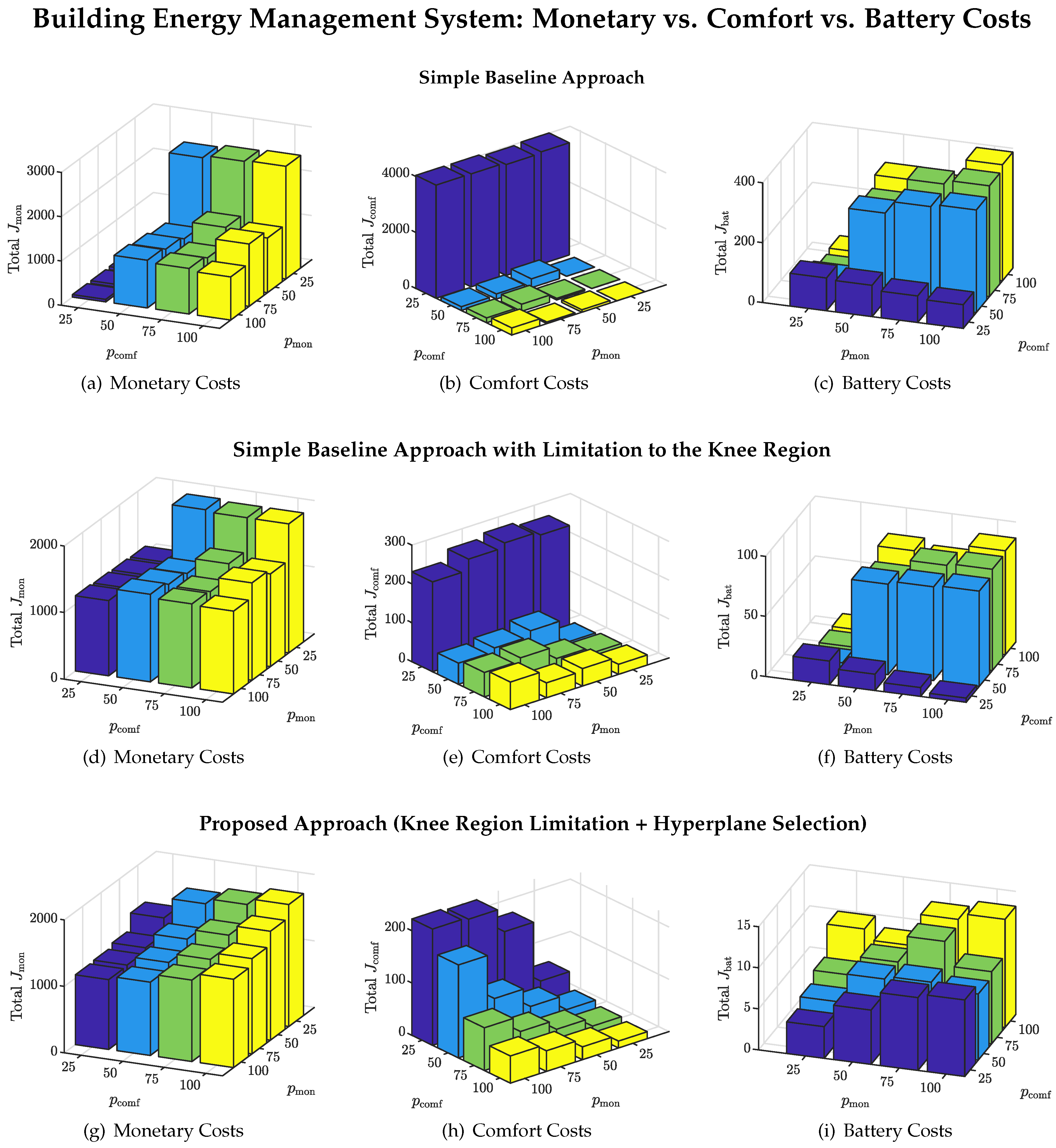
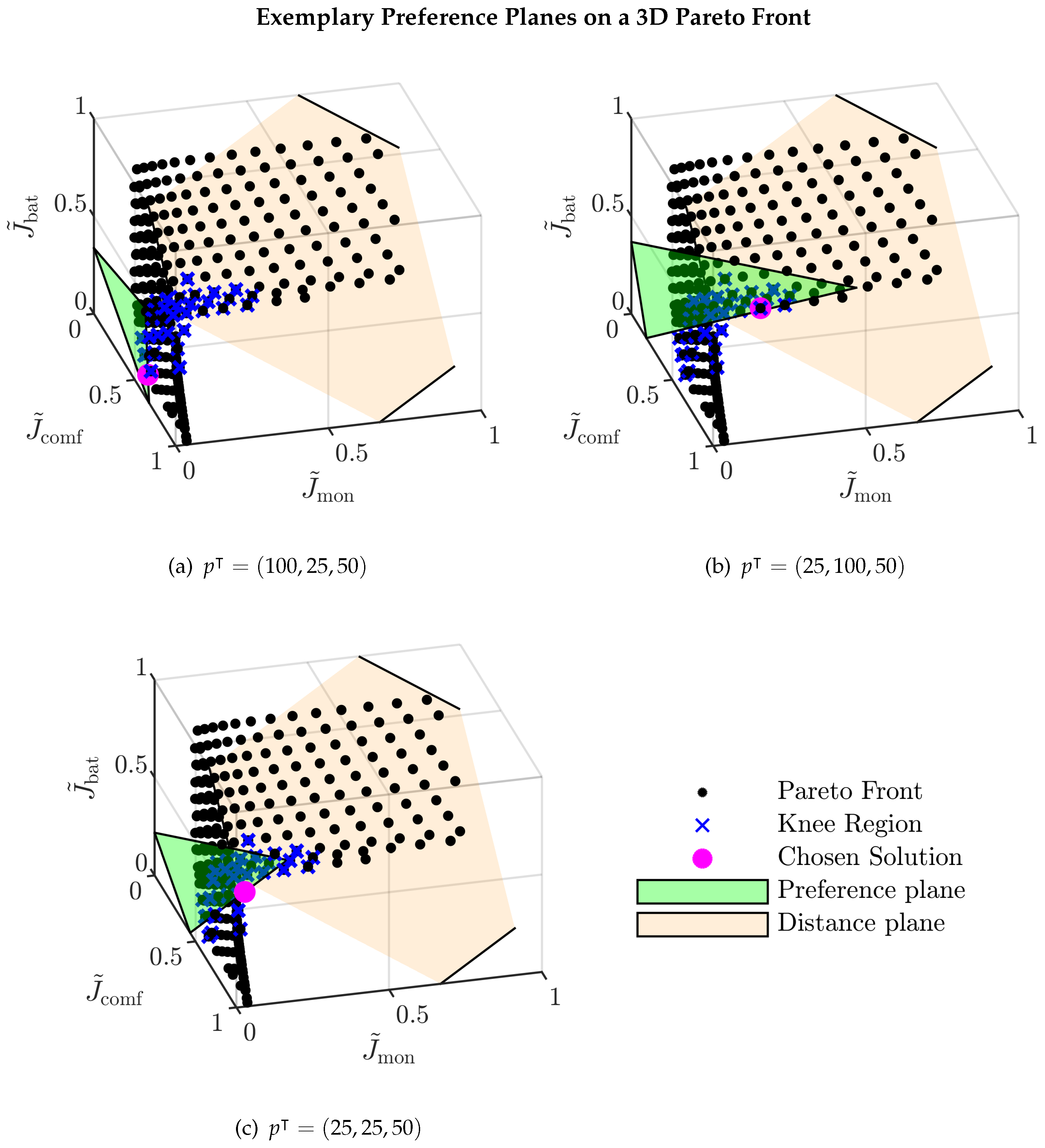
5.4.4. Simulation Results for 3 Objectives

The battery degradation costs are now considered as an additional third objective. Since only the relationship between the elements of the preference vector $p^{⊺}=(p_{\mathrm{mon}},p_{\mathrm{comf}},p_{\mathrm{bat}})$ is relevant, we vary both $p_{\mathrm{mon}}$ and $p_{\mathrm{comf}}$ as $\{25,50,75,100\}$, while we keep $p_{\mathrm{bat}}=50$ constant.

Figure 10a–c show the simulation results for the simple baseline approach. As in the 2D case, the costs for higher differences in the preferences become extreme, especially the comfort costs in Figure 10b. Furthermore, in contrast to the 2D case, the resulting long-term costs do not follow the preferences as expected. For example, in Figure 10a, the monetary costs are reduced by half first if preferences are changed from $\left(\begin{array}{ccc}{p}_{\mathrm{mon}},& p_{\mathrm{comf}},& p_{\mathrm{bat}}\end{array}\right)=\left(\begin{array}{ccc}25,& 100,& 50\end{array}\right)$ to $\left(\begin{array}{ccc}50,& 100,& 50\end{array}\right)$, but then, they increase for $\left(\begin{array}{ccc}75,& 100,& 50\end{array}\right)$. Note that these considerable jumps and changes in direction can partly be explained by the necessary ordering in the algorithm. Namely, the order in which the objectives are considered in removing parts of the Pareto front is relevant. For equal preferences of two objectives, $J_{\mathrm{mon}}$ is respected before $J_{\mathrm{comf}}$, which is respected before $J_{\mathrm{bat}}$. However, this does not explain all of the unwanted behavior. Consider the row for $p_{\mathrm{comf}}=50$ in Figure 10a. The monetary costs increase instead of decreasing if $p_{\mathrm{mon}}$ is increased from 50 to both 75 or 100, although the order in which the objectives are considered is the same, i.e., first $J_{\mathrm{mon}}$, then $J_{\mathrm{comf}}$ and then $J_{\mathrm{bat}}$. The battery costs in Figure 10c are even more turbulent. They decrease instead of increasing for increasing $p_{\mathrm{mon}}$ and $p_{\mathrm{comf}}=25$ and have drastic jumps in general.

Figure 10d–f show the simulation results for the simple baseline approach if the selection is limited to the knee region. As expected, the extreme solutions are avoided, i.e., the maximum comfort costs are reduced from $4040.14$ to $271.12$, and the battery costs are reduced from $387.56$ to $86.49$. However, the unwanted behavior is mostly the same otherwise. In contrast to the 2D case, the limitation to the knee region is not sufficient in combination with the simple baseline approach for an appropriate representation of the preferences in the long-term simulation costs.

Figure 10g–i show the simulation results for our proposed approach. In contrast to the baseline approach, the long-term costs for the monetary and comfort objective differ when varying $p_{\mathrm{mon}}$ and $p_{\mathrm{comf}}$, just as expected. The jumps between the different preference settings are smaller and more evenly distributed. Every increase in a preference leads to a decrease in the long-term costs and vice versa.

For the battery costs, some simulations still show unexpected results, e.g., the total $J_{\mathrm{bat}}$ is slightly lower for $p^{⊺}=\left(\begin{array}{ccc}100,& 50,& 50\end{array}\right)$ than for $p^{⊺}=\left(\begin{array}{ccc}100,& 75,& 50\end{array}\right)$. However, this can be explained by the weak influence of $J_{\mathrm{bat}}$. Battery and comfort costs are nearly independent and only implicitly linked via the monetary costs or possibly if $P_{\mathrm{grid}}$ would be at its limit. The monetary costs are in direct conflict with the battery costs because they can be reduced by buying energy at lower prices, storing it temporarily and selling it at higher prices. However, the assumed battery capacity and charging power are so low that the vast majority of possible monetary costs are due to the possible (but not necessary) cooling and heating of the building. Thus, the Pareto fronts become extremely steep, as Figure 11 exemplary shows. The Pareto fronts are almost degenerate [36].

However, our approach still handles this problem sufficiently well, as Figure 10i shows a clear trend of increasing costs $J_{\mathrm{bat}}$ from $p_{\mathrm{mon}}=p_{\mathrm{comf}}=25$ to $p_{\mathrm{mon}}=p_{\mathrm{comf}}=100$. Furthermore, in contrast to the baseline approach (even with the limitation to the knee region), the battery costs are significantly lower with a maximum of $13.18$ instead of $86.49$ overall. The long-term results can actually be considered better overall, as our approach outperforms both the simple approach e.g., $\left(\begin{array}{ccc}25,& 25,& 50\end{array}\right)$ vs. $\left(\begin{array}{ccc}75,& 100,& 50\end{array}\right)$ and the simple approach with prior limitation to the knee region e.g., $\left(\begin{array}{ccc}75,& 25,& 50\end{array}\right)$ vs. $\left(\begin{array}{ccc}55,& 25,& 50\end{array}\right)$ for some preference combinations.

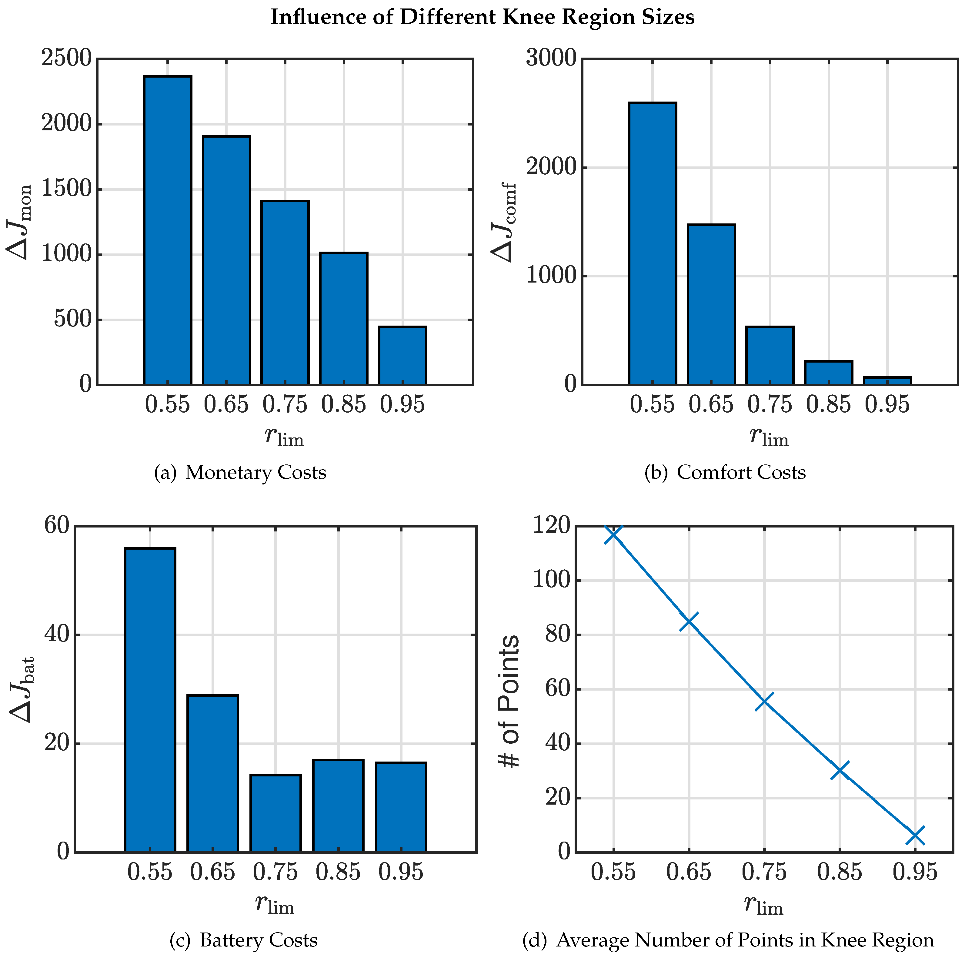
5.4.5. Influence of Knee Region Size

Figure 12 shows how $r_{\lim }$ affects the possible influence of the decision maker. For every $r_{\lim }$, we simulated the three possible extremes $p^1={(1,0,0)}^{⊺}$, $p^2={(0,1,0)}^{⊺}$ and $p^3={(0,0,1)}^{⊺}$ and calculated the maximum difference for each objective, e.g.,

$$\Delta J_{\mathrm{mon}}(r_{\lim })=\underset{p\in \{p^2,p^3\}}{max}(J_{\mathrm{mon}}(r_{\lim },p))-J_{\mathrm{mon}}(r_{\lim },p^1).$$

(45)

The difference in monetary costs shown in Figure 12a is nearly (anti)proportional to $r_{\lim }$. The possible differences $\Delta J_{\mathrm{comf}}$ seem to decrease quadratically with an increasing $r_{\lim }$ in Figure 12b, which is probably due to its quadratic form (42). The battery costs in Figure 12c again have an outlier for $r_{\lim }=0.75$, which can be explained by its bad conditioning in comparison to $J_{\mathrm{comf}}$ as discussed before. However, the trend of the decrease in $\Delta J_{\mathrm{bat}}$ with an increasing $r_{\lim }$ is clear, too. The average number of Pareto points which are determined as part of the knee region correlates nearly linear to $r_{\lim }$, as Figure 12d shows. However, this depends on the shapes of the Pareto fronts and cannot be generalized.

6. Conclusions

We presented a two-step approach for automated decision making from an available Pareto front. It allows a decision maker to formulate the preferences of each objective independently of their scales. At the same time, it (1) ensures that only good compromises can be selected by limiting possible choices to a knee region, which (2) depends on the Pareto front’s shape, (3) gives the decision maker a design parameter with which he can comprehensibly choose a priori how strong his influence should be, and (4) has a built-in proclivity for knee points, if they exist. Thus, it enables the use of MOO in continuous processes where decisions have to be made repeatedly, such as in multi-objective (economic) MPC, where varying circumstances may lead to very different possible decisions regularly. The simulation results of a toy example as well as a more sophisticated case study of a building energy management system showed superior results in comparison to simpler selection techniques especially for $n=3$ objectives.

References

1. Schmitt, T.; Engel, J.; Rodemann, T.; Adamy, J. Application of Pareto Optimization in an Economic Model Predictive Controlled Microgrid. In Proceedings of the 2020 28th Mediterranean Conference on Control and Automation (MED), Saint-Raphaël, France, 15–18 September 2020; pp. 868–874. [Google Scholar] [CrossRef]
2. Schmitt, T.; Rodemann, T.; Adamy, J. Multi-objective model predictive control for microgrids. at-Automatisierungstechnik 2020, 68, 687–702. [Google Scholar] [CrossRef]
3. Azzouz, R.; Bechikh, S.; Ben Said, L. Dynamic Multi-objective Optimization Using Evolutionary Algorithms: A Survey. In Recent Advances in Evolutionary Multi-Objective Optimization; Springer International Publishing: Cham, Switzerland, 2017; pp. 31–70. [Google Scholar] [CrossRef]
4. Ghosh, A.; Dehuri, S. Evolutionary Algorithms for Multi-Criterion Optimization: A Survey. Int. J. Comput. Inf. Sci. 2004, 2, 38. [Google Scholar]
5. Zitzler, E.; Laumanns, M.; Bleuler, S. A tutorial on evolutionary multiobjective optimization. In Metaheuristics for Multiobjective Optimisation; Springer: Berlin/Heidelberg, Germany, 2004; pp. 3–37. [Google Scholar]
6. Gembicki, F.; Haimes, Y. Approach to performance and sensitivity multiobjective optimization: The goal attainment method. IEEE Trans. Autom. Control. 1975, 20, 769–771. [Google Scholar] [CrossRef]
7. Pascoletti, A.; Serafini, P. Scalarizing vector optimization problems. J. Optim. Theory Appl. 1984, 42, 499–524. [Google Scholar] [CrossRef]
8. Das, I.; Dennis, J.E. Normal-boundary intersection: A new method for generating the Pareto surface in nonlinear multicriteria optimization problems. SIAM J. Optim. 1998, 8, 631–657. [Google Scholar] [CrossRef] [Green Version]
9. Motta, R.d.S.; Afonso, S.M.; Lyra, P.R. A modified NBI and NC method for the solution of N-multiobjective optimization problems. Struct. Multidiscip. Optim. 2012, 46, 239–259. [Google Scholar] [CrossRef]
10. Ghane-Kanafi, A.; Khorram, E. A new scalarization method for finding the efficient frontier in non-convex multi-objective problems. Appl. Math. Model. 2015, 39, 7483–7498. [Google Scholar] [CrossRef]
11. Messac, A.; Ismail-Yahaya, A.; Mattson, C.A. The normalized normal constraint method for generating the Pareto frontier. Struct. Multidiscip. Optim. 2003, 25, 86–98. [Google Scholar] [CrossRef]
12. Mueller-Gritschneder, D.; Graeb, H.; Schlichtmann, U. A successive approach to compute the bounded Pareto front of practical multiobjective optimization problems. SIAM J. Optim. 2009, 20, 915–934. [Google Scholar] [CrossRef]
13. Srinivasan, V.; Shocker, A.D. Linear programming techniques for multidimensional analysis of preferences. Psychometrika 1973, 38, 337–369. [Google Scholar] [CrossRef]
14. Zavala, V.M. Real-time optimization strategies for building systems. Ind. Eng. Chem. Res. 2013, 52, 3137–3150. [Google Scholar] [CrossRef] [Green Version]
15. Hwang, C.L.; Yoon, K. Multiple Attribute Decision Making: Methods and Applications, 1st ed.; Lecture Notes in Economics and Mathematical Systems 186; Springer: Berlin/Heidelberg, Germany, 1981. [Google Scholar]
16. Miettinen, K. Nonlinear Multiobjective Optimization; Springer Science & Business Media: New York, NY, USA, 1999; Volume 12. [Google Scholar]
17. Jin, Y.; Sendhoff, B. Incorporation Of Fuzzy Preferences Into Evolutionary Multiobjective Optimization. In Proceedings of the GECCO, New York, NY, USA, 9–13 July 2002; Volume 2, p. 683. [Google Scholar]
18. Farina, M.; Amato, P. A fuzzy definition of "optimality" for many-criteria optimization problems. IEEE Trans. Syst. Man Cybern.-Part A Syst. Humans 2004, 34, 315–326. [Google Scholar] [CrossRef]
19. Yang, J.B.; Xu, D.L. On the evidential reasoning algorithm for multiple attribute decision analysis under uncertainty. IEEE Trans. Syst. Man Cybern.-Part A Syst. Hum. 2002, 32, 289–304. [Google Scholar] [CrossRef] [Green Version]
20. Li, Y.; Liao, S.; Liu, G. Thermo-economic multi-objective optimization for a solar-dish Brayton system using NSGA-II and decision making. Int. J. Electr. Power Energy Syst. 2015, 64, 167–175. [Google Scholar] [CrossRef]
21. Branke, J.; Deb, K.; Dierolf, H.; Osswald, M. Finding knees in multi-objective optimization. In Proceedings of the International Conference on Parallel Problem Solving from Nature, Birmingham, UK, 18–22 September 2004; Springer: Cham, Switzerland, 2004; pp. 722–731. [Google Scholar]
22. Deb, K.; Gupta, S. Understanding knee points in bicriteria problems and their implications as preferred solution principles. Eng. Optim. 2011, 43, 1175–1204. [Google Scholar] [CrossRef]
23. Braun, M.; Shukla, P.; Schmeck, H. Angle-Based Preference Models in Multi-objective Optimization. In Proceedings of the Evolutionary Multi-Criterion Optimization, Münster, Germany, 19–22 March 2017; Trautmann, H., Rudolph, G., Klamroth, K., Schütze, O., Wiecek, M., Jin, Y., Grimme, C., Eds.; Springer International Publishing: Cham, Switzerland, 2017; pp. 88–102. [Google Scholar]
24. Bechikh, S.; Said, L.B.; Ghédira, K. Searching for knee regions of the Pareto front using mobile reference points. Soft Comput. 2011, 15, 1807–1823. [Google Scholar] [CrossRef]
25. Rachmawati, L.; Srinivasan, D. Multiobjective evolutionary algorithm with controllable focus on the knees of the Pareto front. IEEE Trans. Evol. Comput. 2009, 13, 810–824. [Google Scholar] [CrossRef]
26. Bhattacharjee, K.S.; Singh, H.K.; Ryan, M.; Ray, T. Bridging the Gap: Many-Objective Optimization and Informed Decision-Making. IEEE Trans. Evol. Comput. 2017, 21, 813–820. [Google Scholar] [CrossRef]
27. Yu, G.; Jin, Y.; Olhofer, M. A Method for a Posteriori Identification of Knee Points Based on Solution Density. In Proceedings of the 2018 IEEE Congress on Evolutionary Computation (CEC), Rio de Janeiro, Brazil, 8–13 July 2018; pp. 1–8. [Google Scholar] [CrossRef]
28. Das, I. On characterizing the “knee” of the Pareto curve based on normal-boundary intersection. Struct. Optim. 1999, 18, 107–115. [Google Scholar] [CrossRef]
29. Li, W.; Wang, R.; Zhang, T.; Ming, M.; Li, K. Reinvestigation of evolutionary many-objective optimization: Focus on the Pareto knee front. Inf. Sci. 2020, 522, 193–213. [Google Scholar] [CrossRef]
30. Molina, J.; Santana, L.V.; Hernández-Díaz, A.G.; Coello Coello, C.A.; Caballero, R. g-dominance: Reference point based dominance for multiobjective metaheuristics. Eur. J. Oper. Res. 2009, 197, 685–692. [Google Scholar] [CrossRef]
31. Hu, J.; Yu, G.; Zheng, J.; Zou, J. A preference-based multi-objective evolutionary algorithm using preference selection radius. Soft Comput. 2017, 21, 5025–5051. [Google Scholar] [CrossRef]
32. Deb, K.; Miettinen, K.; Sharma, D. A hybrid integrated multi-objective optimization procedure for estimating nadir point. In Proceedings of the 5th International Conference, EMO 2009, Nantes, France, 7–10 April 2009; Springer: Berlin/Heidelberg, Germany, 2009; pp. 569–583. [Google Scholar]
33. Wang, Y.; Limmer, S.; Olhofer, M.; Emmerich, M.; Bäck, T. Automatic Preference Based Multi-objective Evolutionary Algorithm on Vehicle Fleet Maintenance Scheduling Optimization. Swarm Evol. Comput. 2021, 65, 100933. [Google Scholar] [CrossRef]
34. Das, I.; Dennis, J.E. A closer look at drawbacks of minimizing weighted sums of objectives for Pareto set generation in multicriteria optimization problems. Struct. Optim. 1997, 14, 63–69. [Google Scholar] [CrossRef] [Green Version]
35. Ryu, N.; Min, S. Multiobjective optimization with an adaptive weight determination scheme using the concept of hyperplane. Int. J. Numer. Methods Eng. 2019, 118, 303–319. [Google Scholar] [CrossRef]
36. Hua, Y.; Liu, Q.; Hao, K.; Jin, Y. A Survey of Evolutionary Algorithms for Multi-Objective Optimization Problems With Irregular Pareto Fronts. IEEE/CAA J. Autom. Sin. 2021, 8, 303–318. [Google Scholar] [CrossRef]
37. De Vito, D.; Scattolini, R. A receding horizon approach to the multiobjective control problem. In Proceedings of the 2007 46th IEEE Conference on Decision and Control, New Orleans, LA, USA, 12–14 December 2007; pp. 6029–6034. [Google Scholar]
38. Bemporad, A.; de la Peña, D.M. Multiobjective model predictive control. Automatica 2009, 45, 2823–2830. [Google Scholar] [CrossRef]
39. Zavala, V.M.; Flores-Tlacuahuac, A. Stability of multiobjective predictive control: A utopia-tracking approach. Automatica 2012, 48, 2627–2632. [Google Scholar] [CrossRef]
40. Schmitt, T.; Engel, J.; Hoffmann, M.; Rodemann, T. PARODIS: One MPC Framework to control them all. Almost. In Proceedings of the 2021 IEEE Conference on Control Technology and Applications (CCTA), San Diego, CA, USA, 9–11 August 2021. [Google Scholar]
41. Di Somma, M.; Yan, B.; Bianco, N.; Graditi, G.; Luh, P.; Mongibello, L.; Naso, V. Multi-objective design optimization of distributed energy systems through cost and exergy assessments. Appl. Energy 2017, 204, 1299–1316. [Google Scholar] [CrossRef]
42. Moghaddam, A.A.; Seifi, A.; Niknam, T.; Alizadeh Pahlavani, M.R. Multi-objective operation management of a renewable MG (micro-grid) with back-up micro-turbine/fuel cell/battery hybrid power source. Energy 2011, 36, 6490–6507. [Google Scholar] [CrossRef]
43. Schmitt, T.; Rodemann, T.; Adamy, J. The Cost of Photovoltaic Forecasting Errors in Microgrid Control with Peak Pricing. Energies 2021, 14, 2569. [Google Scholar] [CrossRef]
44. Engel, J.; Schmitt, T.; Rodemann, T.; Adamy, J. Hierarchical Economic Model Predictive Control Approach for a Building Energy Management System With Scenario-Driven EV Charging. IEEE Trans. Smart Grid 2022, 13, 3082–3093. [Google Scholar] [CrossRef]
Figure 1. Illustration of the presented approach in the automatized decision making process for multi-objective MPC. As usual in MPC, at every time step, an optimization problem (i.e., an optimal control problem) over some time horizon is formulated. Here, the multiple objectives lead to a multi-objective optimal control problem. The result is a new Pareto front (at every time step) from which a solution has to be chosen. In our approach, we first identify reasonable areas of the Pareto front, i.e., we exclude too extreme solutions. Then, we incorporate the decision maker’s preferences to finally choose a compromise. The solution represents a control (input) plan which is then applied to the system (at least the first step in case of MPC). Afterwards, the resulting system state is measured, and the process is repeated for the next time step.
Inventions 07 00046 g001
Figure 2. Exemplary knee regions in 2D for different r lim . For fronts without a knee point (a), the knee region is larger than for fronts with a knee point (b) for any r lim . Note that for convex 2D fronts, the distance plane is equivalent to the convex hull of the minima from [28] (if normalized).
Inventions 07 00046 g002
Figure 3. Flowchart diagram for the first step of the proposed decision making approach, i.e., the determination of the knee region.
Inventions 07 00046 g003
Figure 4. Exemplary preference planes (12) for the Pareto fronts from Figure 2 and r lim = 0.8 . Note that for the front without a knee in (a), the different preferences lead to solutions far apart from each other. For the front with a knee in (b), two of the three preferences choose the knee itself. Even for p = [ 0.75 , 0.25 ] , the selected solution is close to the knee point, despite the large knee region (with solutions a human decision maker would not consider interesting).
Inventions 07 00046 g004
Figure 5. Flowchart diagram for the second step of the proposed decision making approach, i.e., the final selection of a solution from the knee region.
Inventions 07 00046 g005
Figure 6. Comparison of the knee regions and selections for the artifical Pareto front from (14) for various underestimated J extreme , 2 and three different preference settings. r lim = 0.85 . As expected, both the knee region and the final decision shift to the right, i.e., to higher values of J 1 , for lower J extreme , 2 . The shift is more severe for higher preferences on J 2 (see magenta square). (a) Complete Pareto front with J extreme , 2 = 1000.50 , (bf) incomplete Pareto fronts with underestimated J extreme , 2 from 750 to 50.
Inventions 07 00046 g006
Figure 7. High-level flowchart diagram of the focus point boundary intersection method. Note that the unnormalized Pareto solutions J can be derived from J ˜ by rearranging (8).
Inventions 07 00046 g007
Figure 9. Monetary and comfort costs for the 30-day 2D simulations with different preferences p mon and p comf for (a,b) the simple baseline approach, (c,d) the simple baseline approach but with limitation to the knee region, and (e,f) the proposed preference-based decision making approach, with r lim = 0.85 for the latter two cases. Results from using the closest to Utopia point (CUP) metric are plotted for comparison.
Inventions 07 00046 g009
Figure 10. Monetary, comfort and battery degradation costs for the 30 days of 3D simulations with different preferences p mon and p comf and p bat = 50 for (ac) the simple baseline approach and (df) the simple baseline approach but with limitation to the knee region and (gi) the proposed preference-based decision making approach, with r lim = 0.85 for the latter two cases. Note the different camera angles for better readability and especially the inverted axis for p comf in (c,f,i). Subtracted minimum costs for each objective have been determined by single-objective optimizations.
Inventions 07 00046 g010
Figure 11. Single Pareto front from simulation with its knee region ( r lim = 0.85 ) and different preference planes with focus on (a) monetary, (b) comfort and (c) battery costs. Note that the different preferences are according to the extreme cases from Figure 10.
Inventions 07 00046 g011
Figure 12. Maximum difference in total monetary (a), comfort (b) and battery (c) costs and the average number of points considered to be part of the knee region (d) for different r lim , which were calculated according to (45).
Inventions 07 00046 g012
Publisher’s Note: MDPI stays neutral with regard to jurisdictional claims in published maps and institutional affiliations.