Article

Numerical Investigation of Winglet Aerodynamics and Dimple Effect of NACA 0017 Airfoil for a Freight Aircraft

by
Matthew Thomas Lewthwaite
1,* and
Chiemela Victor Amaechi
1,2,*
1
Department of Engineering, Lancaster University, Lancaster LA1 4YR, UK
2
Standardisation Directorate, Standard Organisation of Nigeria (SON), 52 Lome Crescent, Wuse Zone 7, Abuja 900287, Nigeria
*
Authors to whom correspondence should be addressed.
Inventions 2022, 7(1), 31; https://doi.org/10.3390/inventions7010031
Submission received: 11 December 2021 / Revised: 19 February 2022 / Accepted: 21 February 2022 / Published: 7 March 2022
(This article belongs to the Special Issue New Advances and Challenges in Wind Energy Extraction II)

Abstract

:
Drag reduction is an ever-present challenge within the aeronautical engineering industry. This paper presents two substantial wing modifications: the addition of a winglet of a freighter aircraft and a dimpled wing on the NACA 0017 aerofoils. Studies on nine (9) different geometries of dimpled aerofoils were performed against a control model of an aerofoil without any dimple. Computational fluid dynamics (CFD) analysis was performed using two (2) commercial CFD platforms. This paper also explored two novel solutions of aircraft optimisation to mitigate the effects of drag and leading-edge pressure, while increasing the effect of lift. The optimised performance model of a freighter aircraft increased its aerodynamic efficiency. The study found that at take-off velocity of 82 m/s, winglets decreased pressure on the wing by 16.31%, through flow redirection and better flow integration into aerofoils wake. The study also analysed the separation layer and its effect through the appropriate use of the dimple effect. Increased lift effects were observed on a NACA 0017 aerofoil. Despite the low increase in drag of 6% from the modifications, the resultant L/D ratio was highly increased. This study also faced some challenges with validating the model. Hence some validation approaches were taken, and some other approaches suggested for future studies.

1. Introduction

Current trends in the research on dimples show aerodynamic effects on a variety of applications, such as golf balls, wind turbine blades, and aircraft wings (for military, cargo, passenger, or freighter aircrafts). Freighter aeroplanes serve public, government, and private sectors, delivering different goods and services across the continents. Air transportation is the quickest means of transport globally today. Aeroplanes, which are energy-powered flying vehicles whose wings are fixed, and the mass is greater than that of the displaced air [1] are not the only means of air transport. Others include helicopters, aircrafts, drones, stealth crafts, fighter jets, etc. These serve other purposes for logistics, military supplies, or distributing small, electronic components. Amazon, a global logistics company, has achieved current drone delivery applications for supplying goods [2]. Also, drones have been deployed for organ transplant in the University of Maryland Medical Center, USA [3,4] There are other applications of aviation crafts, such as military fighter jets, and stealth jets. Fast jets are typically required to respond to a combat situation as quickly and effectively as possible. Due to the application, they must be smaller with delicate parts to increase aerodynamic efficiency. They usually house a delta-shaped wing to increase agility in air-to-air combat [5], using an aerodynamically efficient aeroplane [6].
By size, the specification of the freighter aircraft results in a large cargo capacity, which is the most critical factor when considering their design. The Antonov An-225 Mriya’s wingspan of 88.4 metres [7] is nine times (9×) larger than the wingspan of the F-16 Fighting Falcon [8]. The Antonov’s wings are situated at the top of the fuselage to maximise the fuselage’s storage capacity. The wings slope to optimise the aircraft’s ability to glide; this consequently reduces fuel consumption. A smaller, fast jet has less exposed surface area and will experience less drag than a freighter aircraft when travelling at the same velocity and altitude [9]. One drag reduction method is to increase the aspect ratio of a wing. However, there are two immediate limitations on the length of an aircraft’s wingspan. One restriction is imposed by airports globally, for they do not have the room nor the runway width to adhere to the needs of an extended wing length. The second is imposed by the structural capability of the wing’s materials. Early aircrafts, such as the Wright Brothers Flyer, used wood as their primary construction material. Although this initially seems to be a primitive construct, an omen to the early days of material science, the use of wood to fabricate major aircraft components is present throughout the 1940s. This design feature is prominent in the De Havilland Mosquito, first conceived in November of 1940, flying throughout World War Two (WW2) [10]. For any full-size modern aircraft, aluminium is wood’s successor. While wood has a high strength to weight ratio, aluminium’s is considerably higher, without the long production process of drying and lamination. Aluminium alloys are also more resistant to erosion and more accessible to fabricate when compared to wood. Aluminium’s increased strength means it is structurally more capable than wood and can bare a larger wing load. In principle, aircraft wings can be described as cantilever beam; only supported at one end, the bending moment at the wing tip will be larger than the bending moment of the wing at the fuselage. The longer the wing, the larger the resulting bending moment and the more support the wing will need. Aluminium can provide the desired level of support, above most airport width restrictions. It, therefore, follows that adhering to airport demands is the primary restriction on aircrafts.
In regard to the effect of dimple on the aerofoil, different studies that include the dimple geometry, the angle of attack (AOA) and the inlet velocity have been considered by various researchers. The implementation of the dimple effect can be used to reduce the size of the vortex in the wake of the aerofoil can be reduced. The dimple effect is a drag reduction method, most notable for its appearance on golf balls. When the flow follows the impressions on the surface of the golf ball, the elevation changes induced by the dimple, thereby creating an extension to the boundary layer. As the flow progresses along with the golf ball, the low pressure in the boundary layer seeks equilibrium, effectively sucking in the surrounding high-pressure flow. This attempt to balance pressure allows the airflow surrounding the ball to travel closer to its surface and follow its shape for longer. The tighter airflow produces a reduction in the size of the vortex found in the wake of the ball [11]. However, the vortex phenomenon occurs in different fluid medium, both in air and water. An earlier study conducted in 1945 discovered that with a standard dimple depth of 0.254 mm, the ball experienced a 25% reduction in drag when compared to a smooth surfaced ball [12]. The author concluded that dimple depth also affected performance, with balls that house shallower impressions experiencing marginal or no aerodynamic improvement. Golf ball manufacturers have started to vary dimple geometry and patterns to optimise ball performance. Experiments have been conducted that compare the standard design to elliptical and hexagonal impressions.
One objective of this study is to determine the dimple effect phenomenon and to implement it by optimising aircraft wings. Despite little research on this, evidence from existing experiments on dimple spread, pattern, and the number of dimples present on the surface can vary drag results by up to 40% [13]. Arunkumar et al. [14] investigated dimples with a diameter of 0.2 c on the top of an aerofoil operating at 10° AOA. The study found that a semi-circular dimple geometry was optimum, increasing the lift efficiency coefficient by 0.73, and 30.8%. In another research by Soh and Al-Obai [15], simulations were conducted on a NACA 0012 aerofoil in which dimples of varying geometries were placed at 0.2 c, both on the top and the bottom of the aerofoil. When the results were compared against a smooth aerofoil with an inlet speed of 10 m/s, it was found that an elliptical dimple located on the bottom of the wing, having a depth of 0.03125 C increased aerodynamic efficiency by 6.42% at 5° AOA, and 3% at 10° AOA. This study concludes that dimples on the underside of the aerofoil are more effective than those placed on top. While both modifications resulted in aerodynamic improvement, the variation in results can be explained using Bernoulli’s principle, which states that ‘velocity is inversely proportional to pressure’. Thus, pressure underneath the aerofoil is more significant than that on top. It follows that a dimple located underneath the aerofoil will experience more pressure because of the surrounding flow. Consequently, the dimple has more potential to increase lift and decrease drag [15].
Different numerical methods have been utilized on aerofoils, such as turbulence SST k-omega [16,17]. Simulations have also been conducted on the effects of a dimple pattern on the fuselage [18]. In this study, dimples were positioned at the second half of the fuselage after the flow had become more laminar. Therefore, the turbulent flow that the dimples induced resulted in drag being increased by 30%. There is potential for this concept to be improved if the dimple pattern could be relocated to the plane’s nose. To become more effective, dimples can be placed on the separation point of the aerofoil [19]. A separation point occurs when the boundary layer develops further, and the eddies contained within start to experience flow reversal [20]. After the separation point, the size of the boundary layer begins to increase, eventually leading to the formation of a turbulent wake. Consequently, this directs the flow reversal point towards the trailing edge, decreases the wake’s size behind the aerofoil, and subsequently decreases drag. For most symmetrical aerofoils at 0° AOA (angle of attack), a separation point occurs towards the trailing edge of the aerofoil, as AOA increases the separation towards the leading edge [21,22]. Figure 1 shows an illustration depicting the constituent forces acting on dimpled aerofoils, including its Angle of attack (AOA).
This paper investigates the flow behaviour on a winglet and the dimple effect on aircraft wings to determine separation points that can be applied to improve aircraft performance. To understand the flow progression over an aerofoil, the formation of a boundary layer and the subsequent separation point over a NACA 00017 aerofoil at 0° AOA has been conducted with details on the interaction of airflow around aerofoil. Section 1 introduces the research, while Section 2 presents some fundamental theories on the investigation. The study results are presented in Section 3, and some discussions are made in Section 4. Concluding remarks are made in Section 5.

2. Numerical Model

2.1. The Fundamental Theory

2.1.1. Aerodynamic Forces

There are different forces that can influence the performance and aerodynamics of the aircrafts. These range from the viscous force, motor force, drag force, weight of the aircraft, wing geometry, turbulence, and other forces. However, the effect of drag force will be analysed in this study, as this has been found to affect the performance greatly. The drag force is as a result of the combined effects of pressure and wall shear forces. The drag force can be expressed mathematically by Equation (1), where, Cd is the drag coefficient, ρ is the density of air, V is the flow velocity relative to the aircraft, and A is the cross-sectional area of the wing. However, there is a need to increase the power of the commercial van to make it more efficient. To obtain the power (P) required to overcome this drag, we consider the expression in Equation (2) where the drag coefficient is proportional to the cube of the velocity (V).
F D = 1 2 C d ρ V 2 A
P = 1 2 ρ C d A V 3

2.1.2. Air Flow Theories

The airflow around the freight aircrafts is high-speed aerodynamics; thus, the airflow field can be regarded as three-dimensional (3D) compressible flow. However, in the present study, the focus is on an aerofoil and a weightless winglet. The fundamental governing equations for the three-dimensional incompressible flow are presented in this section. The Navier–Stokes equation was applied with the K- ω or k- ε turbulence model to solve the compressible airflow. Navier–Strokes equations consist of governing equations, such as the Continuity equation (see Equation (3)) and Momentum equations (see Equations (4)–(6)), where u, v, and z are the components of velocity vector in x, y, and z-components; ρ is the air density, P0 is static pressure, and Sm,x, Sm,y, and Sm,z are source terms for x, y, and z components. On the left hand side of Equations (3)–(6), the first term is a density gradient. Also, on the right hand side of Equations (3)–(6), the first term is a pressure gradient. It should be noted that the Navier–Stokes Equations (3)–(6) are not incompressible since it involves density variation. Hence, they are expressed herein since they are compressible but should have the required energy equation as in Equations (4)–(6). Thus, we have:
ρ t + 𝛻 ( p V ) = 0
ρ ( u E T ) t + 𝛻 ( ρ u V ) = p x + 𝛻 ( μ 𝛻 u ) + S m , x
ρ ( vE T ) t + 𝛻 ( ρ v V ) = p y + 𝛻 ( μ 𝛻 v ) + S m , y
ρ ( w E T ) t + 𝛻 ( ρ w V ) = p z + 𝛻 ( μ 𝛻 w ) + S m , z

2.1.3. Governing Equations for Aerofoils

Equations (7) and (8) show the normal and axial forces on top of the aerofoil, respectively, and Equations (9) and (10) display the respective forces underneath the aerofoil [22]. Figure 1 shows an illustration depicting the constituent forces acting on dimpled aerofoils.
d N u = ( p u c o s θ τ u s i n θ ) d s u
d A u = ( p u s i n θ τ u c o s θ ) d s u
d N l = ( p l c o s θ τ l s i n θ ) d s l    
d A l = ( p l s i n θ τ l c o s θ ) d s l

2.2. Turbulence Modelling

The SST k- ω (shear stress transport) turbulence model [16,17] was used to model the turbulent flow with automatic wall function. There are several considerations to make when selecting an appropriate turbulence model, the primary affecting factor of which is flow type. The simulations throughout this study were solved using the SST k- ω model. This model type utilizes the functions found in two independent models, k- ε and k- ω , and combines their calculations to obtain a more stable and therefore, reliable result, as presented in the Equations (11)–(15). As the intensity of the eddy currents at the inlet of two independent simulations can never be modelled identically, varying flows in the free stream change and effect overall results.
The SST k- ω model uses the accuracy of the k- ε to resolve values in the free stream where there is a constant flow type and use the k- ω model to solve near the wall of the object where Reynold number changes [16,17]. This is achieved by adding a blending function, F 1 [23]. A value of F 1 = 1 is given to the cells within the boundary layer. This will cancel ( 1 F 1 ) and the equation will be solved using the k- ω model, producing accurate, near-wall results. If F 1 = 0 , then ( 1 F 1 ) = 1 indicating flow is in the free stream, and the governing equations for the k- ε equation will be utilized [23]. The SST k- ω model also includes a near all viscosity limiter that limits the freeflow behaviour of the fluid. This replicates effects found within the Boussinesq’s turbulence hypothesis, which states that the prominent eddies found within a highly turbulent fluid alter the way momentum is transferred, causing the fluid to behave as if it were vicious.
ε ˜ t = y { ( v k v + v t σ ε ) ε ˜ y } + C 1 f 1 v t ε ˜ k ( u y ) 2 C 2 f 2 ε ˜ 2 k + E
f 1 = 1
f 2 = 1 0.3 e x p ( R e T 2 )
( ρ k ) t + ( ρ u j k ) x = p β * ρ ω k + x [ ( μ + σ k ρ k ω ) k x ]
ω t + u j ω x = α S 2 β ω 2 + x [ ( ν k v + σ ω ν t ) ω x ] + 2 ( 1 F 1 ) σ ω 2 1 ω k t x ω x

2.3. Aerofoil Geometry

To accurately model this wing and its curvature, aerofoil cross-sections were taken from several points along the wing’s length, from the root aerofoil to the wingtip. Data points for each NACA 0017 aerofoil were downloaded from [24], where they were lofted together to create a CAD model of the wing shown in Figure 2.
The three distinct winglets in Figure 2a–c were then designed in comparison to the normal Boeing 787-9 Dreamliner wings in Figure 2d, with the hypothesis that the delta-shaped winglets yield the highest percentage in drag reduction. Details of the parameters are presented in Table 1 and Table 2. The wing geometry for this study was modelled on the Boeing 787-9 Dreamliner aircraft and designed in Autodesk Inventor Professional 2019 CAD software. The Boeing 787-9 Dreamliner is a long-haul aircraft [25], with a total wingspan of 60 m, a root chord length of 13.5 m, a range of 14,010 km [26], and a take-off weight of 254,011 kg [27], as presented in Table 1.
The geometrical designs for the dimples and their location along the aerofoil are found in Figure 3. In turn each dimple geometry (ellipse, triangle, square) was placed atop, underneath and both on top and underneath the aerofoil. The dimensions of the dimples are shown in Table 2.
Aerofoil geometry is primarily governed by the structural requirements of the entire wing [28]. Thicker aerofoils are typically found on larger aircraft as they can accommodate a larger spar. A larger spar increases resistance to bending stress, something that is more prominent on longer wings, as shown in Equation (16), as in the literature [29]. Inherently, structural support is more beneficial for aerodynamic performance despite the elevated level of drag larger aerofoils create [28]. As a secondary point, aircraft fuel tanks are housed in the wing, and a larger spar has a larger area, so it can accommodate more fuel as needed for lengthy flights. Adhering to these parameters, the thicker NACA 0017 aerofoil was selected for this part of the study. The dimples were selected to be placed at 0.92 c, given that this is approximately where the separation point over the NACA 0017 aerofoil is located. This location was experimentally obtained and validated with literature from Anyoji, et al. [21].
M m a x i m u m = E I d 2 x d x 2

2.4. Methodology of CFD Analysis

The CFD model of different geometries, as discussed in Section 2.2, was created using CAD software. The model was modified to suit the geometry for the CFD model by importing the model to the Autodesk CFD 2019 software. Some mesh refinements in the CFD model were performed to define the geometry due to the dimple type for the NACA 0017 aerofoil. Figure 3 shows the arrangements along with each dimple geometry. The modifications of small sizes, like edges, gaps, and shape were performed, for the three design concepts-triangular, square, and elliptical (round) shapes. 50 time-consuming simulations were conducted to obtain a stable value for static pressure. Regarding this study, three recognisable dimple geometries were cut out of the aerofoil: an ellipse (round), a square and a triangle. A common depression depth of 0.021 c and a width of 0.032 c was selected. This value was determined by considering the studies previously mentioned and a need to preserve the structural integrity of the aerofoil. Each dimple shape is located underneath the aerofoil and then compared to the effects of a dimple located on the top, and a dimple located on both the top and underneath of the aerofoil. This design concept was conducted to evaluate the combined effects of the dimples. Figure 4 represents the setup for the aerodynamic properties in SimScale platform, showing the reference axis.

2.5. Boundary Domain

For this study, two different models were considered: a 3D model for the winglet and a 2D model for the dimple effect. Boundary domains near the front of the aerofoil will produce unreliable results due to unstructured or still-developing flow traversing the aerofoil. A boundary domain that is too close to the trailing edge will not accurately capture the dispersion of turbulent air. For the CFD model, the geometry must include an inlet radius that fits into the CFD software, such as ANSYS Fluent, OpenFOAM, or Autodesk CFD 2019. Thus, the C-shaped domain can be exchanged for the square domain; however, the square domain was sufficient on this study.
For this investigation, the CFD model settings, as applied in Autodesk CFD, are presented in Table 3. Figure 5 shows the boundary domain used in the 3D model, while Figure 6 illustrates the boundary conditions for the 2D model. This shows the main settings for the CFD simulation that was run to ensure a suitable boundary domain size. First, there is no reversed flow along the normal of the upper or lower boundary domain. Second, no pressure gradient is displayed along any of the five boundaries, not including the sixth boundary where the wing is walled. These factors indicate that the free-stream flows in these areas are unobstructed. This proves that the length of the suggested boundary domain is large enough to allow for turbulent air to reach a state of homogeneity.

2.6. Mesh Independence

Research into mesh quality highlighted the importance of obtaining results independent of the mesh size. A mesh size of 90 mm was deemed appropriate for the simulation in the 3D model. Refinement regions were created in Table 4, while Table 5 shows the effects of element size on pressure and simulation time. The selected mesh is 28 times (28×) smaller than the auto-sized mesh. The mesh study shows the geometry of the aerofoil correctly and so accurately captures flow phenomena. This results in a pressure increase between these two parameters of 20,567 Pa.
The mesh size of 90 mm was solved approximately 6 times (6×) faster than the simulation with a mesh size of 60 mm but observed a pressure difference of 2 Pa. While the result of the smaller mesh can be considered more accurate, a pressure difference of 2 Pa is only 0.07% of the total pressure value. When making the selection, such a negligible decrease in pressure does not require an extended simulation time. Two regions were used in this simulation, one over the whole wing, and one solely around the leading edge. From the different simulation cases, some effects are seen between simulations 2 and 3. The addition of the region’s decreased mesh size by 410 mm, resulting in a 3227 Pa pressure increase. Figure 7 shows that after regions refine aerofoil shape, the pressure result becomes constant. It was concluded that at this stage, mesh independence had been achieved.
The results of the mesh independence study for the 2D study are presented in Table 6. The 2D model is less demanding of computational resources. Consequently, a finer mesh can be applied to this study. A mesh size of 1 mm was sufficiently acceptable in this model. Halving the mesh size to 0.5 mm increased simulation time by 76 h and 15 min, or 388.04%. Within this additional time period, the pressure was only affected by 0.178%. For the purposes of this study, such a negligible difference can be ignored. However, it is noted that for any application within the aviation industry, a more accurate result should always be used. For larger scale simulations to be applied on CFD models, results typically require accuracy of × 10 9 . However, these may consume more computational resources. In this analysis, one region was placed over the entire aerofoil; its effects can be seen in Figure 8. Simulation cases 4 and 5 both had a mesh size of 1 mm, but simulation 5 was run with a region of finer mesh surrounding the aerofoil. This action captured flow dynamics more clearly, leading to a pressure increase of 176.01 Pa when compared to simulation case 4. The graph on Figure 8 also shows that refinement of the region past an element size of 1 mm will give the same pressure value consistently and, as such, will be a waste of computational resources. This shows that the 1 mm mesh size is sufficiently acceptable for this CFD model.

2.7. The y+ Factor

An appropriate y+ value to calculate fluid flow down to the sub-viscous area of the boundary layer is calculated in this section. First, the local Reynolds number is calculated in Equations (17) and (22), the skin friction of the aerofoil in Equations (18) and (23), followed by the wall shear stress in Equations (19) and (24), then the near-wall boundary fluid speed as a frictional velocity in Equations (20) and (25), and finally the distance to the first mesh node, y + c e l l , in Equations (21) and (26) [30]. Respective air density and dynamic viscosity values are taken at 15 °C and at sea level. This considers the increase in aircraft efficiency at take-off where lift and drag forces are at a maximum. The average take-off velocity of larger aircraft were taken, thus the calculations presented in Equations (17)–(26) [30]. The 2D study was also set up at take-off velocity, as presented in Table 3. Given this, the set-up parameters remain constant as for the 3D model, only aerofoil length changes. In the same vein, it was found that a y + value equal to one was suitable to study sub-viscous flow effectively.
R e O b j e c t = ρ a i r v a i r l μ a i r = 1.225 × 82 × 13.751 1.81 × 10 5 = 76.314 × 10 6
C f = 0.058 ( R e O b j e c t 0.2 ) = 0.058 [ ( 76.314 × 10 6 ) 0.2 ] = 0.00154
τ a i r = 0.5 C f ρ a i r v a i r 2 = 0.5 × 0.00154 × 1.225 × 82 2 = 6.342   Pa
v * = τ a i r ρ a i r = 6.342 1.225 = 2.275   ms 1
y + c e l l = y + μ a i r v * ρ a i r = 1 × 1.81 × 10 5 2.275 × 1.225 = 6.4947 × 10 6
R e O b j e c t = ρ a i r v a i r l μ a i r = 1.225 × 82 × 1 1.81 × 10 5 = 5.55 × 10 6
C f = 0.058 ( R e O b j e c t 0.2 ) = 0.058 ( ( 5.55 × 10 6 ) 0.2 ) = 0.0026
τ a i r = 0.5 C f ρ a i r v a i r 2 = 0.5 × 0.0026 × 1.225 × 82 2 = 10.708   Pa
v * = τ a i r ρ a i r = 10.708 1.225 = 2.957   ms 1
y + c e l l = y + μ a i r v * ρ a i r = 1 × 1.81 × 10 5 2.957 × 1.225 = 4.997 × 10 6

3. Results

3.1. Effect of Pressure on the Winglet

Table 7 shows the effect of three delta winglet designs when attached to a conventional wing. According to the table, all winglet designs support the proposed literature, decreasing the influence of pressure over the wing. An average pressure decrease of 13.97% was observed, with the third design being most optimum. Winglet 3 offers a pressure decrease of 16.31% when compared to a conventional wing. It can be stated that for most practical flows, pressure and friction are the two most relevant forces [31]. The decrease in pressure suggests that a reduction in the magnitude of the opposing frictional forces acting on the wing has been observed.
The general Reynold number that describes flow over the whole boundary domain is shown in Equation (27). When compared to the local Reynold number, found in Equation (28), the Reynold number over the domain is 14.017 × 10 6 smaller. This decrease is to be expected given the non-slip conditions of the wall previously described. Both local and general flows are categorically turbulent, with a Reynold value less than × 10 3 needed to make the flow laminar [32]. It is important to note that despite being turbulent, the flow over the boundary domain is closer to being laminar. A decrease in the pressure gradient found on the leading edge, as found in Table 7 and Figure 9, implies that the wing is separating flow more effectively. Consequently, the refined wing is more adapted to induce less disturbance in this region of more laminar flow. A wing that can maintain a more structured, laminar flow for 50% of its chord length or more, will create substantially less drag [33,34].
The total force on the wing has been calculated using Equation (28) [28] and displayed in Table 7. Inevitably, the ultimate extent to which these factors have been positively affected is a combination of the lift and drag forces. Figure 9 shows the effects of pressure on the force exerted on the wing. An R 2 value of 0.9852 shows that results have a near-perfect positive correlation, and that as pressure increases, so does the force exerted on the wing. This value is almost significant to a value of 0.1, meaning as pressure over the object increases, force will increase at 99% of the rate.
R e = v l μ a i r = 82 × 13.751 1.81 × 10 5 = 62.297 × 10 6
F = p A = 139333 × 347.358 = 48.398 × 10 6

3.2. Effect of Pressure on the Winglet

The effect of the wake on the winglet for turbulence flow model is presented in this section. Figure 10 displays a pressure gradient on the wing before modifications were made and for the improved design. Two distinct differences can be observed. First, there is a supplementary pressure gradient on the leading edge of the aerofoil where the winglet has been attached to the main body. This helps to direct high-pressure airflow away from the top of the wing, as hypothesised. These effects are then seen in the wing’s wake where there is inherently less disturbed flow.

3.3. Effect of Flow Phenomenon on the Winglet

The effect of the wake on the winglet for turbulence flow model. There is a region of turbulent air on the winglet itself. It can be seen in Figure 11a that this area of low pressure is forming on the open side of the winglet and spreading upwards. Traces, shown in Figure 11b, were placed over this part of the wing to capture flow phenomena in this region, but a corresponding level of flow delamination cannot be identified. To deduce the cause of the pressure increase, it is recommended that a wind tunnel analysis be conducted, where smoke is released from the inlet. This alternative form of analysis will show the development of any smaller eddy currents that cannot be displayed with current computational power. Figure 11c,d shows the formation of the low-pressure region over the other winglets. Figure 11c shows the largest low-pressure area induced on winglet 1, while Figure 11d shows the largest low-pressure area induced on winglet 2, and has an area in between both winglets.

3.4. Effect of Mesh Size on Pressure Stabilization

It is paramount to ensure that the selected boundary domain does not affect experimental results. The 2D simulation demanded much less computational power than the 3D simulation. As a result, the initial auto-sized mesh will represent aerofoil geometry with far more accuracy. It follows that a boundary independence evaluation could be conducted with a more representative auto-sized mesh for this study. The results will fluctuate with boundary domain changes but not due to auto-sized mesh inaccurately capturing flow phenomena between models. The reason is that the mesh size is dependent on the stabilization of the pressure. Table 8 shows the results of the study based on the domain. Dimensions for each axis were selected once a point of relative stability had been reached; these points are 30 c, 15 c, and 30 c, respectively. The subsequent boundary domain is 32.17% bigger than the domain size suggested by Hassan et al. [35]. Results in the mesh size effect may have been affected by a slightly more constrictive boundary domain. However, given that the boundary domain was kept constant across all studies, it is reasonable to suggest that the effects of the flow phenomenon would still have been captured at the same percentage rate. Figure 12 identifies the stability points located for this dimple study.

3.5. Effect of Dimple on Separation Point

As a flow moves along an object, friction between the fluid and the object develops a surrounding boundary layer of turbulent flow. As the Boussinesq’s turbulence hypothesis has already explained, the turbulent flow will function as if it were vicious and effectively stick to the wall of the aerofoil. As shown in Figure 13 and Figure 14, this behaviour is replicated in CFD through the use of a non-slip wall, where velocity is made equal to zero. Given the large pressure gradient developed near the wall, y+ is a metric developed for CFD to calculate how fluid flow behaves in this sub-viscous area. Accurate representation of the fluid mechanics in this sub-viscous layer allows the model to develop the boundary layer accurately as the flow progresses along the non-slip wall of the object [36]. Monitoring the boundary layer development will become important when locating the separation point between aerofoil and fluid flow.

3.6. Effect of Dimple on the Lift and Drag Coefficients

Figure 15 establishes that the dimple effect has proven to be temperamental when changing several flow characteristics for the better. Firstly, it can be noted that for all three dimple geometries, a dimple underneath the aerofoil performs the best out of the three locations. Figure 16 visualises this effect for the ellipse-shaped dimple and compares it to an unmodified aerofoil. It is observed that the dimple located on the bottom of the aerofoil produces the highest amount of lift, while any alternative positioning decreases lift and increases drag. When dimple geometries were placed on both the top and bottom of the aerofoil, the lift effects cancel each other out and create 5.36% more drag. The increase in drag can be explained through the study of Figure 15, Figure 16, Figure 17 and Figure 18. It is noticed that airflow collides with the dimple’s back instead of flowing directly over it. A plausible explanation is that the dimple is too large in length. As the near vacuum created in the dimple sucks in the surrounding air, the flow is pulled into the dimple at an unexpected rate. Consequently, as momentum is conserved in the x-direction, flow hits the back wall of the dimple, thus slowing down the total velocity and creating a region of higher pressure. It follows that an arrangement of two dimples will double this induction of drag. Experimental results support this finding to an accuracy of ± 0.005 .
When this disturbance occurs in a square-shaped dimple, the near perpendicular wall causes an area of even higher pressure to develop; hence, the square-shaped dimple is the least efficient. This drag increase is displayed in Figure 17. A drag increase is to be expected when the dimple is placed underneath the wing, provided that lift results are taken into consideration. In the aviation industry, it has been reported that as lift increases, so does drag [37]. As observed in Figure 17, this positioning induces more lift, and as a result of that, more drag. When the dimple was located underneath the aerofoil, lift efficiency across the three geometries increased by an average of 0.623, or 218.60%. In contrast, when the dimple was placed on the top, efficiency decreased by 0.522, or 183.09%. The increased level of force on the underside of the aerofoil is natural and explained through Figure 18; (see the governing equations in Section 2). When air flows underneath the aerofoil, the pressure summation from both axial and normal forces increases the total force exposure, hence the slightly larger pressure gradient.

3.7. Effect of Dimple on Vortex Induced Vibration

The results presented in Figure 19 represent the vorticity plots for the different designs considered for the aerofoil dimples and the locations. The results show the effect of vortex-induced vibration (VIV) on each of the designs, which shows different flow patterns around the ends of the aerofoils where the dimples are located. The effect of the vortex around the end of the aerofoil has a noticeable impact on the drag.

3.8. Effect of Dimple on Flow Induced Vibration

The results from Equation (29) show that the flow over the aerofoil is unconditionally turbulent. Although the progression of flow after the dimple is kept further towards a laminar state, as shown in Figure 19, the turbulent state can be attributed to the high inlet velocity. The small amount of flow reversal highlighted in Figure 20 and Figure 21 might increase the Reynolds number for the modified aerofoil. Flow reversal should be prevented if this geometric modification is completely optimised. However, despite the presence of flow reversal, the pressure gradient displayed in the figures above show minimal detriment to the overall direction or structure of the flow. The whole boundary Reynolds number for this 2D simulation is calculated as in Equation (29) [34]. Further work on flow around the dimples are given in Figure 22 and Figure 23.
R e = v l μ a i r = 82 × 1 1.81 × 10 5 = 4.530 × 10 6
As seen on Figure 20 and Figure 21, the value of the R2 < 1, for both the velocity and pressure profiles, which means the values are consistent with very low variance and were increasing based on different geometric features, as shown on Table 9. It was observed that the design with no dimple had the least velocity distribution. It was also observed that the dimple design with a triangled bottom had the average velocity and pressure distribution. This is because it does not hold onto any flow to recirculate or create any C-pillar, as noticed in Figure 16, Figure 17 and Figure 18. Details of the exploded view are shown in Figure 22 and Figure 23. On closer inspection, it can be observed that the dimples create some high-vortex effects.

3.9. Validation Results

Validation of computational models from commercial tools, such as Autodesk CFD, is quite a challenge due to limited trust and robustness in CFD modelling. Table 9 shows the result of the mesh analysis from convergence conducted in Autodesk CFD 2019. As presented in Table 10, the drag forces remain relatively constant, with a maximum deviation of 6.97%, while the resultant lift force deviated from the normal by a maximum of positive 261.58% and negative 254.44%. Given the large fluctuations from the unmodified aerofoil, the study was replicated in SimScale platform to ensure validity. It is important to note that the results from the SimScale verification study are not directly comparable to the Autodesk CFD analysis, due to some refinements in the geometry and difference in enclosure by a few millimetres. However, the results both show good agreement.
Second, the boundary domain for the SimScale analysis had to be made substantially smaller for the simulation to create a well-structured mesh, as shown in Figure 24. Third, different software uses different scale factors, hence the larger drag coefficient. Effects of the scale factor can be nullified when looking at the percentage differences for lift and drag. As indicated in Table 11, the ellipse-shaped dimple located at the bottom of the aerofoil performs the best, yielding a 296.316% lift increase, and a 0.0541% drag increase when compared to an unmodified aerofoil. This comparative study shows the same trend, with the ellipse-shaped dimple underneath the aerofoil yielding the best aerodynamic performance, while the square-shaped dimple on top of the aerofoil was the worst.
Figure 24a was obtained from the SimScale simulation while Figure 24b was obtained from Autodesk CFD 2019. These mesh plots show the flow phenomenon and its effect over the aerofoil. Postprocessing of results visualises the cavities’ impact. Further post-processing was conducted using TecPlot 360 [38]. When looking at the surface where the dimple is located, there is considerably less low velocity after the dimple. Evidence suggests that flow remains in a state of equilibrium for longer, meaning the separation point has been successfully delayed. Due to the nature of the smaller boundary domain, results for this analysis might be slightly misrepresented, despite the small mesh shown in Figure 24a. Having proved the validity of the results, the presentation of these results will continue by only considering the most suitable CFD results.

4. Discussion

A CFD investigation was conducted on the aerofoil of an aircraft in this paper. Two different design modifications were performed on a conventional wing design to optimise the performance capabilities of freighter aircraft by increasing the lift-to-drag ratio. The findings from this study were for freighter aircrafts and those of similar aircraft classification. Thus, this study has a high positive impact on the aeronautical industry. Finite element analysis was performed by primarily presenting the mesh analysis and the convergence results obtained to compare results. Adding a winglet to a Boeing Dreamliner 787-9 wing reduced the pressure gradient found on the leading edge by a maximum of 16.31%. The design changes made in the recommendations section could help to decrease the pressure value by another 2–4%. To ensure the validity and stability of the results, the SimScale platform was also used, as the results should be stable to the power of ×10−9 compared to the CFD results.
The dimple effect study observed flow in the viscous boundary layer formed around the aerofoil. The separation point was delayed, leading to an increased aerodynamic performance. Results from the dimple study, having been evaluated, showed a high efficiency increase of 241%, and was found when an elliptical dimple was placed underneath the aerofoil. The triangle-shaped dimple model presented the second-best results at a 221% increase, and square-shaped ones were the worst at 193%. The position of the dimple on the wing also affected the results. Dimples placed underneath the wing are optimum, while dimples placed solely on top were found to decrease aerodynamic performance by up to 254%. Both Autodesk CFD and SimScale OpenCFD simulations deviated in a comparable way and to a similar magnitude. It cannot be ignored that some deviations in the efficiency results in this paper are considerably high. The results are to be taken conservatively, subject to further experimental validations, such as wind-tunnel analysis and additional CFD simulations, are recommended.

5. Concluding Remarks

The numerical investigation of a NACA 0017 with investigation on the effect of dimples in addition to the aerodynamic effect of a winglet of a freighter aircraft was performed in this paper. Overall, the paper is application-oriented and the specific outcome would be useful in the aeronautical society. This study presents some novelty in the application of aerofoils and winglets in the aviation industry. It also presents an understanding of the aerodynamic effect of a dimpled wing on the NACA aerofoil. In this study, much attention is spent to the design of surface dents close to the trailing edge. The manuscript describes a detailed study of aerofoil modifications that can decrease drag, thus increasing flow efficiency.
This research presents the following highlights from the models and methods: First, it assesses the effects of a dimple at a separation point where the aircraft is operating at 0° angle of attack (AOA). Second, the dimple effects were analysed when a dimple was both on top of and underneath the wing, in addition to one dimple either on top or underneath. Third, this study looked at the effects of the dimple on a larger aircraft wing with a more considerable spar length of aerofoils. Fourth, there is novelty in the design seen in the choice of dimple geometry with intricate vorticity plots for 10 model geometries of the NACA 0017 aerofoil. Finally, the methodology includes the novel application of an OpenFOAM platform called SimScale for the CFD analysis and verification of the model.
From this study, the following conclusions and recommendations were drawn:
(1)
It was observed that the dimple effect study presented a flow profile in the viscous boundary layer formed around the aerofoil. It was also noticed that each end of the dimple had a different characteristic effect in the flow distribution around the dimple. Also, there was some delay in the separation point that led to increased aerodynamic performance. Further studies on the different angle of attack (AOA) and the dimple effect at varying velocities, such as cruising and taxi, could provide insight as to whether each modification yields the same performance at lower velocities or Reynold numbers. In addition, the power efficiency and energy demand to study the fuel efficiency due to the winglet optimisation can be further investigated.
(2)
The investigation on the effect of wing extensions on aircraft, the dimple effect, and the precise effect of winglets on aircraft that already have larger aspect ratios showed good results for decreased drag effects on freighter aircraft, presented in Section 3 and Section 4. The addition of a winglet reduced the pressure gradient found on the leading edge by a maximum of 16.31%. More significantly, a maximum efficiency increase of 241% was found when an elliptical dimple was placed underneath the aerofoil. It cannot be ignored that some deviations in the efficiency results in this paper are considerably high. The results are to be taken conservatively and are subject to further experimental validations, such as wind-tunnel analysis and additional CFD simulations.
(3)
From this investigation, it was noticed that the location of the dimple on the wing also affected results. Dimples placed underneath the wing were optimum, while dimples placed solely on top were found to decrease aerodynamic performance by up to 254%. Both Autodesk CFD and SimScale’s OPENFOAM simulations deviated in a comparable way and to a similar magnitude. Note that most of the investigations are done with CFD, but the problem is very challenging for CFD, particularly computing the influence of dent details in such a flow. The dent is near the trailing edge of the foil, so the oncoming flow is highly turbulent. Fortunately, as seen here, the flow on the aerofoil until the dent is attached, and the modelling of attached flow, is not very critical. However, the situation changes completely when the flow starts to separate. There is no RANS model that can reliably model separated flow, despite the popularity of SST-k-omega, one of the comparatively better models. Hence, further research is recommended using the modern generation of LES models, which are not yet available in commercial codes.
(4)
The effect of the modification to a typical freighter aircraft geometry can restructure the airflow surrounding the wing to a more laminar state at take-off. In both cases, flow phenomenon surrounding the aerofoil can be observed in a positive light; hence optimisation has been achieved. However, the problem is that RANS models are too generous in adding turbulent eddy viscosity, such that effectively a flow at a much lower Reynolds number is solved. With more detailed CFD specification, the study can be enhanced in future research to include numerical robustness and the discretization of the convective terms, which does add viscosity effect.
(5)
In addition, an extensive grid refinement study should be performed, but at effectively a too low Reynolds number, where grid requirements are much lower. The problem is that it does not warn against errors caused by a too-diffusive turbulence model. CFD models required high validation levels to obtain high confidence index in the CFD results, such as (a) the use a central discretization (at least in the surroundings of the dent), and (b) changing the turbulence model (lower the amount of eddy viscosity) and see how much the results are changing. Also, detailed validation is highly desirable, especially inside the dent.

Author Contributions

M.T.L.: conceptualization, data curation, methodology, formal analysis, funding acquisition, investigation, resources, software, validation, visualization, writing original draft, writing second draft, writing review and editing, and project administration. C.V.A.: conceptualization, supervision, methodology, formal analysis, funding acquisition, investigation, data curation, writing second draft, writing review and editing, project administration, resources, software, validation, and visualization. All authors have read and agreed to the published version of the manuscript.
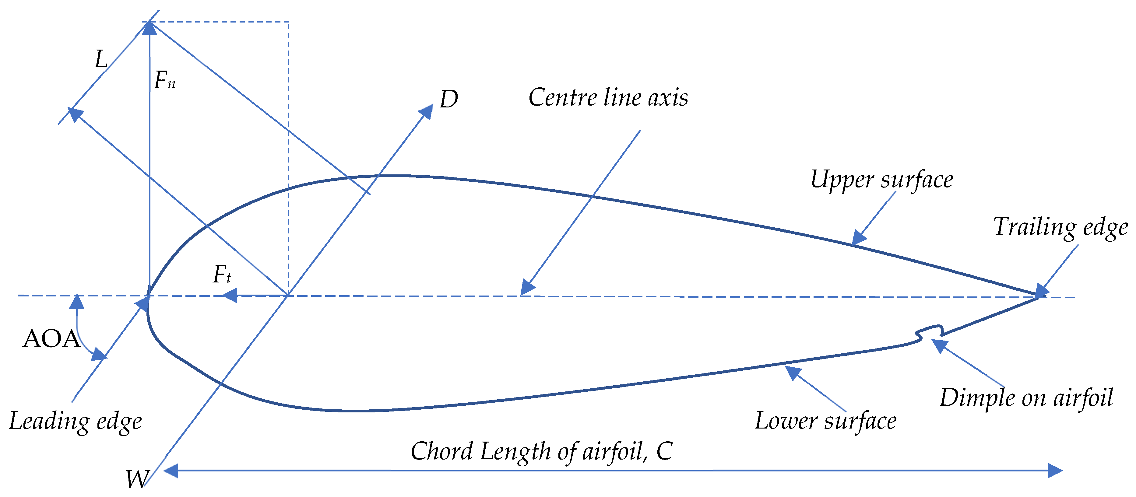
Funding

This research received no external funding. However, the article processing charges (APC) for this article were funded by author 2: C.V.A., with support from MDPI’s Inventions.

Institutional Review Board Statement

Not applicable.

Informed Consent Statement

Not applicable.

Data Availability Statement

The data supporting the reported results cannot be shared at this time, as it is being used in producing more publications on this research.

Acknowledgments

The authors wish to acknowledge the support of Lancaster University Engineering Department, Lancaster, UK for support in performing this research work. The authors also acknowledge the suggestions and support of Armin Kanani of Lancaster University in the CFD geometry designs. The authors appreciate the academic licenses provided by Autodesk and SimScale, which were used in this study. The authors also acknowledge the support of SimScale to use its online platform in this investigation.

Conflicts of Interest

The authors declare no conflict of interest. The funders had no role in the design of the study; in the collection, analyses, or interpretation of data; in the writing of the manuscript, or in the decision to publish the results. The authors declare that they have no known competing financial interests or personal relationships that could have appeared to influence the work reported in this paper.

References

  1. Collins. Definition of ‘Aeroplane’. 2019. Available online: https://www.collinsdictionary.com/dictionary/english/aeroplane (accessed on 20 August 2019).
  2. BBC. Amazon to Deliver by Drone ‘within Months’. 2019. Available online: www.bbc.com/news/technology-48536319 (accessed on 11 July 2020).
  3. CNN. Watch First-Ever Drone Delivery of ORGAN for Transplant. 2019. Available online: https://www.cnn.com/videos/health/2019/04/29/transplant-drone-delivery (accessed on 11 July 2020).
  4. Scalea, J.R.; Restaino, S.; Scassero, M.; Blankenship, G.; Bartlett, S.T.; Wereley, N. An Initial Investigation of Unmanned Aircraft Systems (UAS) and Real-Time Organ Status Measurement for Transporting Human Organs. IEEE J. Transl. Eng. Health Med. 2018, 6, Art no. 4000107. [Google Scholar] [CrossRef] [PubMed]
  5. Heyman, C. The British Army: A Pocket Guide 2012–2013; Pen and Sword: Barnsley, UK, 2011. [Google Scholar]
  6. Reckzeh, D. Aerodynamic design of the high-lift-wing for a Megaliner aircraft. Aerosp. Sci. Technol. 2003, 7, 107–119. [Google Scholar] [CrossRef]
  7. Antonov Airlines. AN-225 MRIYA. Available online: https://www.antonov-airlines.com/ (accessed on 12 December 2019).
  8. US Air Force. F-16 Fighting Falcon. 2015. Available online: https://www.af.mil/About-Us/Fact-Sheets/Display/Article/104505/f-16-fighting-falcon/ (accessed on 20 December 2019).
  9. Newman, D.G. Flying Fast Jets: Human Factors and Performance Limitations; CRC Press: Boca Raton, FL, USA, 2017. [Google Scholar]
  10. Bishop, E. The Mosquito: The Wooden Wonder; Smithsonian Institution Press: Washington, DC, USA, 1990. [Google Scholar]
  11. Choi, J.; Jeon, W.P.; Choi, H. Mechanism of drag reduction by dimples on a sphere. Phys. Fluids 2006, 18, 041702. [Google Scholar] [CrossRef] [Green Version]
  12. Davies, J.M. The aerodynamics of golf balls. J. Appl. Phys. 1949, 20, 821–828. [Google Scholar] [CrossRef]
  13. Alam, F.; Steiner, T.; Chowdhury, H.; Moria, H.; Khan, I.; Aldawi, F.; Subic, A. A study of golf ball aerodynamic drag. Procedia Eng. 2011, 13, 226–231. [Google Scholar] [CrossRef] [Green Version]
  14. Arunkumar, A.; Gowthaman, T.S.; Muthuraj, R.; Vinothkumar, S.; Balaji, K. Numerical Investigation over Dimpled Wings of an Aircraft. Int. J. Res. Appl. Sci. Eng. Technol. 2017, 5, 2017. Available online: http://www.ijraset.com/fileserve.php?FID=7034 (accessed on 14 February 2022). [CrossRef]
  15. Soh, Z.P.; Al-Obaidi, A.S.M. Numerical Analysis of the Shape of Dimple on the Aerodynamic Efficiency of NACA 0012 Airfoil. In Proceedings of the 6th EURECA 2016 Conference (Paper Number 2ME25), Kuala Lumpur, Malaysia, 6–7 December 2016; pp. 746–759. [Google Scholar]
  16. Menter, F. Zonal two equation k-w turbulence models for aerodynamics flows. In Proceedings of the AIAA 23rd Fluid Dynamics, Plasmadynamics, and Lasers Conference, Orlando, FL, USA, 6–9 July 1993. [Google Scholar] [CrossRef]
  17. Menter, F.R. Two-Equation Eddy-Viscosity Turbulence Models for Engineering Applications. AIAA J. 1994, 32, 1598–1605. [Google Scholar] [CrossRef] [Green Version]
  18. Klaib, A. The Aerodynamic Effects of Dimples on the Fuselage of an Aircraft; Report; California State Polytechnic University: Pomona, CA, USA, 2017; Available online: https://scholarworks.calstate.edu/downloads/wd375z50v?locale=en (accessed on 20 February 2022).
  19. Livya, E.; Anitha, G.; Valli, P. Aerodynamic Analysis of Dimple Effect on Aircraft Wing. Int. J. Aerosp. Mech. Eng. 2015, 9, 350–353. [Google Scholar] [CrossRef]
  20. Gregg, J.R. Design and Experimental Testing of Small-Scale Wind Turbines. Ph.D. Thesis, Baylor University, Waco, TX, USA, 2011. [Google Scholar]
  21. Anyoji, M.; Nonomura, T.; Aono, H.; Oyama, A.; Fujii, K.; Nagai, H.; Asai, K. Computational and experimental analysis of a high-performance airfoil under low-Reynolds-number flow condition. J. Aircr. 2014, 51, 1864–1872. [Google Scholar] [CrossRef]
  22. MIT. Fluids-Lecture 3 Notes. 2016. Available online: https://web.mit.edu/16.unified/www/FALL/fluids/Lectures/f03.pdf (accessed on 12 May 2020).
  23. Autodesk, S.S.T. K-Omega Turbulence Models. 2019. Available online: https://knowledge.autodesk.com/support/cfd/learn-explore/caas/CloudHelp/cloudhelp/2014/ENU/SimCFD/files/GUID-0F5C4828-9F91-46B6-A16A-2578D72DCFCC-htm.html (accessed on 23 March 2020).
  24. Airfoil Tools. BOEING 737 ROOT AEROFOIL (b737a-il). 2020. Available online: http://airfoiltools.com/airfoil/details?airfoil=b737a-il (accessed on 15 March 2020).
  25. Wilkerson, J.T.; Jacobson, M.Z.; Malwitz, A.; Balasubramanian, S.; Wayson, R.; Fleming, G.; Naiman, A.D.; Lele, S.K. Analysis of emission data from global commercial aviation: 2004 and 2006. Atmos. Chem. Phys. 2010, 10, 6391–6408. [Google Scholar] [CrossRef] [Green Version]
  26. Boeing. BOEING 787 DREAMLINER. 2020. Available online: https://www.boeing.com/commercial/787/ (accessed on 12 March 2020).
  27. Modern Airliners. BOEING 787 Dreamliner Specs. 2020. Available online: https://modernairliners.com/boeing-787-dreamliner/boeing-787-dreamliner-specs/ (accessed on 12 March 2020).
  28. Gudmundsson, S. General Aviation Aircraft Design, 1st ed.; Butterworth–Heinemann: Oxford, UK, 2013. [Google Scholar]
  29. Zhang, Y.; Ren, Q.; Zhao, Y.P. Modelling analysis of surface stress on a rectangular cantilever beam. J. Phys. D Appl. Phys. 2004, 37, 2140. [Google Scholar] [CrossRef]
  30. Králik, J. CFD Simulation of Air Flow Over an Object with Gable Roof, Revised with Y+ Approach. Trans. VŠB–Tech. Univ. Ostrav. Civ. Eng. Ser. 2016, 16, 85–94. [Google Scholar] [CrossRef] [Green Version]
  31. Babinksy, H. How do wings work? Phys. Educ. 2003, 38, 497–503. Available online: http://www3.eng.cam.ac.uk/outreach/Project-resources/Wind-turbine/howwingswork.pdf (accessed on 11 February 2022).
  32. Gemba, K. Measurement of Boundary Layer on a Flat Plate; Experimental Report; California State University: Long Beach, CA, USA, 2007. [Google Scholar]
  33. Selig, M.S.; Maughmer, M.D.; Somers, D.M. Natural-laminar-flow airfoil for general-aviation applications. J. Aircr. 1995, 32, 710–715. [Google Scholar] [CrossRef] [Green Version]
  34. Evans, P. Properties of Air at Atmospheric Pressure. 2015. Available online: https://theengineeringmindset.com/properties-of-air-at-atmospheric-pressure/ (accessed on 2 February 2020).
  35. Hassan, G.; Hassan, A.; Youssef, M.E. Numerical Investigation of Medium Range Re Number Aerodynamics Characteristics for NACA0018 Airfoil. CFD Lett. 2015, 6, 175–187. Available online: https://www.researchgate.net/publication/280087418_Numerical_Investigation_of_Medium_Range_Re_Number_Aerodynamics_Characteristics_for_NACA0018_Airfoil (accessed on 20 February 2022).
  36. Ariff, M.; Salim, S.M.; Cheah, S.C. Wall y+ approach for dealing with turbulent flow over a surface mounted cube: Part 2—High Reynolds number. In Proceedings of the Seventh International Conference on CFD in the Minerals and Process Industries CSIRO, Melbourne, Australia, 9–11 December 2009; pp. 9–11. Available online: https://www.researchgate.net/publication/209105898_Wall_y_Approach_for_Dealing_with_Turbulent_Flows_over_a_Surface_Mounted_Cube_Part_2_-_High_Reynolds_Number (accessed on 14 February 2022).
  37. Winslow, J.; Otsuka, H.; Govindarajan, B.; Chopra, I. Basic Understanding of Airfoil Characteristics at Low Reynolds Numbers (104–105). J. Aircr. 2018, 55, 1050–1061. [Google Scholar] [CrossRef]
  38. TecPlot. CFD Visualisation & Analysis Tool. 2016. Available online: https://www.tecplot.com/products/tecplot-360/ (accessed on 19 February 2022).
Figure 1. Illustration depicting the constituent forces acting on dimpled aerofoils, including its AOA.
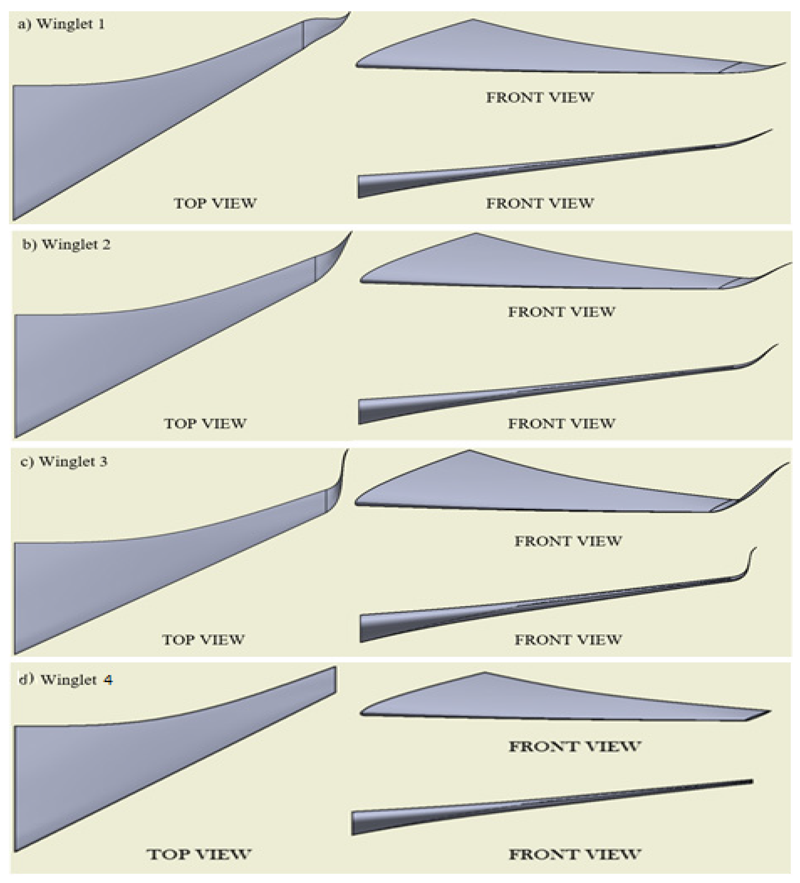
Inventions 07 00031 g001
Figure 2. Winglet designs (a) 20° cant angle, extending 4 m from main wing, height of 1 m (b) 45° cant angle, extending 3 m, with a height of 2 m (c) 65° cant angle, extending 2 m, with a height of 3 m (d) 0° for the Boeing 787-9 Dreamliner wing.
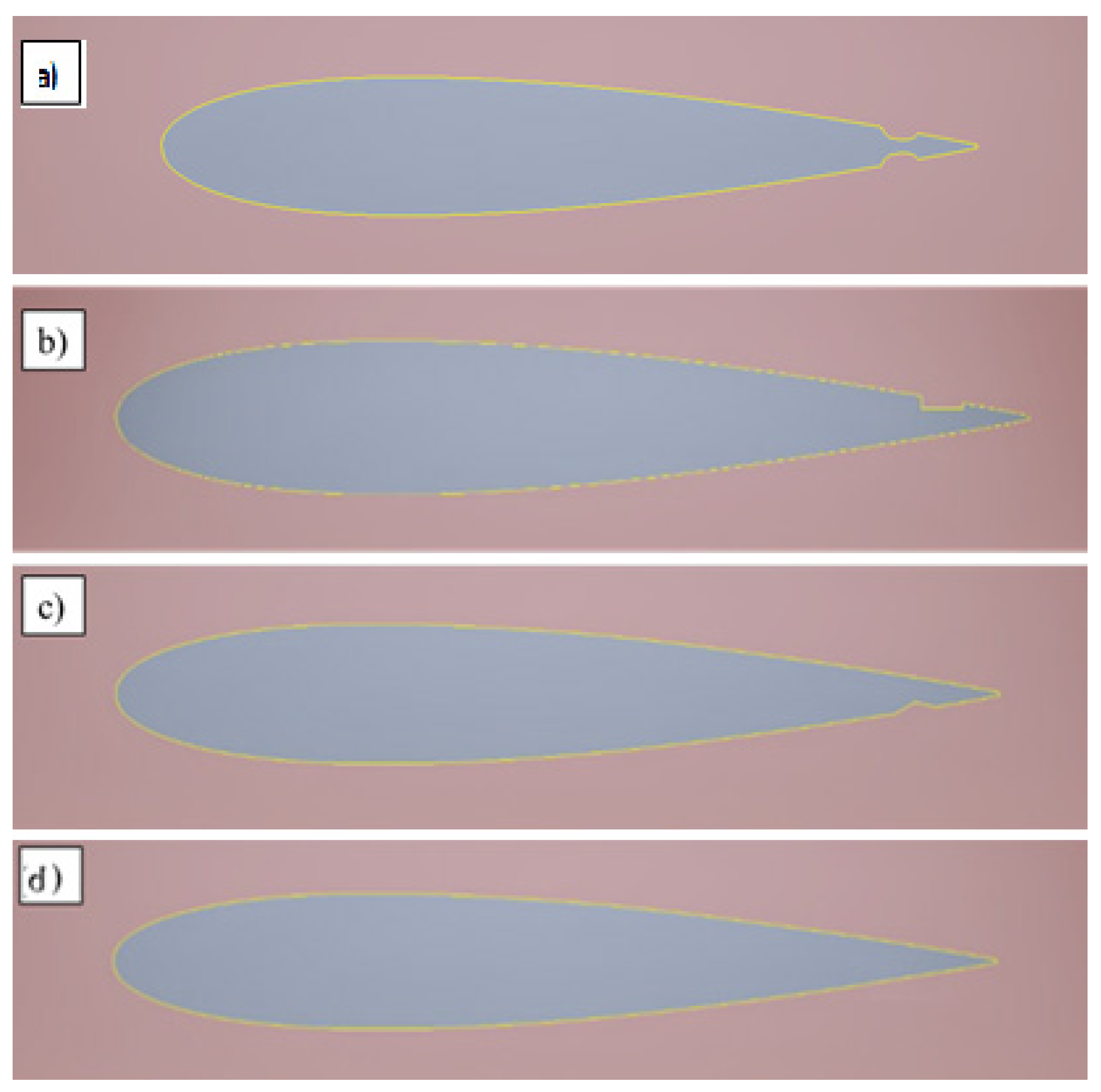
Inventions 07 00031 g002
Figure 3. Geometry designs for different model, showing (a) elliptical dimples placed on the top and bottom of the aerofoil, (b) square dimple placed on top of the aerofoil, (c) triangular dimple underneath the aerofoil, and (d) no dimple aerofoil.
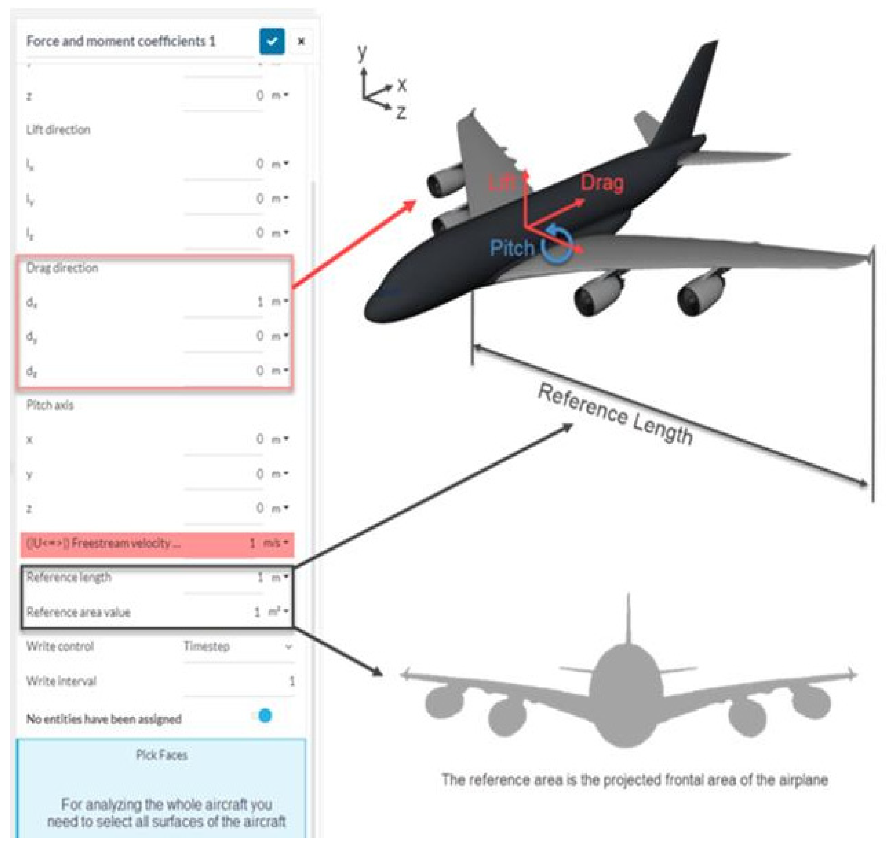
Inventions 07 00031 g003
Figure 4. The reference area of the aircraft wings in SimScale platform.
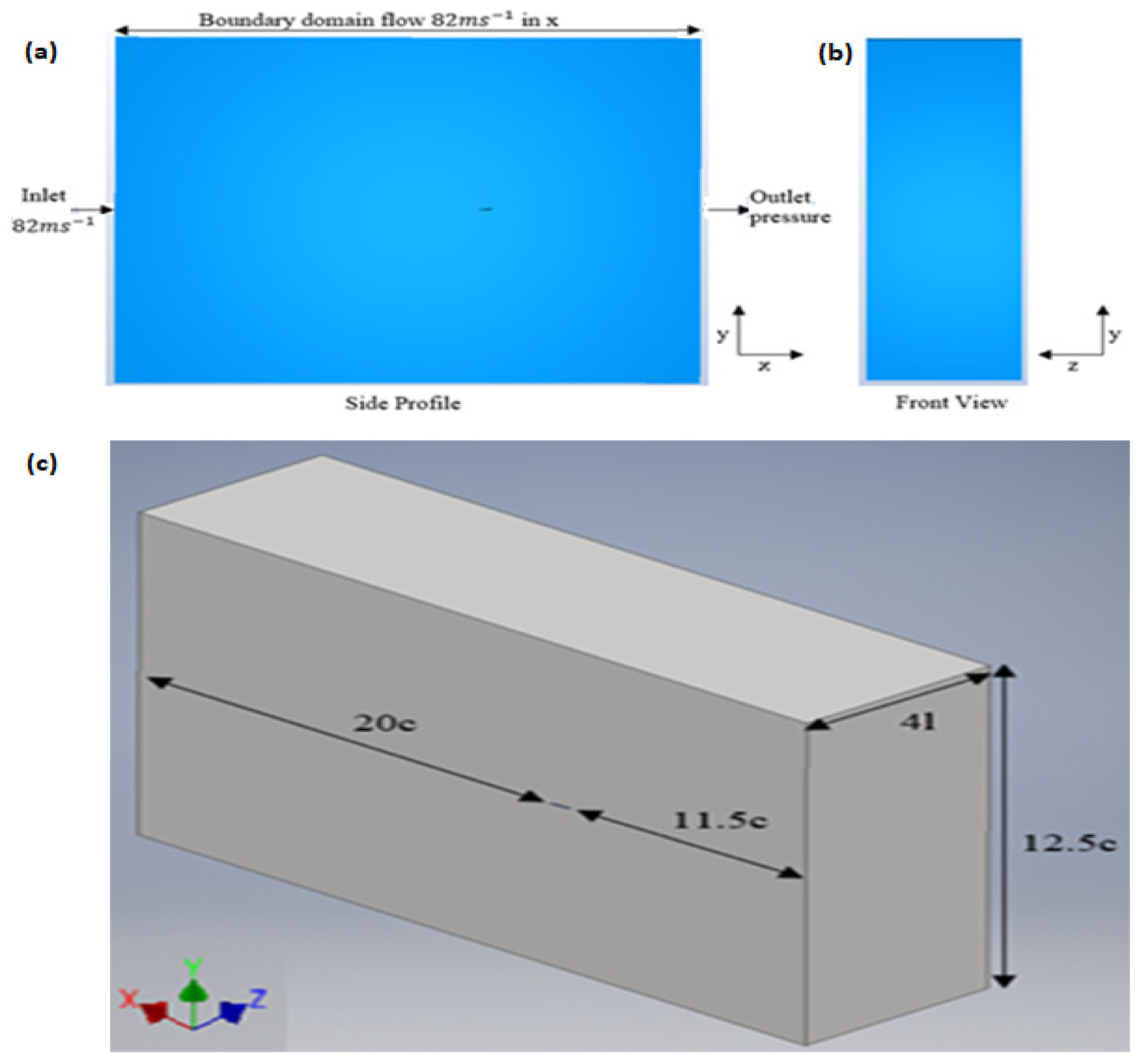
Inventions 07 00031 g004
Figure 5. Boundary domain flow of the enclosure for the winglet in 3D, showing (a) side, (b) front, and (c) isometric views.
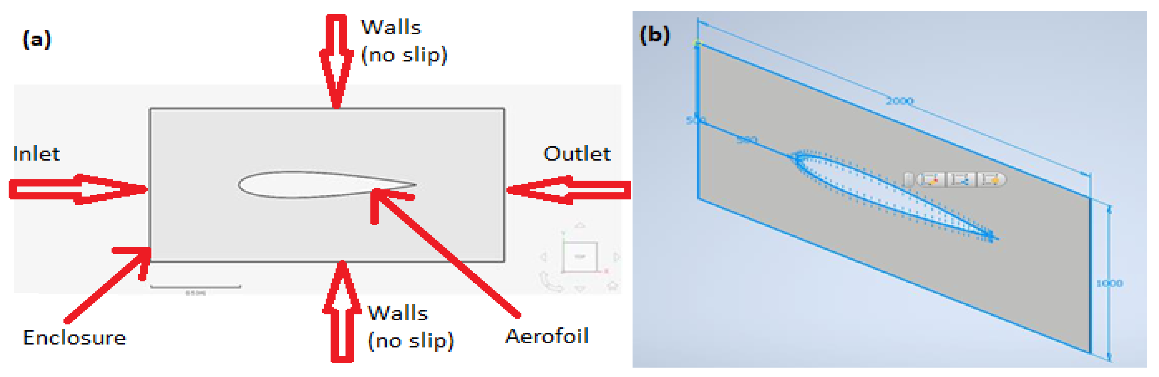
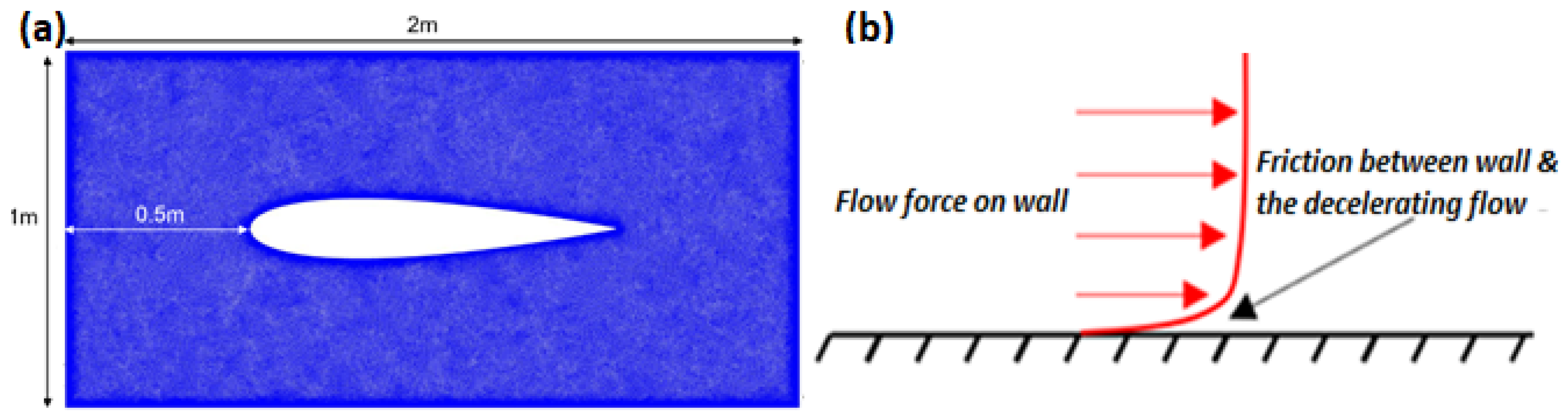
Inventions 07 00031 g005
Figure 6. Flow Domain of the aerofoil in 2D, showing (a) boundary conditions, and (b) enclosure dimensions.
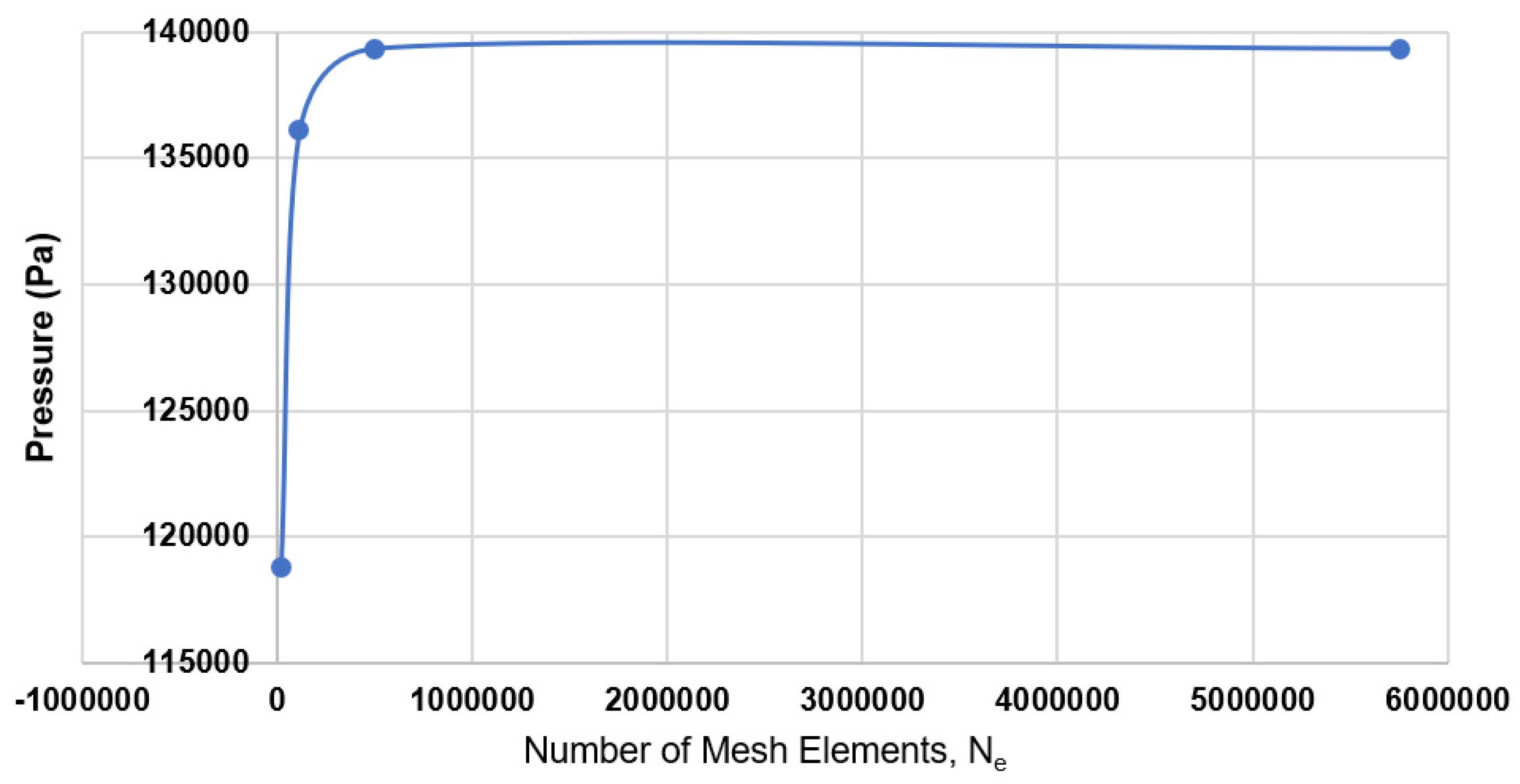
Inventions 07 00031 g006
Figure 7. Mesh convergence study showing relationship between pressure and number of elements in 3D.
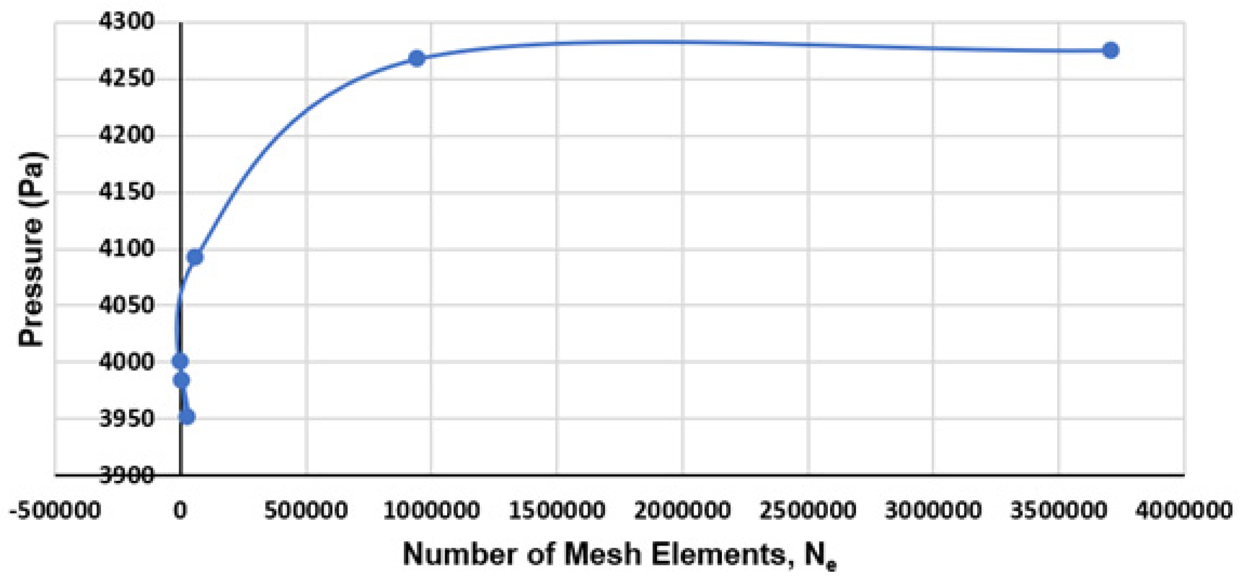
Inventions 07 00031 g007
Figure 8. Mesh convergence study for stabilization of pressure as number of elements increases in 2D.
Inventions 07 00031 g008
Figure 9. The effect of pressure on force exerted on the leading edge of wing.
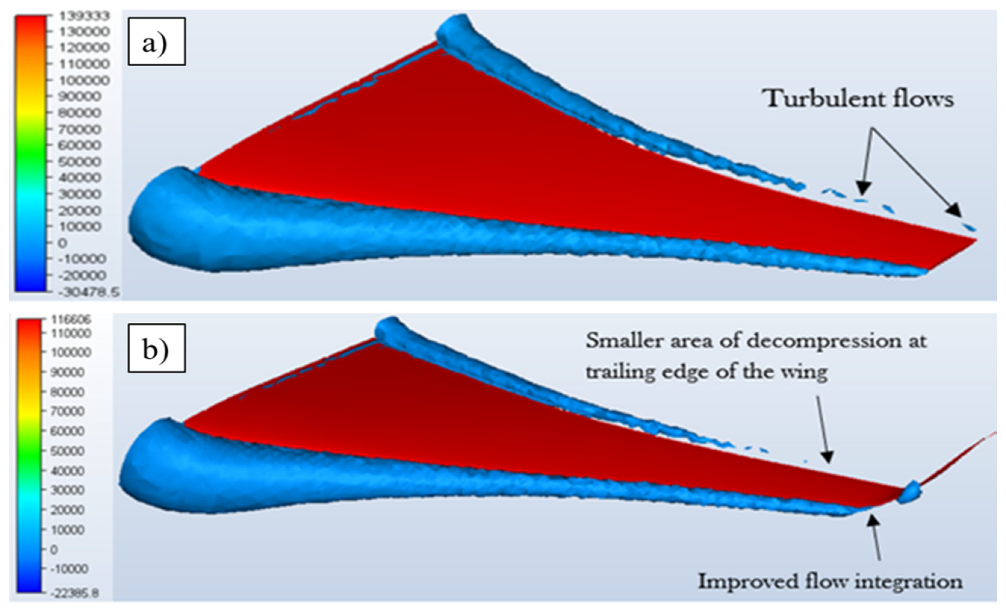
Inventions 07 00031 g009
Figure 10. Pressure plot on (a) unmodified wing and (b) modified wing.
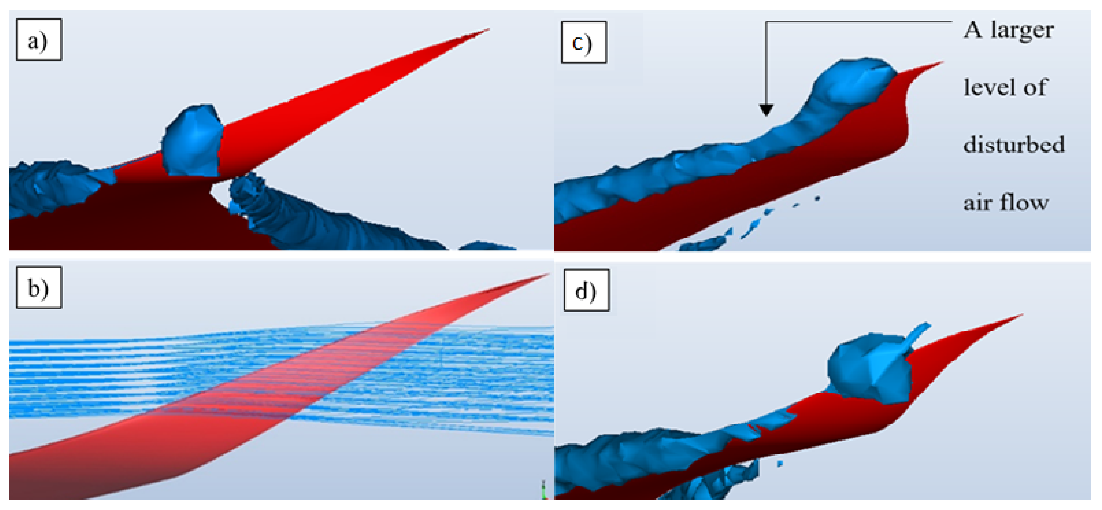
Inventions 07 00031 g010
Figure 11. The flow streamline, showing (a) underside of aerofoil with attached winglet, (b) flow phenomenon over winglet, (c) disturbed air flow on winglet 1, and (d) disturbed airflow on winglet 2.
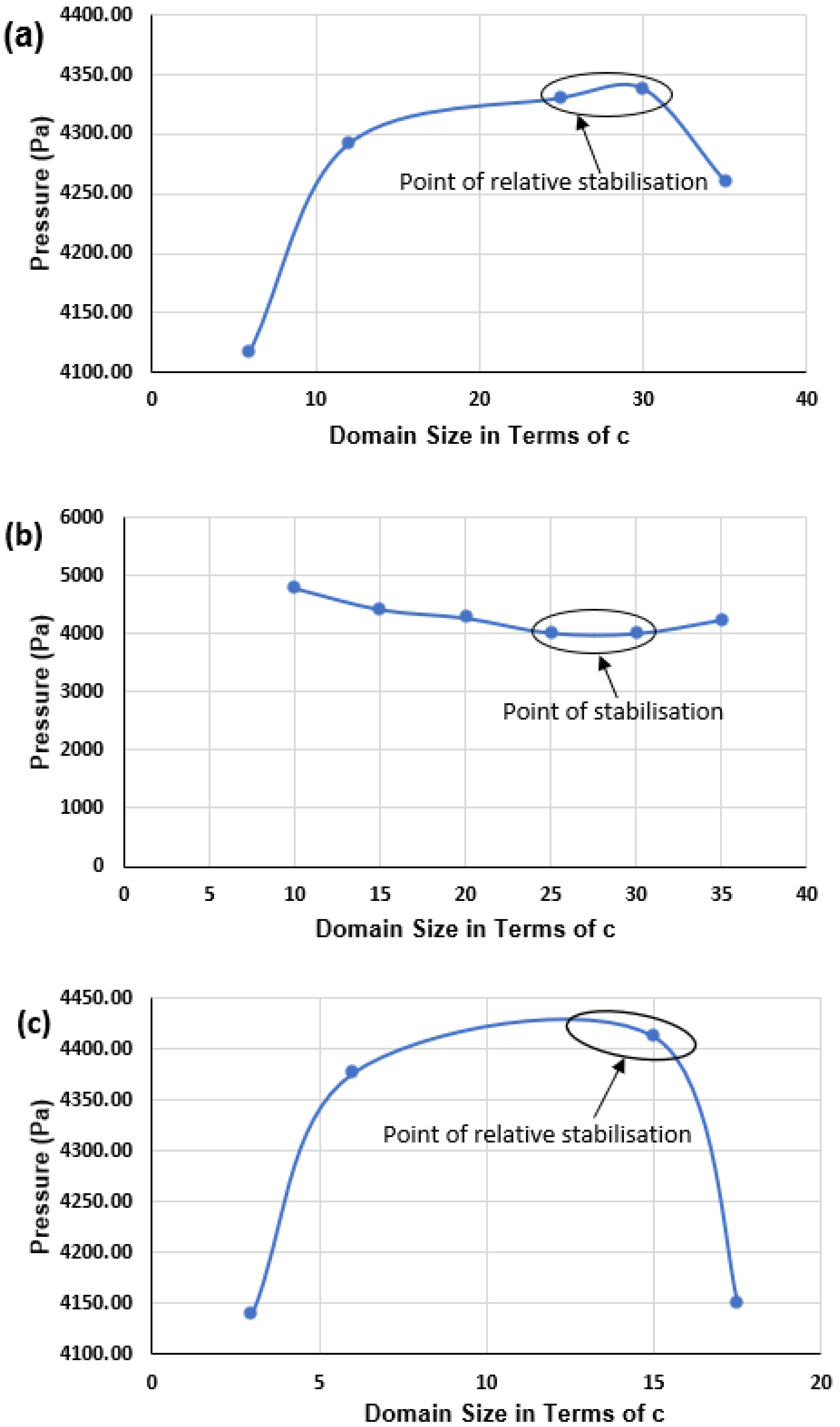
Inventions 07 00031 g011
Figure 12. Pressure variation against distance for the dimple study, showing (a) y-direction stabilization point, (b) front-aerofoil stabilization points, and (c) behind-aerofoil stabilization points.
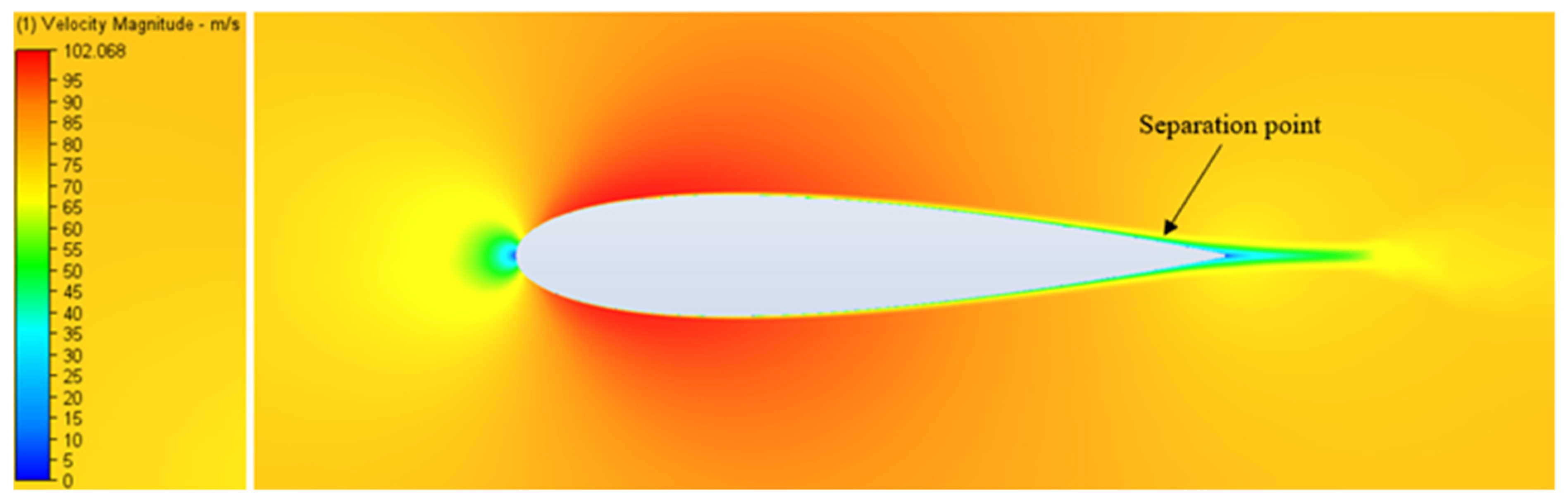
Inventions 07 00031 g012
Figure 13. NACA 0017 aerofoil acting at 0° AOA showing Separation point over.
Inventions 07 00031 g013
Figure 14. Creation of the (a) boundary domain mesh and (b) boundary layer showing friction region.
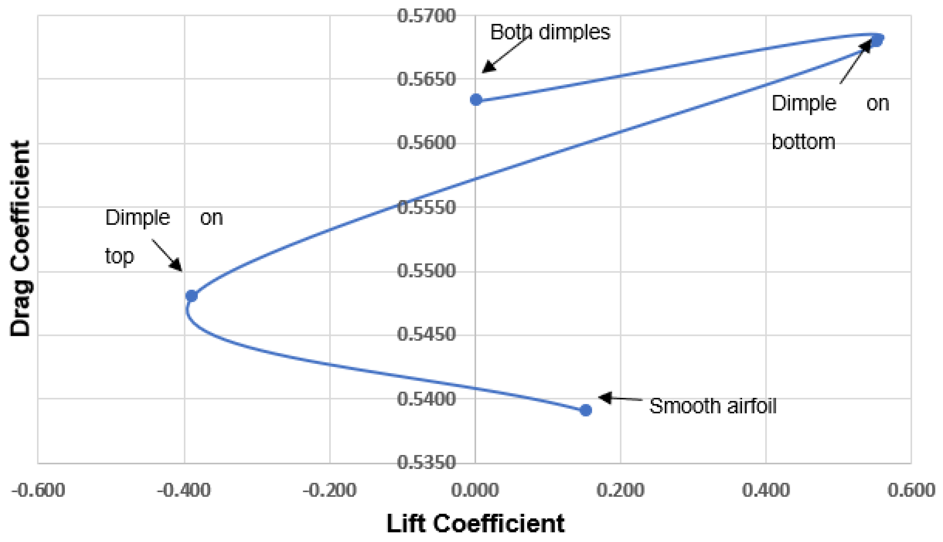
Inventions 07 00031 g014
Figure 15. The relationship between lift and drag coefficients on an aerofoil with an ellipse-shaped dimple.
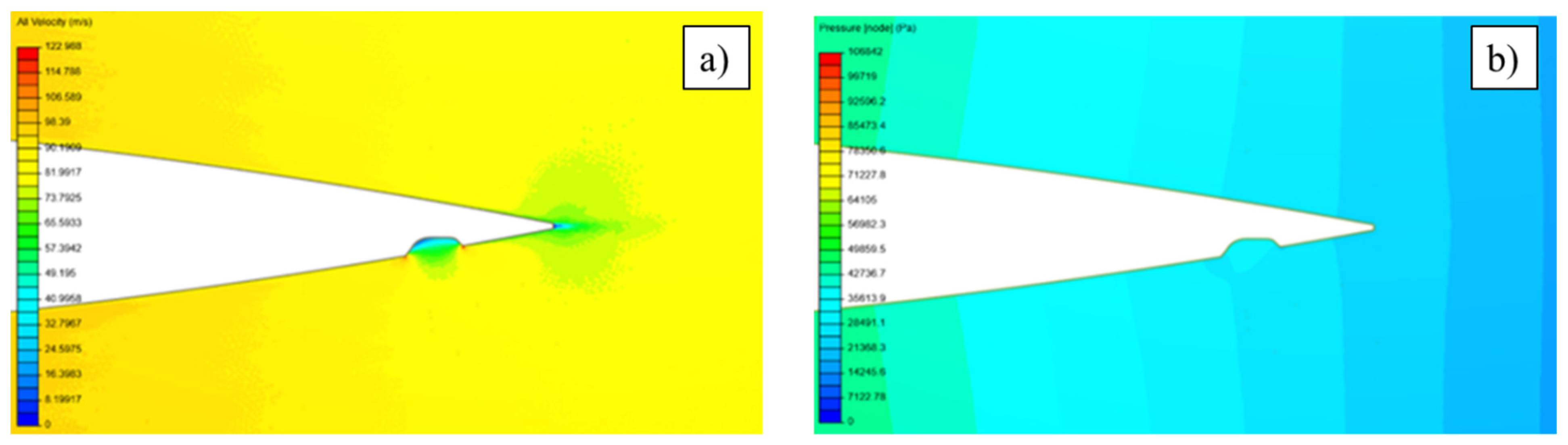
Inventions 07 00031 g015
Figure 16. Profiles of total (a) velocity and (b) pressure over dimples aerofoil, SimScale simulation.
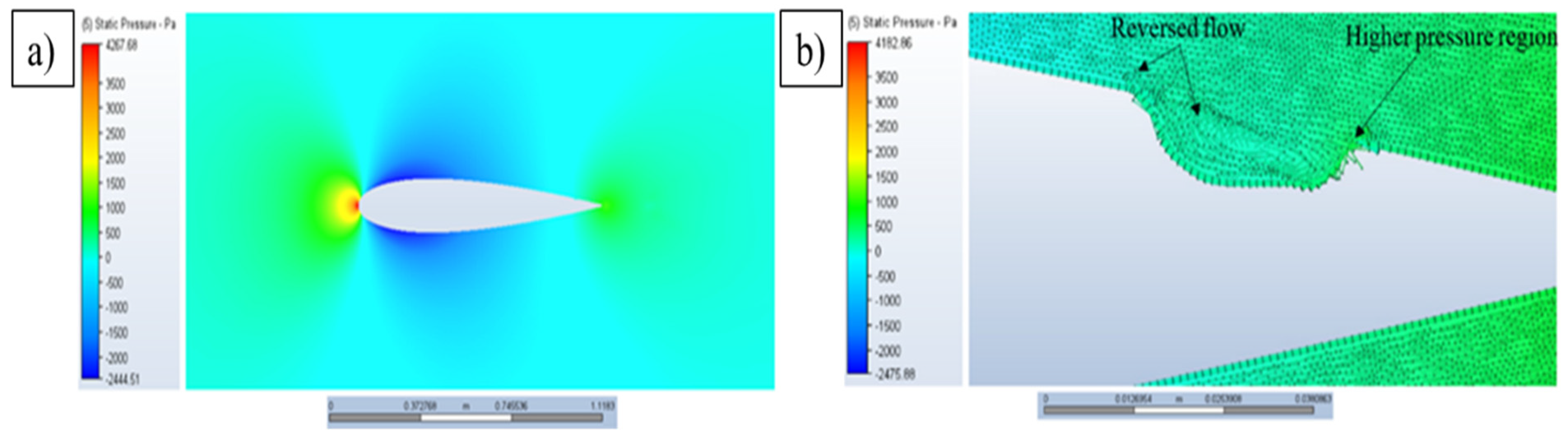
Inventions 07 00031 g016
Figure 17. (a) Pressure gradient and (b) flow disturbance over unmodified 2D aerofoil.
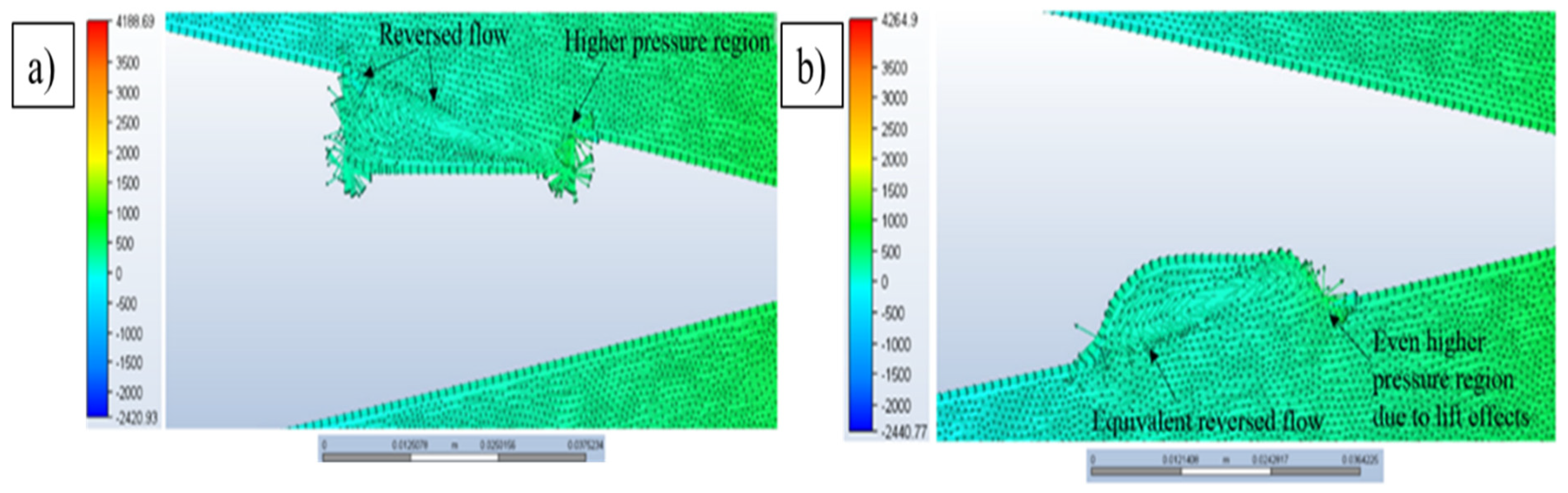
Inventions 07 00031 g017
Figure 18. Exploded views showing (a) visualisation of the increased levels of drag induced by a square dimple and (b) flow phenomenon when a dimple is placed underneath the aerofoil.
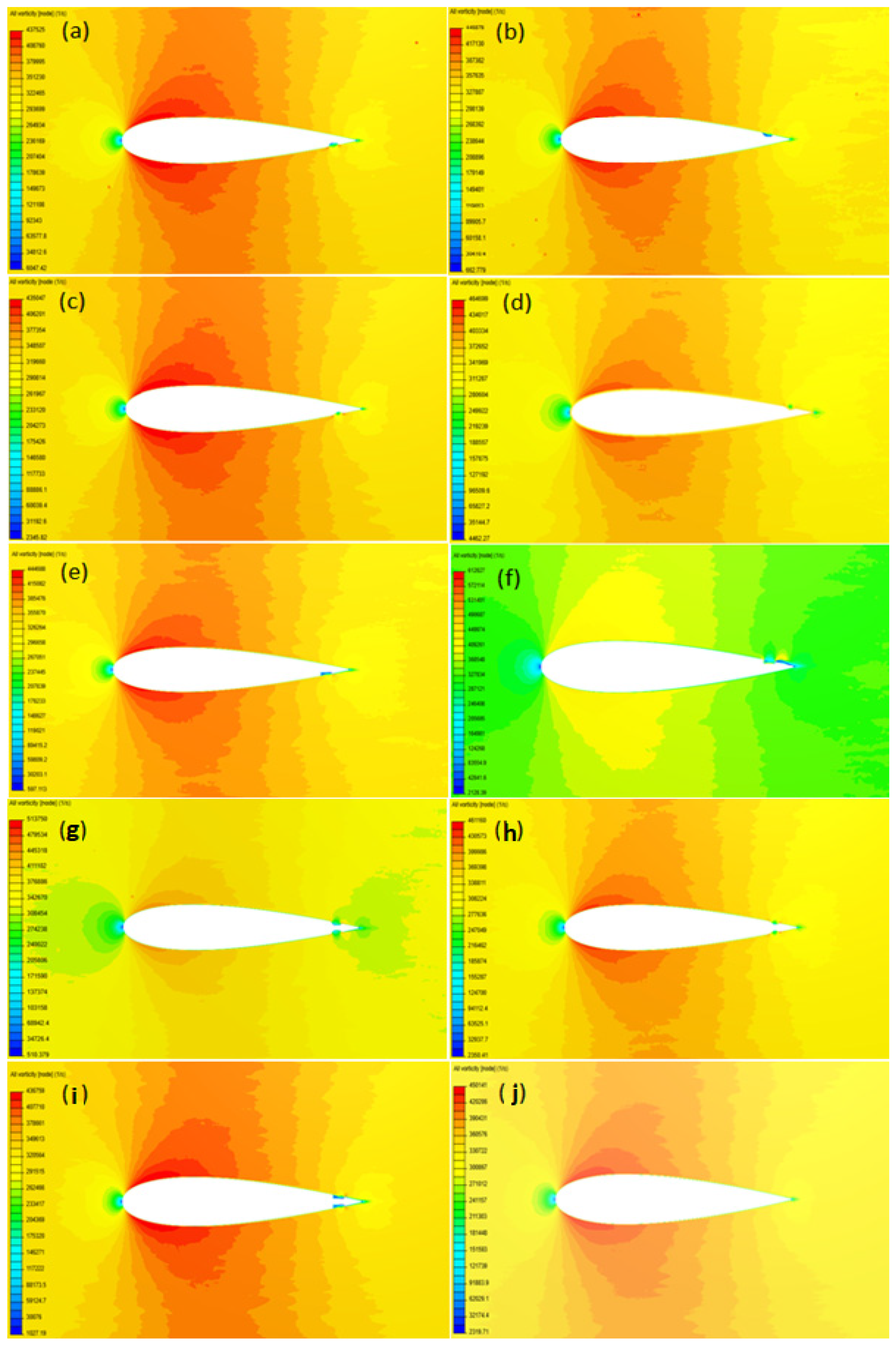
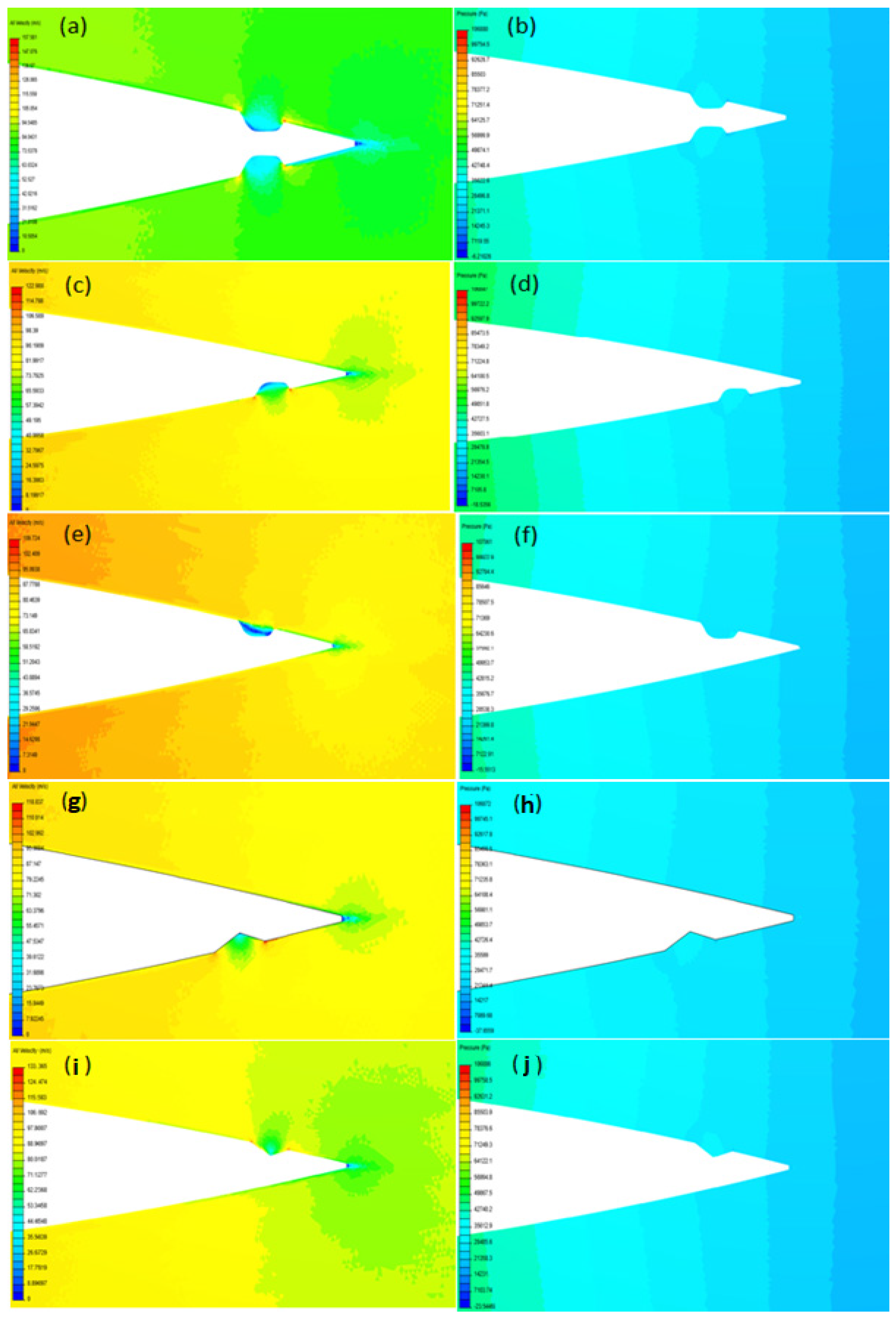
Inventions 07 00031 g018
Figure 19. Vorticity profile on (a) round bottom dimple, (b) round top dimple, (c) triangle bottom dimple, (d) triangle top dimple, (e) square bottom dimple, (f) square top dimple, (g) round dimple both ends, (h) triangle dimple both ends, (i) square dimple both ends, and (j) no dimple aerofoil design.
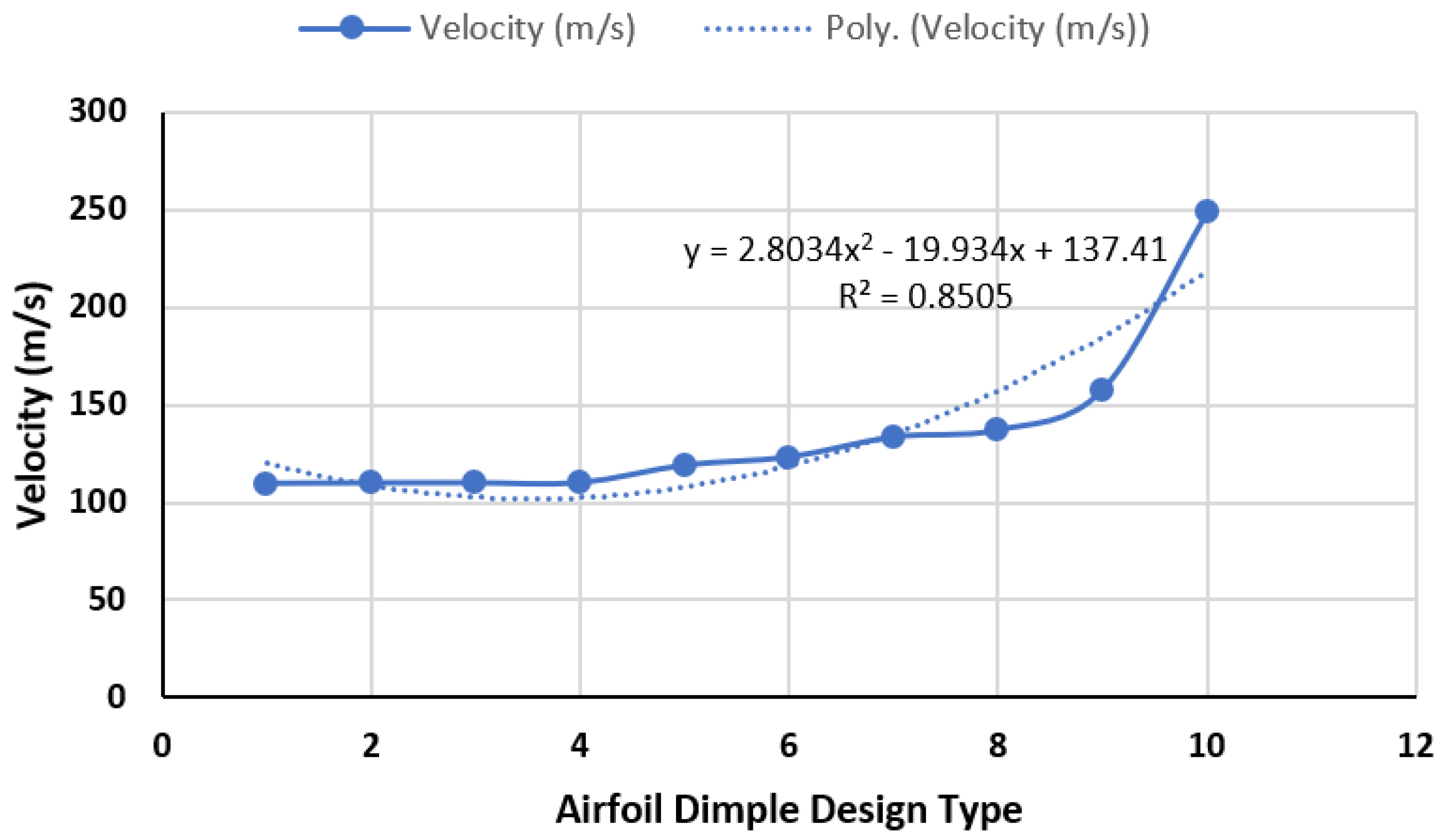
Inventions 07 00031 g019
Figure 20. The velocity plot for the 10 dimple aerofoil designs.
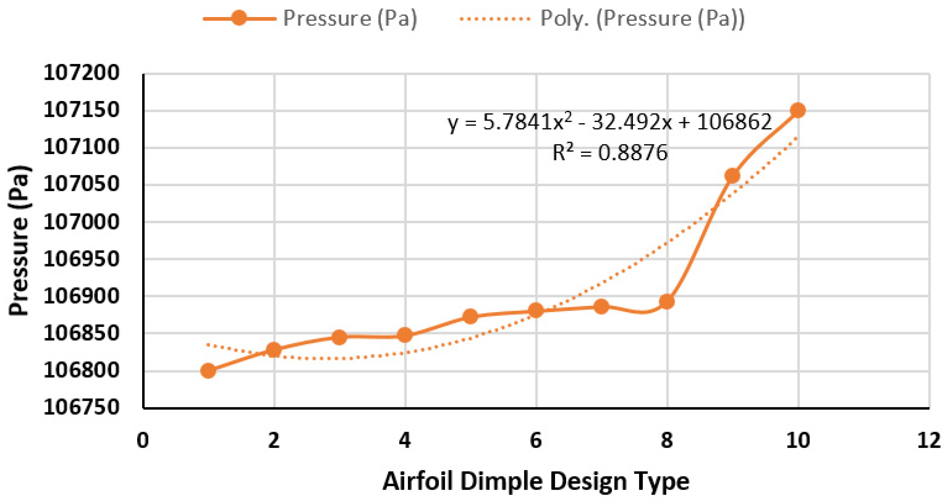
Inventions 07 00031 g020
Figure 21. The pressure plot for the 10 dimple aerofoil designs.
Inventions 07 00031 g021
Figure 22. Exploded view showing (a) velocity profile on round dimple on both ends, (b) pressure profile on round dimple on both ends, (c) velocity profile on round bottom dimple, (d) pressure profile on round bottom dimple, (e) velocity profile on round top dimple, (f) pressure profile on round top dimple, (g) velocity profile on triangle bottom dimple, (h) pressure profile on triangle bottom dimple, (i) velocity profile on triangle top dimple, and (j) pressure profile on triangle top dimple.
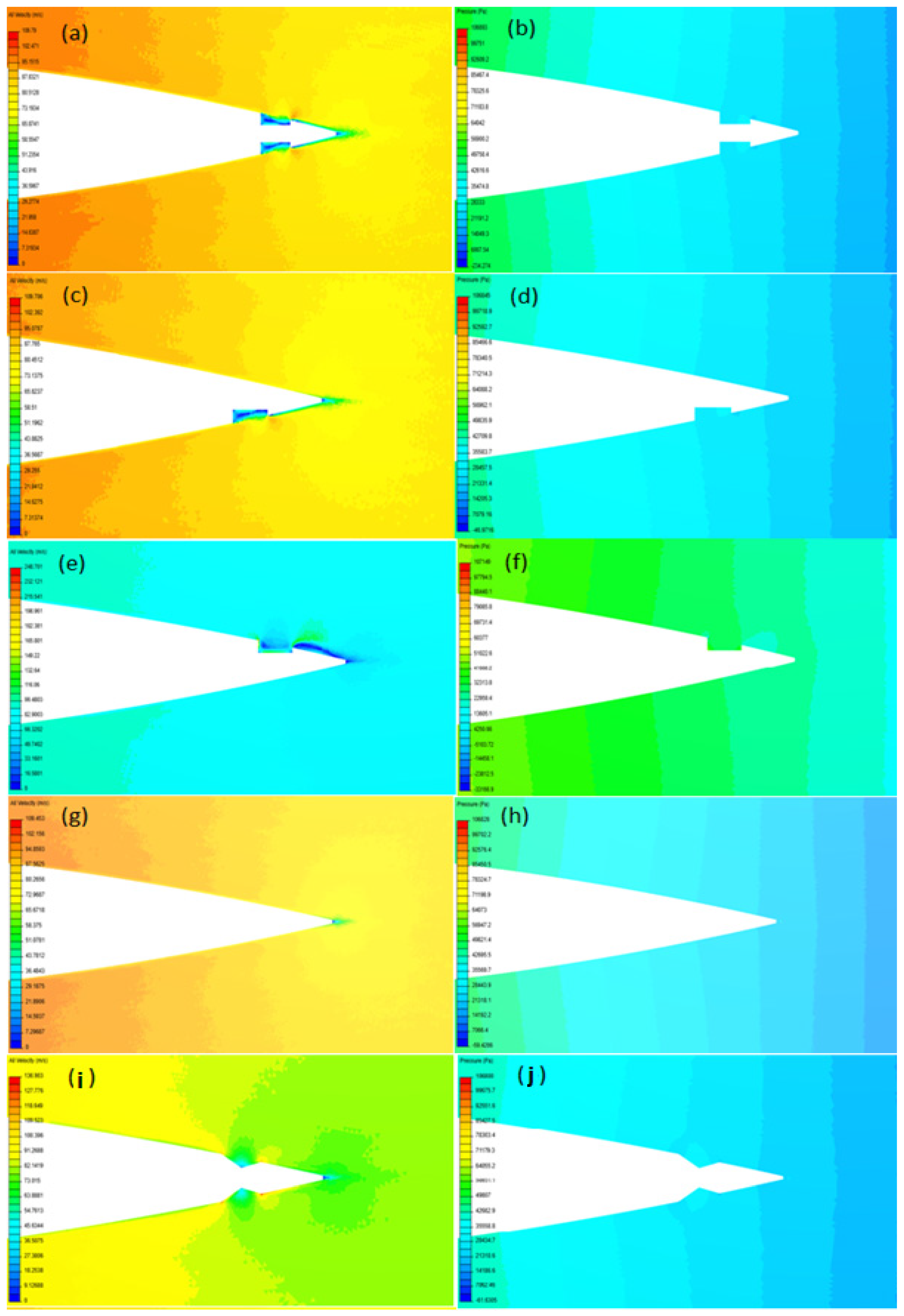
Inventions 07 00031 g022
Figure 23. Exploded view showing (a) velocity profile on square dimple on both ends, (b) pressure profile on square dimple on both ends, (c) velocity profile on square bottom dimple, (d) pressure profile on square bottom dimple, (e) velocity profile on square top dimple, (f) pressure profile on square top dimple, (g) velocity profile on aerofoil with no dimple, (h) pressure profile on aerofoil with no dimple, (i) velocity profile on triangle dimple on both ends, and (j) pressure profile on triangle dimple on both ends.
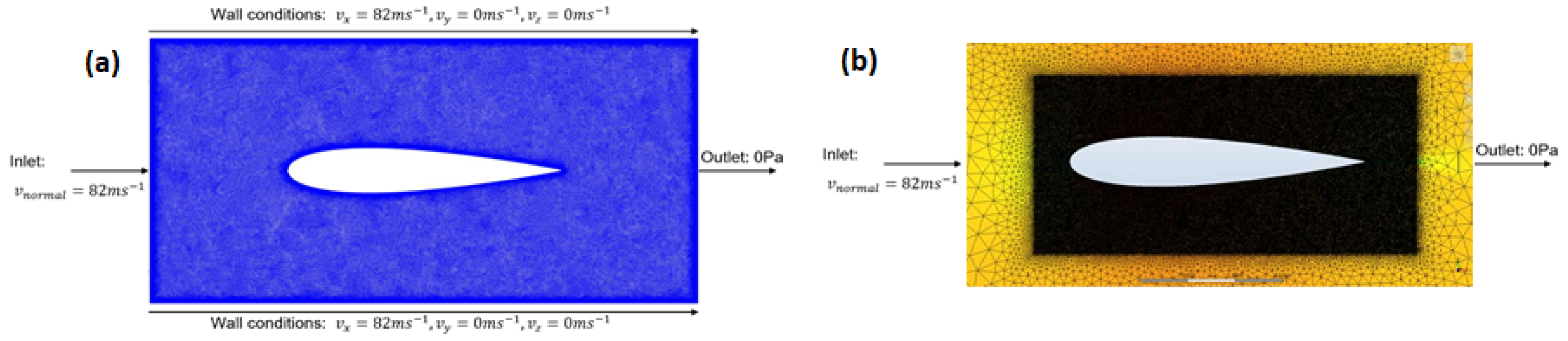
Inventions 07 00031 g023
Figure 24. Dimple study boundary domain, showing (a) wall conditions, and (b) refined mesh model.
Inventions 07 00031 g024
Table 1. Details of the Freighter aircraft.
ParameterValue
Total wingspan60 m
Root chord length13.5 m
Speed range1350 km
Take-off weight254,011 kg
Take-off speed chosen82 m/s
Table 2. Parameters for the enclosure for the aerofoil dimple designs in 2D.
ParameterValue (mm)
Leading Edge to Front Boundary15,000
Trailing Edge to Rear Boundary30,000
Total Boundary Length46,000
Leading Edge to Horizontal Boundary15,000
Total Boundary Height30,000
Aerofoil Length1000
Maximum Aerofoil Height170
Dimple Length for ELLIPSE Design46.835
Max. Dimple Depression Depth ELLIPSE11.94
Dimple Length for SQUARE Design46.835
Max. Dimple Depression Depth SQUARE13.962
Dimple Length for TRIANGLE Design46.835
Max. Dimple Depression Depth TRIANGLE9.879
Table 3. Parameters for the Initial Boundary Conditions.
ParametersValues
Inlet Velocity, ( v t a k e - o f f )82 m/s
Air Temperature, T19.85 °C
Density of Air, ρ a i r 1.225 Kg/m3
Viscosity of Air, μ a i r 1.81 × 10⁻⁵ Kg/m
Gas Constant287.05 m2/s2–k
Compressibility Constant1.4
Inlet Pressure (Gauge)0 Pa
Outlet Pressure (Gauge)0 Pa
Mesh Size1 mm sub-domain (and auto)
Mesh TypeTetrahedral
Flow TypeIncompressible (steady state)
Fluid TypeInviscid
Turbulent ModelK-omega SST
Side WallsSlip/Symmetry
Reynolds Number (2D)5.55 × 10⁶
Reynolds Number (3D)76.314 × 10⁶
Table 4. Mesh Refinement Regions for the 2D Model.
Region TypeBox Region
X Offset0.5286 m
Y Offset−0.0096 m
Z Offset0 m
X Length1.2854 m
Y Length0.5963 m
Z Length0 m
Table 5. Results of the Mesh Independence Study in 3D Winglet Analysis.
Mesh SchemeElement Size (mm)Number of ElementsTime (Minutes)Pressure (Pa)
Auto-sized252019,9537118,766.00
Refined wing edges500116,29440136,106.00
Refined wing edges with regions90505,390210139,333.00
Wing edges and regions are both refined605,761,7651274139,331.00
Table 6. Effect of Mesh Size on Pressure in the 2D Dimple Effect Analysis.
Mesh SchemeMesh Size (mm)ElementsTime (Minutes)Pressure (Pa)
Auto-sized20237334000.28
Refined wing edges57354123983.80
Refined wing edges230,604273951.44
Refined wing edges160,520444091.87
Refined wing edges with regions1946,10111794267.88
Refined wing edges with regions0.53,711,71357,4544275.42
Table 7. Pressure comparison showing percentage difference between each winglet design and a conventional wing.
IDFinal Pressure (Pa)Percentage DifferenceForce (N) × 106
No-winglet139,333.00-48.39
Winglet-1123,199.0011.5744.36
Winglet-2119,803.0014.0142.90
Winglet-3116,606.0016.3141.61
Table 8. Pressure fluctuation as boundary domain changes size.
Boundary Domain in Terms of cElementsPressure Value (Pa)
Y value
626424117.41
1226904291.67
2524554330.38
3027804337.83
3527144259.73
X value in front of aerofoil
326764139.25
628164376.91
1527774412.88
17.528474150.67
X value behind aerofoil
1027514777.21
1527774412.88
2028694267.74
2529394008.67
3023734000.28
3525764236.08
Table 9. The pressure and velocity distribution for the 10 dimple designs.
Pressure PlotVelocity PlotGrouped Plot
DescriptorsPressure (Pa)DescriptorsVelocity (m/s)DescriptorsVelocity (m/s)Pressure (Pa)
Triangle Dimple Both106,800No Dimple109.453Round Dimple Both157.581106,880
No Dimple106,828Square Dimple Bottom109.706Round Dimple Bottom122.988106,847
Square Dimple Bottom106,845Round Dimple Top109.724Round Dimple Top109.724107,061
Round Dimple Bottom106,847Square Dimple Both109.79Triangle Dimple Both136.903106,800
Triangle Dimple Bottom106,872Triangle Dimple Bottom118.837Triangle Dimple Bottom118.837106,872
Round Dimple Both106,880Round Dimple Bottom122.988Triangle Dimple Top133.365106,886
Triangle Dimple Top106,886Triangle Dimple Top133.365Square Dimple Both109.79106,893
Square Dimple Both106,893Triangle Dimple Both136.903Square Dimple Bottom109.706106,845
Round Dimple Top107,061Round Dimple Both157.581Square Dimple Top248.701107149
Square Dimple Top107,149Square Dimple Top248.701No Dimple109.453106,828
Table 10. Results of a dimpled wing in comparison to a smooth one.
Dimple TypeDesign Case Reference PointPressure (Pa)LiftDragLift CoefficientDrag CoefficientPercentage Difference (P.D) of This Model Compared to a Conventional AerofoilEfficiency
Lift P.D.Drag P.D.
No Dimple-4267.8819.48668.3550.1540.5390--0.2850723
EllipseTop4182.86−49.58169.810−0.3890.5480−254.4442.1290−0.710229
Bottom4264.9070.45872.2890.5540.5679261.5805.75650.9746588
Both4192.920.36371.9940.0030.5633−0.7325.32430.0050412
SquareTop4188.69−31.97571.785−0.2500.5609−164.0905.0185−0.44542
Bottom4265.6460.06971.9260.4690.5620208.2665.22530.8351424
Both4174.829.54373.1200.0740.5662−51.0246.97200.1305168
TriangleTop4190.9−29.11070.967−0.2290.5586−149.3913.8214−0.410197
Bottom4265.2865.82771.9210.5180.5661237.8155.21710.9152678
Both4275.2926.73273.0030.2100.573537.1886.80090.3661807
Table 11. Results from the SimScale verification study.
Dimple TypeDesign Case Reference PointLift CoefficientDrag CoefficientPercentage Difference (P.D.) of This Model Compared to a Conventional Aerofoil
Lift P.D.Drag P.D.
No Dimple-0.0010313.3150--
EllipseTop−0.0007113.3212−168.5470.1282
Bottom0.0040913.3196296.3160.1399
Both0.0027313.3455164.9540.0541
SquareTop−0.0011313.4501−109.7590.8384
Bottom0.0034313.5110232.3681.4720
Both0.0018313.347077.7150.0658
TriangleTop−0.0013113.3143−126.939−0.1794
Bottom0.0035313.3167242.0580.1613
Both0.0001713.299816.4730.2887
Publisher’s Note: MDPI stays neutral with regard to jurisdictional claims in published maps and institutional affiliations.

