Article

Kalman Filter Adaptation to Disturbances of the Observer’s Parameters

by
Alexander A. Manin
1,
Sergey V. Sokolov
1,
Arthur I. Novikov
2,*,
Marianna V. Polyakova
1,
Dmitriy N. Demidov
2 and
Tatyana P. Novikova
2
1
Computer Science and Computer Engineering Department, Moscow Technical University of Communications and Informatics—North Caucasus Branch, 344038 Rostov-on-Don, Russia
2
Automotive Faculty, Faculty of Computer Science and Technology, Voronezh State University of Forestry and Technologies Named after G.F. Morozov, 394087 Voronezh, Russia
*
Author to whom correspondence should be addressed.
Inventions 2021, 6(4), 80; https://doi.org/10.3390/inventions6040080
Submission received: 27 September 2021 / Revised: 30 October 2021 / Accepted: 1 November 2021 / Published: 2 November 2021
(This article belongs to the Special Issue Automatic Control and System Theory and Advanced Applications)

Abstract

:
Currently, one of the most effective algorithms for state estimation of stochastic systems is a Kalman filter. This filter provides an optimal root-mean-square error in state vector estimation only when the parameters of the dynamic system and its observer are precisely known. In real conditions, the observer’s parameters are often inaccurately known; moreover, they change randomly over time. This in turn leads to the divergence of the Kalman estimation process. The problem is currently being solved in a variety of ways. They include the use of interval observers, the use of an extended Kalman filter, the introduction of an additional evaluating observer by nonlinear programming methods, robust scaling of the observer’s transmission coefficient, etc. At the same time, it should be borne in mind that, firstly, all of the above ways are focused on application in specific technical systems and complexes, and secondly, they fundamentally do not allow estimating errors in determining the parameters of the observer themselves in order to compensate them for further improving the accuracy and stability of the filtration process of the state vector. To solve this problem, this paper proposes the use of accurate observations that are irregularly received in a complex measuring system (for example, navigation) for adaptive evaluation of the observer’s true parameters of the stochastic system state vector. The development of the proposed algorithm is based on the analytical dependence of the Kalman estimate variation on the observer’s parameters disturbances obtained using the mathematical apparatus for the study of perturbed multidimensional dynamical systems. The developed algorithm for observer’s parameters adaptive estimation makes it possible to significantly increase the accuracy and stability of the stochastic estimation process as a whole in the time intervals between accurate observations, which is illustrated by the corresponding numerical example.

1. Introduction

To assess the stochastic systems state, a significant number of different algorithms and techniques [1] have been developed, among which one of the most effective is the Kalman filter [2]. However, often, a problem arises with the practical application of the Kalman filter. It is due to the fact that this filter calculates an optimal root-mean-square error (RMS-error) of state vector estimation only when both the parameters—system and state vector observer—are known exactly [3]. When operating real systems—control, communications, navigation, etc.—the parameters of both the system itself and its state vector meters, as a rule, change randomly over time. This is especially evident in imperfect dynamical systems, the interest in the study of which has only been increasing lately [4,5,6,7,8]. Such instability of the system parameters when trying to assess its current state causes the divergence of the Kalman estimation process. This disadvantage of the Kalman filter requires the development of appropriate methods to ensure, with random variations of the observer’s parameters, a given accuracy in system state estimation [9]. To date, the following approaches are known to solve this issue:
  • Synthesis of observers with the property of invariance to disturbances of their own parameters [10].
  • Extending the state vector estimated by the Kalman filter due to undefined parameters [10,11].
  • Two-stage estimation of the system state parameters using the extended Kalman filter, which reduces its computational complexity when expanding the state vector [12].
  • Complexing of filtering algorithms with fuzzy logic algorithms [13] or control algorithms [14] to compensate for random disturbances.
  • Development of so-called “interval observers” for systems with nonstationary fluctuating parameters whose variations are within the specified intervals [15,16].
  • Extension of the observation vector based on an additional evaluating observer formed using nonlinear programming [17].
  • Robust scaling of the observer’s transmission coefficient, which increases the stability of the evaluation process [18].
  • Ensuring the invariance of the Kalman filtering process to parametric disturbances of the observer through the use of integrated neural networks [19], etc.
Each of the above approaches is focused, as a rule, on use in a specific technical system, which is due to the significantly nonlinear type and the complexity of latter dynamics. The analysis of the practical use of adaptive assessment methods allows us to conclude about their effectiveness only under the condition of their problem-oriented development for a specific class of information and measurement systems, among which the most widely used in practice is the class of complexing measurement systems. For these systems, it is characteristic to process measurements both according to the primary indications of “rough” sensors (sensors of low accuracy) and according to the indications of high-precision sensors, according to which the correction of primary measurements is carried out. Such a correction is made, as a rule, at certain (often random) time intervals that exceed the clock cycle of “rough” measurements. As such systems, the following can be cited:
  • Integrated inertial-satellite navigation systems, in which the measurements of the inertial navigation systems, whose errors grow over time, are corrected according to the indications of the satellite navigation systems which in this case is the reference [20,21,22,23].
  • Orientation and navigation systems of mobile robots, in which the navigation parameters of the robot are adjusted based on taking into account the zero speed of the lower point of the wheel (or the robot’s foot) at the moment of contact with the earth’s surface [24].
  • Transport information and measurement systems of various types—railway, automobile, marine, unmanned aerial vehicle (UAV), etc., in which the orientation and navigation parameters of an object are corrected at the time of passing reference points with precisely known coordinates (for example, traffic lights, eurobalises, radio frequency tags, buoys, etc.) [25,26,27,28,29,30].
  • Complexing orientation and navigation systems based on inertial sensing elements, allowing to solve the navigation problem inside confined rooms [31] and so on.
Currently, the estimated state parameters are adjusted, as a rule, by directly replacing their current estimates with their corresponding accurate measurements without any change in the estimation algorithm or its parameters. With such an approach, firstly, estimation errors do not decrease in the time interval following the moment of the current accurate measurement (which is observed in the measurement and navigation systems listed above) [20,21,22,23,24,25], and, secondly, it is impossible to estimate the errors in determining the observer’s parameters itself.
Due to the need to solve this problem, the possibility of using accurate observations received at some (irregular) points in time in the measurement system is considered below to develop an algorithm for adaptive evaluation of the true observer’s parameters of the object state vector, the use of which in the structure of the filtering algorithm will significantly increase its accuracy and stability.
Previously, the idea of using accurate observations entering the measuring system at irregular (including random) points of time was considered during adaptive estimation of the a posteriori covariance matrix [32,33], as well as measurement noise covariance matrix in the Kalman filter [34], which, compared with the traditional scheme, significantly reduced estimation errors. Unfortunately, the approach described in Sokolov et al. (2018, 2021), Sokolov and Novikov (2021) [32,33,34], cannot be applied to solving the problem of estimating the matrix of itself observer’s parameters, since the right part of the filter equation depends on the matrix significantly nonlinearly. In this regard, a different approach to solving this problem is considered below, based on a mathematical apparatus that is fundamentally different from the one used in [32,33,34]—on the mathematical apparatus for studying disturbed multidimensional linear systems [35]. As shown below, the use of this mathematical apparatus can significantly improve the accuracy and stability of the Kalman filtering process under the conditions of the observer’s parametric disturbances. However, at the same time, the major difficulty of using it is the impossibility of approximating the variations of the observer’s parameters with white Gaussian noise, as shown in Reference [35] and allowed us to obtain simple recurrent dependences of the estimation error on the variations of the filter parameters there. In the vast majority of practical applications, a random change in the observer’s parameters over time occurs rather slowly [10,11,12,13,14,15,16], which makes it impossible to use the previously obtained ratios and requires the derivation of fundamentally new dependencies of estimation errors on variations in the observer’s parameters. In this regard, the problem solution was further considered on the basis of joint integration of the two approaches mentioned above, which are fundamentally different from each other—the use of irregular accurate observations of the state vector of the object and the mathematical apparatus for the study of disturbed multidimensional linear systems.

2. Theoretical Assumptions

2.1. Task Definition

Since accurate observations are made at discrete points in time, the adaptation of the state vector estimation process is further considered for a discrete stochastic system
ξ i + 1 = Φ i + 1 / i ξ i + W i + 1 ,                 ξ ( 0 ) = ξ 0 ,
where ξi is the N-dimensional state vector at a discrete time i, Φ i + 1 / i is the transition state matrix of N × N dimension, and Wi+1 is the N-dimensional vector of white Gaussian noise of an object with zero mean and a known intensity matrix Gi+1·δi+1,j+1i,j is the Kronecker Delta function). For a discrete stochastic meter, the vector of the output signals of the meter is described by the equation
z i + 1 = H i + 1 ξ i + 1 + V i + 1 ,
where zi+1 is the M-dimensional measurement vector, Hi+1 is the measurement matrix of M × N dimensions, and Vi+1 is the M-dimensional vector of white Gaussian noise of an object with zero mean and a known intensity matrix Ri+1·δi+1,j+1.
For the “object–observer” system (Equations (1) and (2)), the estimation of the state vector is performed by an optimal discrete Kalman filter [3,32,34]:
ξ ^ i + 1 = Φ i + 1 i ξ ^ i + K i + 1 ( z i + 1 H i + 1 Φ i + 1 i ξ ^ i ) , K i + 1 = P i + 1 i H i + 1 T ( H i + 1 P i + 1 i H i + 1 T + R i + 1 ) 1 , P i + 1 i = Φ i + 1 i P i Φ i + 1 i T + G i + 1 , P i + 1 = ( E K i + 1 H i + 1 ) P i + 1 i , ξ ^ 0 = M ( ξ 0 ) , P 0 = M { ( ξ 0 ξ ^ 0 ) ( ξ 0 ξ ^ 0 ) T } .
where E is the unit matrix of the relevant dimension, and M is the dimension of the measurement vector.
As follows from the analysis of Equation (3), the error in determining the a posteriori covariance matrix, and therefore both the gain error and the discrepancy error in the estimation equation, depend significantly nonlinearly on the error δH in determining the measurement matrix Hi. In the direct formulation, calculating the true values of the Hi matrix from accurate observations of the state vector is a solution to the inverse dynamics problem, computationally unrealizable in real time with existing iterative procedures for solving systems of nonlinear equations due to the essentially nonlinear dependence of the evaluation vector on the measurement matrix.
In order to develop an effective computational algorithm that provides a real-time adaptive assessment of the system state under the uncertainty of the measurement matrix, two assumptions are made. The first is on the interval between accurate measurements, the error δH in determining the measurement matrix is constant, and the second is that its variations of the smallness second-order δ(2)H can be neglected. These assumptions allow us to use for the development of the desired algorithm the method of studying disturbed multidimensional linear systems described by Chernov and Yastrebov [35]. For its application, it is predefined for an arbitrary matrix A of m × n dimension a column vector A(ν) formed from its elements as follows [35]:
A ( ν ) = | a 11 a 21 a m 1 a 12 a 22 a m 2 a 1 n a 2 n a m n | T
The above conversion will be used later for the vector recording of the disturbed system estimation error.

2.2. Task Solution

Earlier, when task setting, Equation (3) of the filter error caused by the disturbance δH was written down. Since in general, the equation of the disturbed Kalman filter was obtained earlier in papers [35], then for the case under study it was written, taking into account only the disturbance δH:
δ ξ ^ i + 1 = A ( 1 ) i + 1 δ ξ ^ i + A ( 2 ) i + 1 δ H ( ν ) + A ( 3 ) i + 1 δ P i ( ν ) ,
where
A ( 1 ) i + 1 = ( E K i + 1 H i + 1 ) Φ i + 1 / i , A ( 2 ) i + 1 = P i r T S 1 ξ ^ i + 1 T K i + 1 = P i r T S 1 ( Φ i + 1 / i ξ ^ i + K i + 1 r ) T K i + 1 , A ( 3 ) i + 1 = r T S 1 H i + 1 Φ i + 1 / i ( E K i + 1 H i + 1 ) Φ i + 1 / i , S = H i + 1 P i + 1 / i H T i + 1 + R i + 1 ,   r = z i + 1 H i + 1 Φ i + 1 / i ξ ^ i ,
⊗ is the block matrix multiplication symbol, and E is the unit matrix.
The random vector δ P i ( ν ) included in the right part of Equation (4), also depends on fluctuations of the measurement matrix. Therefore, the equation of the vector δ P i ( ν ) , taking into account only the disturbance δH, was written in the following form:
δ P i ( ν ) = B ( 1 ) i δ P i 1 ( ν ) + B ( 2 ) i δ H ( ν ) ,
where δ P 0 ( ν ) is the error vector of elements of the a priori covariance matrix (equal to 0),
B ( 1 ) i = [ ( E K i H i ) Φ i / i 1 E V 1 ( E K i H i ) Φ i / i 1 ] ^ E ( ν ) ; B ( 2 ) i = ( K i E V 2 P i ) ^ E ( ν ) ( P i E V 1 K i ) ^ E ( ν ) ; E V 1 = | E n ( 1 ) E m ( 1 ) E n ( 2 ) E m ( 1 )       E n ( n ) E m ( m ) | .
E K ( j ) is the j-th row of the unit matrix E of k × k dimension; EK(j) is the j-th column,
E V 2 = | E n ( 1 ) E m ( 1 ) E n ( 2 ) E m ( 1 )       E n ( n ) E m ( 1 )       E n ( 1 ) E m ( 2 )     E n ( n ) E m ( m ) | .  
Based on the recurrent relations arising from Equation (5), the vector δ P i ( v ) equations for each point of time i, starting from the initial one, were written in the following form:
δ P 1 ( ν ) = B ( 1 ) 1 δ P 0 ( ν ) + B ( 2 ) 1 δ H ( ν ) = B ( 2 ) 1 δ H ( ν ) , δ P 2 ( ν ) = B ( 1 ) 2 δ P 1 ( ν ) + B ( 2 ) 2 δ H ( ν ) = B ( 1 ) 2 B ( 2 ) 1 δ H ( ν ) + B ( 2 ) 2 δ H ( ν ) , δ P 3 ( ν ) = B ( 1 ) 3 δ P 2 ( ν ) + B ( 2 ) 3 δ H ( ν ) = = B ( 1 ) 3 B ( 1 ) 2 B ( 2 ) 1 δ H ( ν ) + B ( 1 ) 3 B ( 2 ) 2 δ H ( ν ) + B ( 2 ) 3 δ H ( ν ) , δ P i ( ν ) = j = 1 i ( k = j + 1 i B ( 1 ) K ) B ( 2 ) j δ H ( ν ) = B i H δ H ( ν ) ,
where B i H = j = 1 i ( k = j + 1 i B ( 1 ) K ) B ( 2 ) j . In turn, the expression of the current vector δ ξ ^ i + 1 , taking into account the Equation (6) obtained above, was previously presented as
δ ξ ^ i + 1 = A ( 1 ) i + 1 δ ξ ^ i + A ( 2 ) i + 1 δ H ( ν ) + A ( 3 ) i + 1 δ P i ( ν ) = = A ( 1 ) i + 1 δ ξ ^ i + A ( 2 ) i + 1 δ H ( ν ) + A ( 3 ) i + 1 B i H δ H ( ν ) = = A ( 1 ) i + 1 δ ξ ^ i + ( A ( 2 ) i + 1 + A ( 3 ) i + 1 B i H ) δ H ( ν ) .
Equation (7) allows, using the recurrent relations derived from it,
δ ξ ^ 1 = A ( 1 ) 1 δ ξ ^ 0 + ( A ( 2 ) 1 + A ( 3 ) 1 B 0 H ) δ H ( ν ) = A ( 2 ) 1 δ H ( ν ) ; δ ξ ^ 2 = A ( 1 ) 2 δ ξ ^ 1 + ( A ( 2 ) 2 + A ( 3 ) 2 B 1 H ) δ H ( ν ) = = A ( 1 ) 2 A ( 2 ) 1 δ H ( ν ) + ( A ( 2 ) 2 + A ( 3 ) 2 B 1 H ) δ H ( ν ) = = ( A ( 1 ) 2 A ( 2 ) 1 + A ( 2 ) 2 + A ( 3 ) 2 B 1 H ) δ H ( ν ) ; δ ξ ^ 3 = A ( 1 ) 3 δ ξ ^ 2 + ( A ( 2 ) 3 + A ( 3 ) 3 B 2 H ) δ H ( ν ) = = A ( 1 ) 3 ( A ( 1 ) 2 A ( 2 ) 1 + A ( 2 ) 2 + A ( 3 ) 2 B 1 H ) δ H ( ν ) + + ( A ( 2 ) 3 + A ( 3 ) 3 B 2 H ) δ H ( ν ) = = ( A ( 1 ) 3 ( A ( 1 ) 2 A ( 2 ) 1 + A ( 2 ) 2 + A ( 3 ) 2 B 1 H ) + + A ( 2 ) 3 + A ( 3 ) 3 B 2 H ) δ H ( ν ) ; δ ξ ^ i = j = 1 i ( k = j + 1 i A ( 1 ) K ) A 2 j δ H ( ν ) + + j = 1 i 1 ( k = j + 2 i A ( 1 ) K ) A 3 ( j + 1 ) B j H δ H ( ν ) = = [ j = 1 i ( k = j + 1 i A ( 1 ) K ) A 2 j + + j = 1 i 1 ( k = j + 2 i A ( 1 ) K ) A 3 ( j + 1 ) B j H ] δ H ( ν )
to express by induction the current value of the estimation error vector δ ξ ^ i + 1
δ ξ ^ i + 1 = [ j = 1 i + 1 ( k = j + 1 i + 1 A ( 1 ) K ) A 2 j + j = 1 i ( k = j + 2 i + 1 A ( 1 ) K ) A 3 ( j + 1 ) B j H ] δ H ( ν ) = A ( i + 1 ) H δ H ( ν ) ,
where A ( i + 1 ) H = j = 1 i + 1 ( k = j + 1 i + 1 A ( 1 ) K ) A 2 j + j = 1 i ( k = j + 2 i + 1 A ( 1 ) K ) A 3 ( j + 1 ) B j H Since the found dependence of the disturbance of the estimate on the variations of the measurement matrix that caused it
δ ξ ^ i + 1 = A ( i + 1 ) H δ H ( ν )
is linear, then after obtaining an accurate measurement of the state vector ξ i + 1 using the standard matrix inversion procedure and taking into account equality δ ξ ^ i + 1 = ξ i + 1 ξ ^ i + 1 , the error vector of the measurement matrix δH(ν) components is easily determined. At the same time, in order to be able to correctly apply such a procedure, the dimensions of the vectors δ ξ ^ i + 1 , δ H ( ν ) must match. In the presence of a single accurate measurement of the state vector, this is possible only in the case of a scalar observer (see Equation (2))—when the measurement matrix has 1 × N dimension. Then, the vector δH(ν) is defined directly from Equation system (9):
δ H ( ν ) = A 1 ( i + 1 ) H ( ξ i + 1 ξ ^ i + 1 )
If the measurement matrix has M × N dimension, then the number of accurate measurements should be increased to M—in general, at random times: I + 1 + s1, i + 1 + s2, i + 1 + s3, …, i + 1 + sM, where si are random time intervals. Then, the Equation system (9) is converted to the following form:
| δ ξ ^ i + 1 + s 1 δ ξ ^ i + 1 + s 2 δ ξ ^ i + 1 + s 3 δ ξ ^ i + 1 + s M | = | A ( i + 1 + s 1 ) H A ( i + 1 + s 2 ) H A ( i + 1 + s 3 ) H A ( i + 1 + s M ) H | δ H ( ν ) ,
Which allows to correctly apply the matrix reversal procedure already for a general form measurement matrix:
δ H ( ν ) = | A ( i + 1 + s 1 ) H A ( i + 1 + s 2 ) H A ( i + 1 + s 3 ) H A ( i + 1 + s M ) H | 1 | δ ξ ^ i + 1 + s 1 δ ξ ^ i + 1 + s 2 δ ξ ^ i + 1 + s 3 δ ξ ^ i + 1 + s M | ,
having finally solved the task in general case.
The found value of the vector δH(ν) makes it possible to correct the measurement matrix, thereby increasing the accuracy and stability of the Kalman filtering process as a whole.
Analyzing the aspects of the computational implementation of the proposed algorithm, it should be borne in mind that with the sequential execution of the recurrence relations given in Equations (6) and (8)—at each step of measurement, the calculation of matrices A(i+1)H and BiH require only three matrix multiplications and additions, which does not present any difficulties for modern estimator. To illustrate the effectiveness of the proposed approach, the following example was considered.

3. Results and Discussions

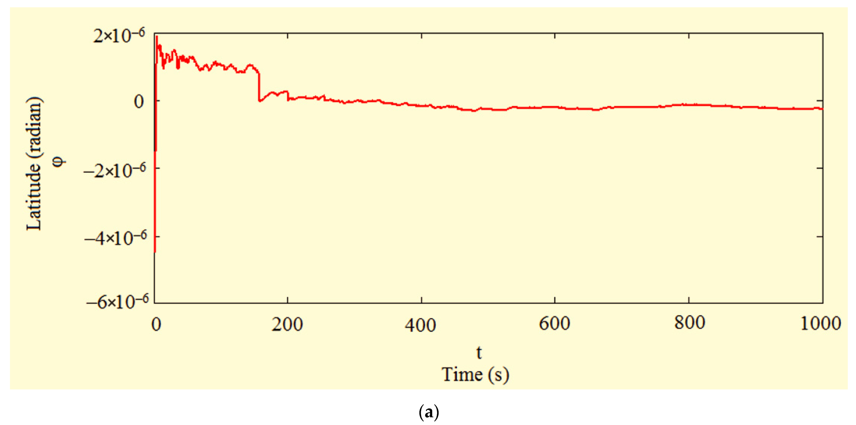
Numerical Solving the Adaptive Assessment of Navigation Parameters of an Unmanned Vehicle

Currently, one of the problems hindering the widespread use of an unmanned vehicle (UV) is the problem of ensuring their high-precision positioning by noisy measurements of the satellite navigation system in conditions of intense urban interference. At the same time, in urban conditions, it is easy to organize active information points with precisely known coordinates (beacons, optical reference points, etc.), which can provide the navigation system of unmanned vehicles with additional accurate positional measurements. In this regard, we will consider in this aspect the possibility of improving the accuracy of solving the navigation problem of an unmanned vehicle based on the proposed approach.
When solving the navigation problem, the UV-Equations of its navigation parameters (latitude and longitude) in the geographical coordinate system (GCS) had the following form:
φ ˙ = V y ( r + h ) , λ ˙ = V x cos ϕ ( r + h ) ,
where φ and λ are geographical UV-latitude and UV-longitude, r is the radius of the Earth, h is the UV-altitude above sea level, and Vy, Vx are the linear UV-velocity projections on the GCS-axes.
The following data were determined as the initial data for modeling:
  • Starting point coordinates of the UV-movement φ0 = 0.76 rad and λ0 = 0.32 rad;
  • Time interval [0; 1000] s;
  • UV-movement constant velocity V = 18 m s−1;
  • UV-trajectory along the Earth’s surface is loxodromic with an azimuthal angle A = 0.23 rad;
  • Random height h changes generated by the trajectory relief are distributed according to the Gaussian law with zero mean and dispersion Gh = (0.14 m)2;
  • Type of UV navigation system is satellite-based.
Based on the initial conditions, the UV-velocity projections on the GSK-axis are determined as follows:
V x = V sin A , V y = V cos A .
According to satellite messages received by the UV navigation system with a τ = 0.1 s clock cycle, navigation measurements are formed along longitude λ and latitude φ channels with a covariance matrix of measurement noise R = | 4 10 10 0 0 9 10 10 | .
Since a given UV-movement velocity causes a slight change in its coordinates at a given time interval, it turns out to be advisable to use instead of the general navigation Equation (10) their linearized version:
φ ˙ ( t ) = V y ( r + 2 h 0 ) ( r + h 0 ) 2 V y ( r + h 0 ) 2 h   , λ ˙ ( t ) = V x cos φ 0 ( r + h 0 ) [ r + 2 h 0 r + h 0 s i n φ 0 φ 0 cos φ 0 ] V x cos φ 0 ( r + h 0 ) 2 h + + V x s i n φ 0 cos 2 φ 0 ( r + h 0 ) φ ,
where h0 = 0.
Equation (11) of true UV-movement was integrated by the Runge–Kutta method of the fourth order with a step of 0.001 s. Each 100th value was used to form satellite measurements (additive overlay of the corresponding noise of satellite navigation measurements) and for subsequent comparison with the estimates obtained.
The discrete Kalman filter, constructed according to the linearized equation (11) of UV-movement, has the following form:
ξ ^ i + 1 = Φ i + 1 / i ξ ^ i + Ω i + 1 + K i + 1 ( z i + 1 H i + 1 Φ i + 1 / i ξ ^ i ) , ξ ^ i = | φ ^ i λ ^ i | , Φ i + 1 i = | 10 τ V x t g φ 0 r cos φ 0 1 | , Ω i + 1 = | τ V y r τ V x r cos φ 0 ( 1 φ 0 t g φ 0 ) | , G i + 1 = | ( V y r 2 ) 2 τ 2 G h V y r 2 V x r 2 cos φ 0 τ 2 G h V y r 2 V x r 2 cos φ 0 τ 2 G h ( V x r 2 cos φ 0 ) 2 τ 2 G h | , H i + 1 = | 1   0 0   1 | .
When moving along the trajectory, the UV crossed points with exactly known coordinates λ and φ (traffic lights—radio beacons) at 150, 158, 250, and 255 s. Up to 158 s, the error δH in determining the measurement matrix was set as an additive matrix δ H = | 0.31   0.04 0.05   0.28 | , from the 200th to the 255th s, respectively, as δ H = | 0.11   0.015 0.03   0.12 | . According to the proposed approach, the exact values of λ and φ at the 158th and 255th s were used to determine the values of the components of the δH matrices, which were then used to correct the measurement matrix in the filter (12).
Modeling of the UV-movement and evaluation of its navigation parameters was carried out for 100 variants of trajectory modeling and evaluation of its parameters for both correctable and noncorrectable measurement matrices.
The graphs of errors in estimating navigation parameters obtained by implementing the filter (12) for a typical case of estimation with an uncorrectable measurement matrix are shown in Figure 1. In this case, the errors in the estimates of the current coordinates of the BA are very significant: at the end of the modeling interval, the error in estimating latitude reached 33.8 m, with a tendency for a further sharp increase (longitude—9 m), also having a divergent character. Moreover, the statistical analysis of estimation errors carried out for all modeling variants showed that the average variance of the deviation relative to the true values of the navigation parameters reaches 650 m2.
When organizing an adaptive filter in accordance with the above algorithm, the estimation errors for the same modeling variant have the form shown in Figure 2.
In this case, it can be seen that the use of the proposed algorithm led to a sharp decrease in estimation errors compared to the traditional Kalman filter—up to 1.2 m in latitude and 1.12 m in longitude. At the same time, such a sharp decrease in errors begins already from about the 500th s while having a pronounced stable character until the end of the modeling interval. Statistical analysis of estimation errors for the proposed algorithm showed that in this case, the average variance of the deviation relative to the true values of the navigation parameters does not exceed 3 m2, which is much more accurate than the traditional filtering scheme.

4. Conclusions

The sharp difference between the statistical estimates of the average variances of deviations relative to the true values of the navigation parameters obtained using the classical Kalman and the proposed filtering algorithms allows us to conclude about the advantages of the latter, despite such a disadvantage as a slight increase in computational costs. In general, the simplicity and accuracy of the proposed algorithm provide the possibility of its effective application for the widest class of information and measurement systems. Moreover, based on this approach, developed by complexing two fundamentally different methods, the use of irregular accurate observations of the object’s state vector and the mathematical apparatus for the study of disturbed multidimensional linear systems, it is possible to further generalize the identification procedure to the remaining parameters of the Kalman filter, in particular the covariance matrices of object noise and measurements, which will further improve the accuracy and stability of the filtration process as a whole.

Author Contributions

Conceptualization, S.V.S. and A.A.M.; methodology, S.V.S., A.A.M., D.N.D. and M.V.P.; formal analysis, S.V.S., M.V.P. and A.I.N.; investigation, S.V.S. and A.A.M.; data curation, T.P.N., D.N.D. and M.V.P.; writing—original draft preparation S.V.S., A.A.M., M.V.P., T.P.N., D.N.D. and A.I.N.; writing—review and editing S.V.S., A.A.M., M.V.P., T.P.N. and A.I.N.; validation A.A.M., S.V.S., D.N.D. and T.P.N.; visualization, T.P.N. and D.N.D.; supervision, S.V.S. All authors have read and agreed to the published version of the manuscript.

Funding

This research received no external funding.

Data Availability Statement

Data sharing not applicable.

Conflicts of Interest

The authors declare no conflict of interest.

References

  1. Fan, Y.; Xu, K.; Wu, H.; Zheng, Y.; Tao, B. Spatiotemporal Modeling for Nonlinear Distributed Thermal Processes Based on KL Decomposition, MLP and LSTM Network. IEEE Access 2020, 8, 25111–25121. [Google Scholar] [CrossRef]
  2. Urrea, C.; Agramonte, R. Kalman Filter: Historical Overview and Review of Its Use in Robotics 60 Years after Its Creation. J. Sens. 2021, 2021, 9674015. [Google Scholar] [CrossRef]
  3. Sinitsyn, I.N. Kalman and Pugachev Filters; Logos: Moscow, Russia, 2007; ISBN 978-5-98704-270-4. (In Russian) [Google Scholar]
  4. Rovira, E.; McGarry, K.; Parasuraman, R. Effects of imperfect automation on decision making in a simulated command and control task. Hum. Factors: J. Hum. Factors Ergon. Soc. 2007, 49, 76–87. [Google Scholar] [CrossRef] [PubMed]
  5. Buscarino, A.; Fortuna, L.; Frasca, M.; Muscato, G. CHAOS DOES HELP MOTION CONTROL. Int. J. Bifurc. Chaos 2007, 17, 3577–3581. [Google Scholar] [CrossRef]
  6. Liu, T.-H.; Wen, Y.-L.; Li, G.-Q.; Nie, X.-N. Optimization and Experimental Study of an Intelligent Bamboo-Splitting Machine Charging Manipulator. J. Robot. 2020, 2020, 4675301. [Google Scholar] [CrossRef]
  7. Bucolo, M.; Buscarino, A.; Fortuna, L.; Famoso, C. Stochastic resonance in imperfect electromechanical systems. In Proceedings of the 2020 IEEE 29th International Symposium on Industrial Electronics (ISIE), Delft, The Netherlands, 17–19 June 2020; pp. 210–214. [Google Scholar] [CrossRef]
  8. Bucolo, M.; Buscarino, A.; Famoso, C.; Fortuna, L.; Frasca, M. Control of imperfect dynamical systems. Nonlinear Dyn. 2019, 98, 2989–2999. [Google Scholar] [CrossRef]
  9. Chen, W.-H.; Yang, J.; Guo, L.; Li, S. Disturbance-Observer-Based Control and Related Methods—An Overview. IEEE Trans. Ind. Electron. 2015, 63, 1083–1095. [Google Scholar] [CrossRef] [Green Version]
  10. Hartley, R.; Ghaffari, M.; Eustice, R.M.; Grizzle, J.W. Contact-aided invariant extended Kalman filtering for robot state estimation. Int. J. Robot. Res. 2020, 39, 402–430. [Google Scholar] [CrossRef]
  11. Zhong, Y.; Zhang, W.; Zhang, Y.; Zuo, J.; Zhan, H. Sensor Fault Detection and Diagnosis for an Unmanned Quadrotor Helicopter. J. Intell. Robot. Syst. 2019, 96, 555–572. [Google Scholar] [CrossRef]
  12. Hsieh, C.-S.; Chen, F.-C. Optimal Solution of the Two-Stage Kalman Estimator. IEEE Trans. Automat. Contr. 1999, 44, 194–199. [Google Scholar] [CrossRef] [Green Version]
  13. Oveisi, A.; Nestorovic, T. Mixed Kalman-Fuzzy Sliding Mode State Observer in Disturbance Rejection Control of a Vibrating Smart Structure. Int. J. Acoust. Vib. 2019, 24, 677–686. [Google Scholar] [CrossRef]
  14. Rana, R.; Agarwal, V.; Gaur, P.; Parthasarathy, H. Design of Optimal UKF State Observer–Controller for Stochastic Dynamical Systems. IEEE Trans. Ind. Appl. 2020, 57, 1840–1859. [Google Scholar] [CrossRef]
  15. Tan, J.; Xu, F.; Wang, X.; Yang, J.; Liang, B. Invariant set-based robust fault detection and optimal fault estimation for discrete-time LPV systems with bounded uncertainties. Int. J. Syst. Sci. 2019, 50, 2962–2978. [Google Scholar] [CrossRef]
  16. Li, J.; Wang, Z.; Zhang, W.; Raissi, T.; Shen, Y. Interval observer design for continuous-time linear parameter-varying systems. Syst. Control. Lett. 2019, 134, 104541. [Google Scholar] [CrossRef]
  17. Wan, Y.; Keviczky, T. Real-time nonlinear moving horizon observer with pre-estimation for aircraft sensor fault detection and estimation. Int. J. Robust Nonlinear Control 2017, 29, 5394–5411. [Google Scholar] [CrossRef]
  18. Minowa, A.; Toda, M. A High-Gain Observer-Based Approach to Robust Motion Control of Towed Underwater Vehicles. IEEE J. Ocean. Eng. 2018, 44, 997–1010. [Google Scholar] [CrossRef]
  19. Novi, T.; Capitani, R.; Annicchiarico, C. An integrated artificial neural network—Unscented Kalman filter vehicle sideslip angle estimation based on inertial measurement unit measurements. Proc. Inst. Mech. Eng. Part D J. Automob. Eng. 2018, 233, 1864–1878. [Google Scholar] [CrossRef]
  20. Sasiadek, J.Z.; Wang, Q. Low cost automation using INS/GPS data fusion for accurate positioning. Robotica 2003, 21, 255–260. [Google Scholar] [CrossRef] [Green Version]
  21. Hide, C.; Moore, T.; Smith, M. Adaptive Kalman filtering algorithms for integrating GPS and low cost INS. In Proceedings of the PLANS 2004. Position Location and Navigation Symposium, Monterey, CA, USA, 26–29 April 2004; pp. 227–233. [Google Scholar] [CrossRef]
  22. Herrera, E.P.; Kaufmann, H. Adaptive methods of Kalman filtering for personal positioning systems. In Proceedings of the 23rd International Technical Meeting of the Satellite Division of the Institute of Navigation, Portland, OR, USA, 21–24 September 2010. [Google Scholar]
  23. Mohamed, A.H.; Schwarz, K.P. Adaptive Kalman Filtering for INS/GPS. J. Geod. 1999, 73, 193–203. [Google Scholar] [CrossRef]
  24. Looney, M. Optimization of navigation characteristics of the mobile robot. Compon. Technol. 2012, 126, 48–50. [Google Scholar]
  25. Litvin, M.A.; Malyugina, A.A.; Miller, A.B.; Stepanov, A.N.; Chickrin, D.E. Error Classification and Approximation in Inertial Navigational Systems. Inf. Process. 2014, 14, 326–339. [Google Scholar]
  26. Hu, C.; Chen, W.; Chen, Y.; Liu, D. Adaptive Kalman Filtering for Vehicle Navigation. J. Glob. Position. Syst. 2003, 2, 42–47. [Google Scholar] [CrossRef] [Green Version]
  27. Reznichenko, V.I.; Maleev, P.I.; Smirnov, M.Y. The satellite correction of orientation parameters for marine objects. Navig. Hydrogr. 2008, 27, 25–32. [Google Scholar]
  28. Tsyplakov, A.A. An Introduction to State Space Modelling. Quantile 2011, 2011, 1–24. [Google Scholar]
  29. Mehra, R. On the identification of variances and adaptive Kalman filtering. IEEE Trans. Autom. Control. 1970, 15, 175–184. [Google Scholar] [CrossRef]
  30. Velikanova, E.P.; Voroshilin, E.P. Adaptive estimating of maneuvering object position in changeable radio channel transmission gain. Dokl. Tomsk. Gos. Univ. Sist. Upr. I Radioèlektroniki 2012, 26, 29–35. (In Russian) [Google Scholar]
  31. Shilina, V.A. Inertial Sensor System for Indoor Navigation. Available online: http://ainsnt.ru/doc/778220.html (accessed on 5 January 2020).
  32. Sokolov, S.; Polyakova, M.V.; Kucherenko, P.A. Analytic Synthesis of a Kalman Adaptive Filter on the Basis of Irregular Precise Measurements. Meas. Tech. 2018, 61, 232–237. [Google Scholar] [CrossRef]
  33. Sokolov, S.V.; Novikov, A.I. Adaptive estimation of UVs navigation parameters by irregular inertial-satellite measurements. Int. J. Intell. Unmanned Syst. 2020, 9, 274–282. [Google Scholar] [CrossRef]
  34. Sokolov, S.; Novikov, A.; Polyakova, M. Adaptive Stochastic Filtration Based on the Estimation of the Covariance Matrix of Measurement Noises Using Irregular Accurate Observations. Inventions 2021, 6, 10. [Google Scholar] [CrossRef]
  35. Chernov, A.A.; Yastrebov, V.D. Disturbances of the Kalman filtering process. Cosm. Res. 1984, 22, 12–19. [Google Scholar]
Figure 1. Graphs of latitude φ (a) and longitude λ (b) estimation errors obtained when implementing the classical Kalman filter.
Inventions 06 00080 g001aInventions 06 00080 g001b
Figure 2. Graphs of latitude φ (a) and longitude λ (b) estimation errors obtained when implementing the adaptive filter.
Inventions 06 00080 g002aInventions 06 00080 g002b
Publisher’s Note: MDPI stays neutral with regard to jurisdictional claims in published maps and institutional affiliations.

