
A Novel 2-D Point Absorber Numerical Modelling Method


1
Department of Civil Engineering, Faculty of Engineering of the University of Porto (FEUP), 4200-465 Porto, Portugal
2
Interdisciplinary Centre of Marine and Environmental Research of the University of Porto (CIIMAR), 4200-465 Porto, Portugal
3
Department of Naval Architecture, Ocean and Marine Engineering, University of Strathclyde, Glasgow G4 0LZ, UK
*
Author to whom correspondence should be addressed.
Inventions 2021, 6(4), 75; https://doi.org/10.3390/inventions6040075
Submission received: 29 September 2021
/
Revised: 25 October 2021
/
Accepted: 27 October 2021
/
Published: 29 October 2021
(This article belongs to the Special Issue Marine Renewable Energy, an Important Resource Towards a Low Carbon Future)
Abstract
:Despite several wave energy converters (WECs) having been developed to present, no particular concept has emerged yet. The existing inventions vary significantly in terms of the operation principle and complexity of WECs. The tethered point absorbers (PAs) are among the most known devices that, thanks to their simplicity, appear to be cost-effective and reliable for offshore installation. These devices need to be advanced further and, therefore, new tailored modelling methods are required. Numerical modelling of this type of WEC has been done mainly in one degree of freedom. Existing methods for multi-degrees of freedom analysis lack pragmatism and accuracy. Nevertheless, modelling of multiple degrees of freedom is necessary for correct analysis of the device dynamic response, wave loads and device performance. Therefore, an innovative numerical method for two degrees of freedom analysis of PA WECs, which permits precisely modelling the dynamics of PA for surge and heave motions, is introduced in this paper. The new method allows assessing, in the time-domain, the dynamic response of tethered PAs using regular and irregular sea states. The novel numerical model is explained, proved and empirically validated.
1. Introduction
Along most ocean coasts, a vast wave power resource that can be harnessed for electricity production exists. This resource is estimated to be about 2.11 TW [1], which is significantly more than the one of tidal energy that is limited to a few locations [2,3]. Throughout the present and previous centuries, many have tried to invent efficient and reliable wave energy converters (WECs) that could be cost-effective for large-scale energy production. WEC inventions have been so numerous that the wave energy sector can be informally called the ‘’inventors’ paradise’’ [4]. However, to present, the WECs that reached a high technology readiness level and good commercial progress are very few. Within the most promising WEC concepts, there are oscillating water columns [5,6], oscillating body or pivoting WECs [7,8,9,10,11], overtopping devices [12,13,14] and offshore point absorbers (PAs) [15,16,17]. The latest, due to reliability and minimal complexity, represent an important class of WECs [18].
Offshore WECs need to be located at offshore locations where high wave energy occurs. Therefore, these WECs are exposed to highly repetitive and significant structural loads. These loads are primarily due to the waves acting on the floating part of the WEC, which are transmitted to the mooring cable(s). If this last component fails, the WEC would drift away and may cause significant safety problems and economic losses. Examples of offshore WECs are illustrated in Figure 1. These WECs can be categorized into two main clusters, earth-reacting and self-reacting, and into two more subgroups, floating at the surface [19,20,21,22,23,24] or fully submerged [25,26]. The mooring component must counteract loads that are equivalent in magnitude and characteristics to the environmental forces acting on the WEC. The problem of quantifying such mooring loads is an old one that has always existed in the traditional offshore industry for the design of stationing vessels and offshore structures moored for oil and gas production. However, there are significant differences between the problem of mooring WECs and the problem of mooring vessels and traditional offshore platforms [27]. On one hand, some of the existing knowledge can be applied, to some extent, to the new problem related to WECs’ mooring design [28]. On the other hand, new approaches are required due to the special characteristics of WECs. In general, mooring systems for ships and conventional structures have been designed, in the past, using simplified static or quasi-static design approaches that considered the floating structure to be almost motionless. Due to the nature of WECs, the application of these approaches does not necessarily lead to good design results. In addition, dynamics-based methods for the traditional type of structures are generally complex and applicable only to specific cases. Even if these methods may be applicable, they are often over-complicated to implement. Therefore, there is a need for practical new methods based on dynamic approaches that should be suitable for the particular requirements of WECs.
Given the aforementioned context, in this paper, an innovative numerical method for the analysis of earth-reacting WECs is proposed, described, verified and validated with experimental data for a PA theoretical device. The numerical method allows assessing the dynamic response of a PA under different types of wave loads. This novel modelling method can be useful for the development of the design of PAs and similar devices, for instance, by targeting the best design parameters for maximizing the energy absorption performance by means of studying the WEC response for recurrent ocean conditions. Initially, all relevant materials and methods will be covered (Section 2), successively results are discussed (Section 3) and conclusions are provided (Section 4).
2. Materials and Methods
In this section, at first, PA devices are introduced, and relevant studies are briefly described (Section 2.1). Next, the characteristics of the theoretical device considered are described and the relevant theory is presented (Section 2.2 and Section 2.3). Subsequently, the innovative approach for 2-D PA numerical modelling is explained (Section 2.4, Section 2.5, Section 2.6 and Section 2.7). Finally, new experiments carried out for gathering the valuable data needed for numerical results validation and the uncertainty analysis of experimental data are described and the main details presented (Section 2.8 and Section 2.9).
2.1. Point Absorber Wave Energy Converters
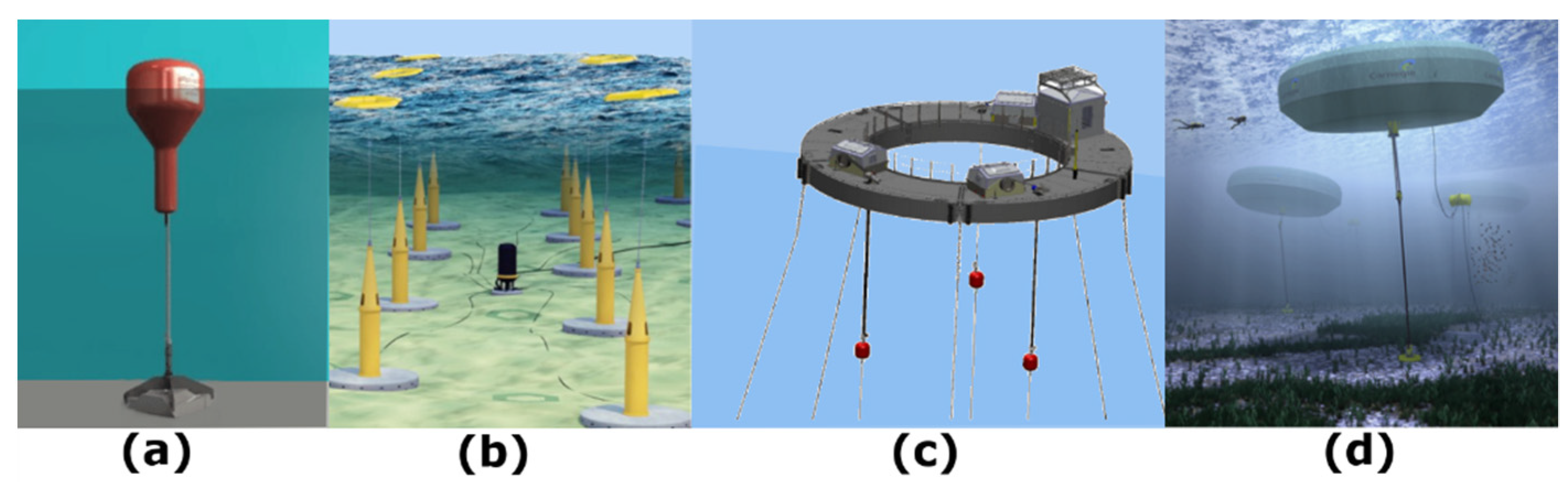
PAs, compared to other types of WECs, present various advantages. In general, their small dimensions may allow lower capital costs and experience reduced extreme wave loads due to a limited WEC external total surface. Examples of offshore PAs are illustrated in Figure 2. These devices are made of a single floater that is connected to the seabed by means of straight tethers. The floater, thanks to wave loads, activates a power take-off (PTO) system, which can be a direct drive (electromagnetic) or hydraulic type of generator. Specifically for PAs, various recent studies point out the importance of the generator unit selection [29] focusing on the best materials to use [30,31] and on electromagnetic PTO winding design [32]. Another key topic of research is the development of PTO control techniques to apply for significantly increasing the power absorption efficiency, e.g., reactive or latching control strategies [33,34,35].
For what concerns numerical and experimental modelling of PAs, a limited number of studies have been published so far. Since using only frequency-domain analysis approaches can lead, in general, to very approximated results, a time-domain method is recommended [36,37,38,39]. Significant mathematical and numerical difficulties exist for the development of a two or more degrees of freedom model of a WEC system, including a restoring spring and damping components representing the PTO system [40]. Past methods concern rather difficult implementation and, in most cases, were not validated with experimental results. Nevertheless, to assess the validity of a numerical model for WEC simulation, it is imperative to compare results with empirical evidence.
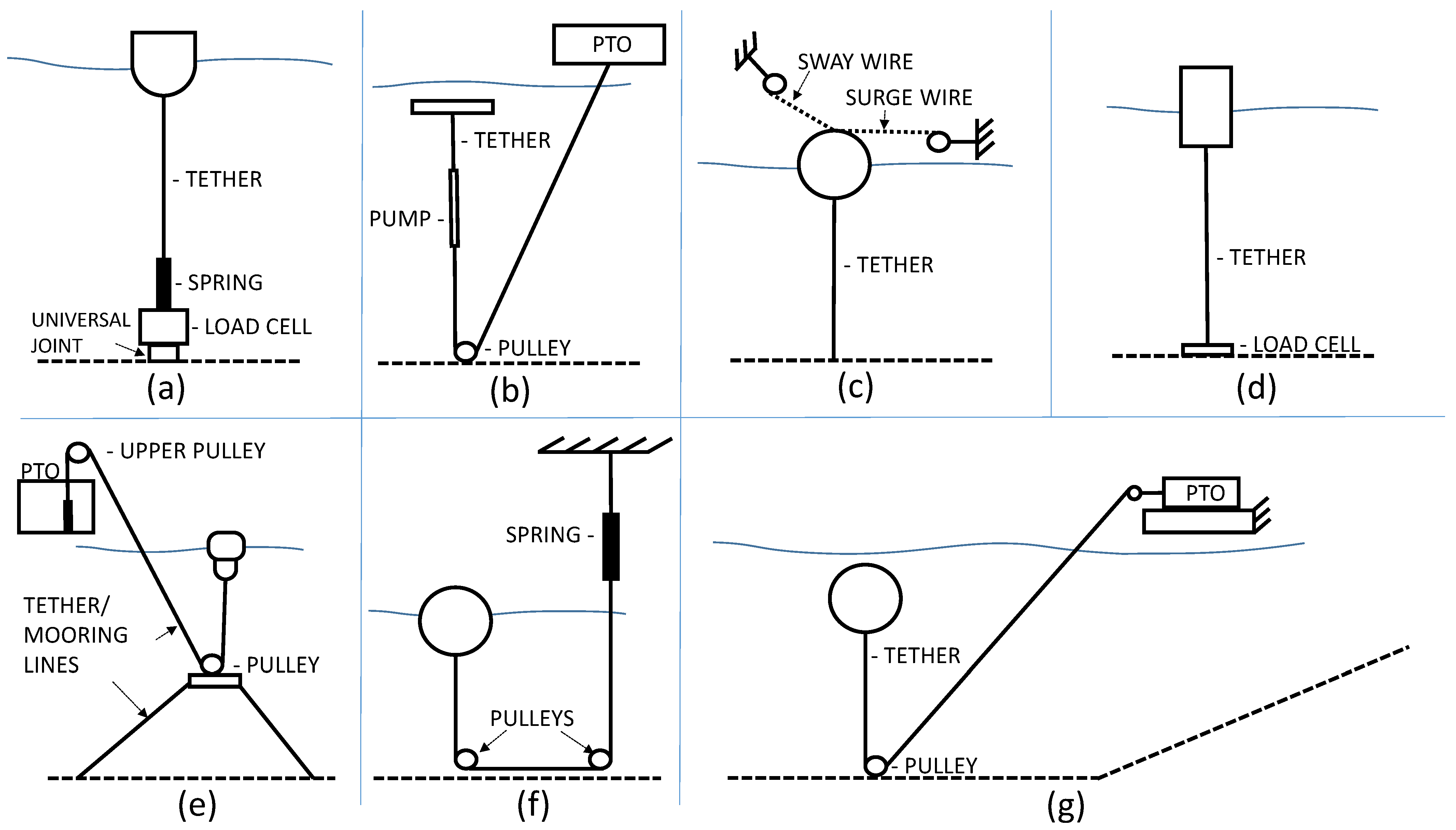
Taut moored devices such as PA were studied empirically by a few researchers. Particular difficulties exist in physically modelling the PTO system at model scale [41]. In Figure 3, the schemes of experimental setups that were assembled during previous works are reported. With a particular focus on extreme loads and responses, in [42,43], PA WECs were studied through experiments on model scale devices (Figure 3a,b). The findings of the first study, related to snatch loading, indicated that the magnitude of extreme loading is not very dependent on the wave steepness, but body motion and displacement influence is significant. The second study concerned the specific Ceto WEC and also investigated mostly extreme loading. While [42] investigating extreme loading by increasing wave steepness and using breaking and non-breaking waves, defined with the NewWave theory, [43] used long irregular sea simulations and a numerical model for investigating mainly maximum PTO extensions. Other authors studied the instability of tethered floaters without PTO components. These studies concerned the analysis of the nonlinear body motion with free oscillations and waves tests. Experimental and theoretical work for finding Mathieu’s instability diagram was carried out [44], being the scaled models of this study reported in Figure 3c,d. In contrast, in [45], the authors used a moored floating sphere with a spring component for understanding the validity of the Smoothed Particle Hydrodynamics (SPH) theory for modelling surface and structure interaction, Figure 3f. In this study, valuable guidelines for correctly using SPH theory for studying such types of fluid-structure interaction problems are provided. For numerical models, in [46] and [47], experimental work on scaled models of the Ceto and CorPower WECs are described, respectively. The experimental setups are shown in Figure 3e,g. Both studies accurately compared numerical and experimental results. While in the first study CFD methods, requiring high computational resources, are applied for modelling the device, the second concerns a numerical model based on the Cummins equation [48], which instead requires low computational resource requirements. For both studies, extended experimental work was carried out with laboratory models consisting of a floater and PTO assemblies. The PTO system for the Ceto model was minimized to a controlled servomotor, which was emulating the desired combined spring-damping effect. For the CorPower WEC model, the PTO damping and spring effects, more practically, were simulated mechanically. In this case, the negative spring force was exerted with originality by an element made by specific cylindrical pneumatic components.
2.2. Point Absorber Model Characteristics
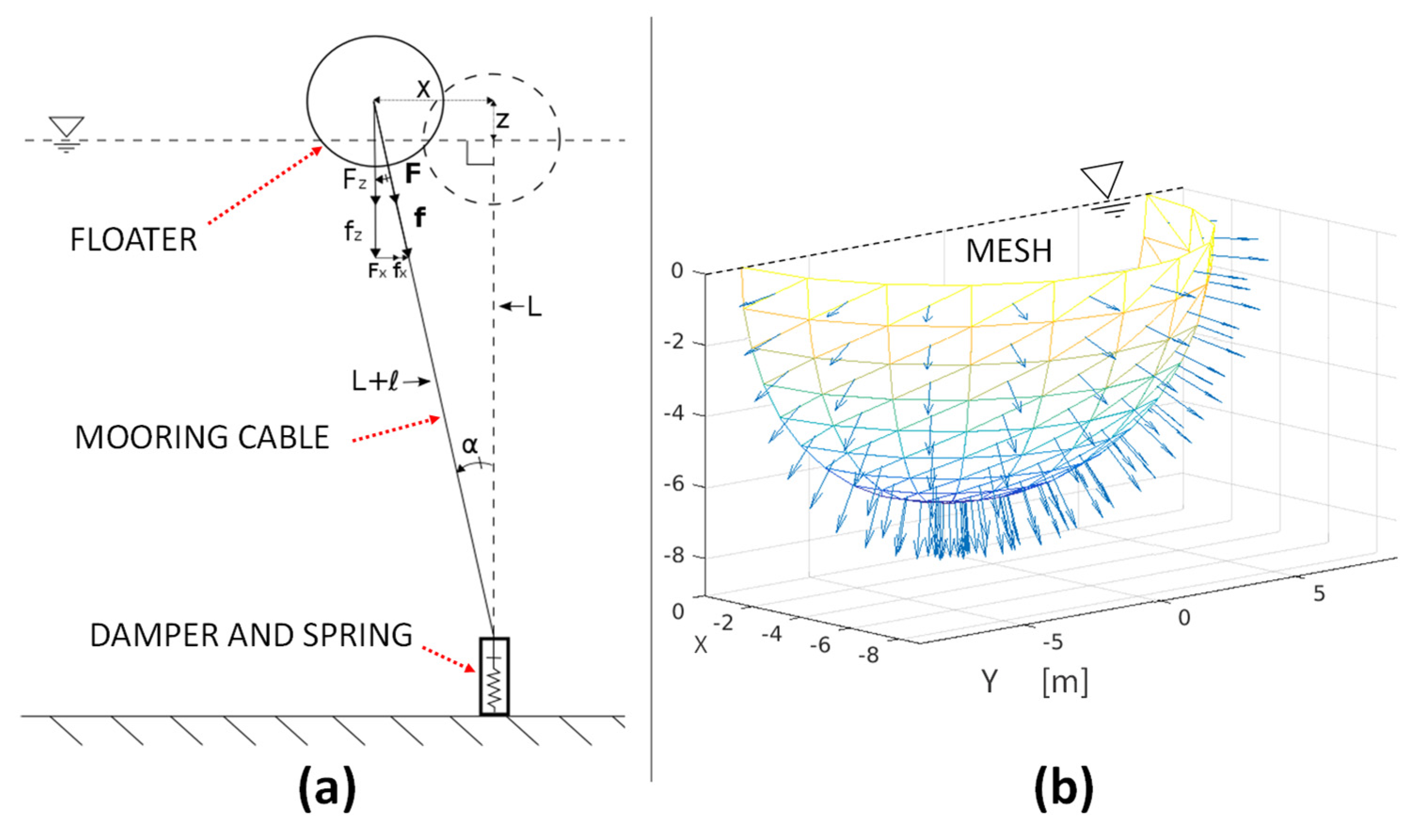
The point absorber (PA) model illustrated in Figure 4a is defined for demonstrating the innovative numerical modelling method. This PA is a theoretical device formed by a spherical floater, a mooring line and a PTO represented by spring and damper components. The axial displacement of the mooring line occurring due to compression or extension of the spring component is denoted by ℓ. The force exerted by the spring and damper components, excluding the pretension load, is denoted by f. Considering this geometry, the mooring restoring force can be defined as, where and are the horizontal and vertical components of the force, which are:
where , and are the pretension load and the corresponding horizontal and vertical components, respectively. Instead, f can be found using,
Note that ℓ is found by applying the Pythagorean Theorem, giving
. Thus, ℓ is found to be:
is found to be:
Further note that: and .
The floater is set to have a draft equal to its radius , and its mass is defined as, where is the water density and the gravitational acceleration.
2.3. Linear Frequency-Domain Analysis
For defining the frequency-domain equations, the mooring components are linearized. To do so, it is assumed that only small surge displacements occur at all times, and α is a small angle. Thus, it can be assumed that and the horizontal mooring force component can be approximated as: . For what concerns the heave component, this is defined as , where is the vertical restoring force due to spring stiffness, and is the PTO force.
Taking into account surge and heave () motions and including the linearized effects of the damper-spring system, the following equations are defined [37]:
where is the mass, and are the added mass coefficients, and are the radiation damping coefficients, the mooring pretension, is the length of the mooring line, is the PTO damping constant, is the spring stiffness constant, is the water density, is gravitational acceleration, is the cross-sectional area of the spherical floater () and and are the components of the wave excitation force.
By substituting , and ordering terms, Equation (6) is converted in Equation (7), where mooring stiffness and PTO damping are included in stiffness K and damping C matrices. This last equation gives the solution in terms of displacements when the frequency-domain approach is implemented.
2.4. Time-Domain Formulation
The time-domain formulation is possible by implementing the theory developed by Cummins [48], who derived the general equation of motions for a floating body by introducing convolution integrals. The methodology implemented is normally used for sea-keeping applications. In particular, the added mass and radiation damping coefficients can be calculated independently. This operation is possible thanks to further findings of Ogilvie [49], who derived the equations of motion for a ship separating the radiation and diffraction problems. In practice, the hydrodynamic coefficients can be calculated with a Boundary Element Code, for instance, NEMOH [50,51]. The time-domain formulation adopted may be referred to as the ‘weakly nonlinear time-domain method’. For the two-dimensional case, the equations for surge and heave motions can be written as follows:
where is the mass, the added mass values for , and and the horizontal and vertical components of the mooring restoring force, respectively. and represent the floater’s surge and heave displacements. Two over-dots indicate accelerations (second-order derivative). The is the casual kernel function present in convolution integrals, which represents the memory effect of the radiation forces. This function is evaluated for a short period that embodies system response in a previous interval (actual time step minus a defined short period of c.a. 20 s for the WEC analyzed). The following formula defines the kernel function:
The mooring force components for the two-dimensional PA case can be defined as previously introduced in Equations (1) and (2), i.e., and
. These mooring force components depend on: floater’s displacements and velocities, the spring stiffness coefficient, , the PTO damping, , the mooring length, , and the mooring pretension, . The advantage of the adopted theory compared to the frequency-domain approach is that transient effects, for example, existing due to the presence of the PTO mechanism or the mooring system, can be captured in the methodology. For the formulation to be valid, it is assumed that displacements are small and that these are directionally proportional to the induced velocity of the water particles surrounding the body and vice versa. In practice, having assumed that only small displacements occur and that the fluid is potential, the superimposition principle can be applied.
2.5. First-Order Wave Loads
Wave excitation forces coefficients can be calculated with a code based on the Boundary Element Method (BEM) and used to compute the time-dependent first-order wave loads in both regular and irregular sea states. For defining the wave excitation forces, two methods can be used. The first, named ‘direct wave loading option’ (DWLO), is based on the superimposition principle. While, for regular waves, the sea is assumed sinusoidal, for the irregular sea case a force vector is created by adding together different sinusoidal functions of various amplitudes and frequencies. In contrast, a second option, named ‘impulse-response wave loading option’ (IRWLO), concerns the application of the impulse-response functions. These last functions—similar to the computation of the radiation forces—are used with the IRWLO for calculating the waves excitation load terms. For this second option, the wave loads in regular and irregular seas depend excursively on the free surface signal . The latter can be determined either with the DWLO or by using a defined free surface elevation vector, which can be obtained from real sea measurements or by hydrodynamic tank tests measurements.
For DWLO, the regular waves force can be assumed to be varying in a sinusoidal way. For the irregular sea option, a sea spectrum, such as the Bretschneider, should be adopted. This spectrum is defined as [52]:
The above, when used for the particular case of , reduces to the one-parameter Pierson-Moskowitz wave spectrum. This spectrum is simpler to implement compared to other types of spectra and is representative of the Atlantic Ocean conditions. This spectrum does not require any other particular parameter except the representative wave period and significant wave height .
Differently for IRWLO, the wave loads, for both regular and irregular waves cases, are calculated through the use of the non-casual impulse-response function and the convolution integral, which can be defined as [53]:
where the impulse-response function is equal to:
where is the free surface elevation signal, which represents time in the past and future, and represents wave excitation force coefficients, which are calculated with a BEM code.
2.6. Second-Order Wave Drift Loads
Estimation of drift forces in the time-domain for irregular sea states is done through a technique that concerns the definition of a reflection coefficient, . This factor can be used for calibrating the numerical code and is assessed from regular wave experiments. In practice, for a series of regular wave tests, the surge offset is measured and is defined as the value needed to tune the numerical results. The procedure should be repeated for a sufficient range of regular waves frequencies. The technique developed is comparable to the method proposed by [54], which was also implemented by [55]. The process is based on the assumption that the free surface signal can be seen as a series of single waves. These have amplitudes equal either to the wave crest or to the absolute value of the wave trough. Their wave periods are found by doubling the time between two consecutive zero crossings. When peaks or troughs in between a zero crossing were more than one, an average value is used. The drift force in the time-domain can be then estimated, for both regular and irregular seas, by the following empirical formula:
needs to be evaluated through a computational loop where the two terms and depend on the instantaneous wave period and wave amplitude. The reflection coefficients are interpolated from a vector, which is defined prior to the irregular sea state numerical simulation run.
2.7. Numerical Formulation
The motion of the PA is solved for the two degrees of freedom, namely, heave and surge motions (surge assumed positive towards the waves’ propagation direction). The mooring line is assumed to be connected at the center of the sphere, where also the center of mass is located. It is also supposed that, for the spherical floater, the hydrodynamic coupling between surge and heave directions is negligible.
As mentioned previously, hydrodynamic coefficients, needed for solving the mentioned equation of motion, are obtained with a BEM code (at the beginning of the computation). These include added mass coefficients (), radiation damping coefficients () and wave excitation force coefficients ().
First-order wave excitation loads, for the case of the regular wave, when the DWLO is implemented, can be estimated with the following formula:
The free surface elevation is defined as .
For the case of the irregular wave sea states using the DWLO method, the free surface elevation and the horizontal and vertical components of the wave loads can be instead determined by:
where are wave amplitudes determined by and are random phase values created by defining uniform distributed random numbers between the interval .
As introduced in the previous section, for IRWLO—as for the radiation forces—the wave loads need to be calculated by convolution integrals. Considering Equation (11), defining the casual impulse-response function, and noting that this should be real so that is equal to the complex conjugate , the following equation can be used for the numerical implementation:
where the infinite limits of the above integral for computational efficiency are substituted by limited time values (both negative and positive values). For the considered spherical floater (r = 7.5 m), the decaying time of the above kernel function was to be c.a. ±60 s.
Both casual and non-casual impulse response functions used to solve the convolution integrals, relative to, respectively, the wave excitation loads and the radiation damping forces, are computed similarly. The kernel of convolution integrals related to the radiation forces of the spherical floater considered was vanishing in c.a. 20 s; thus, this value was adopted in the case of the floater considered.
Wave drift forces can only be included in the simulation when excitation IRFs are used. For what concerns the wave drift forces in regular waves simulations, these can be directly estimated with the formula previously introduced (Equation (13)), which is evaluated for each time step of all the simulation time. Diversely, for the irregular sea case, few other operations are carried out before evaluating the mentioned formula. These operations are:
- 1.
- Definition of the free surface elevation signal using an empirical spectrum or by importing a defined from the real-time record;
- 2.
- Finding the points where peaks, through and zero-crossings occur;
- 3.
- Defining a signal of the instantaneous wave period;
- 4.
- Interpolation of vectors found in the previous two steps;
- 5.
- Interpolation of the reflection coefficient, which depends on the instantaneous wave period;
- 6.
- Evaluation of Equation (13);
- 7.
- Adding the found waves drift load vector to the first-order wave load horizontal component vector.
For the time-domain formulation, the vertical direction of the mooring load can be estimated with the following approximation:
This expression is similar to the case of the frequency-domain formulation; only the is added. The is an exponent factor determining the type of damping. To model a linear PTO, this was always set equal to one. Eventually, for simulating a quadratic PTO force, can be set equal to 2. To clarify, the , in this case, is again the PTO damping coefficient. As the mooring line is assumed to be inelastic, this is the only damping taken into consideration in the mooring components terms. and are the heave displacement and heave velocity of the floater. is the spring stiffness constant.
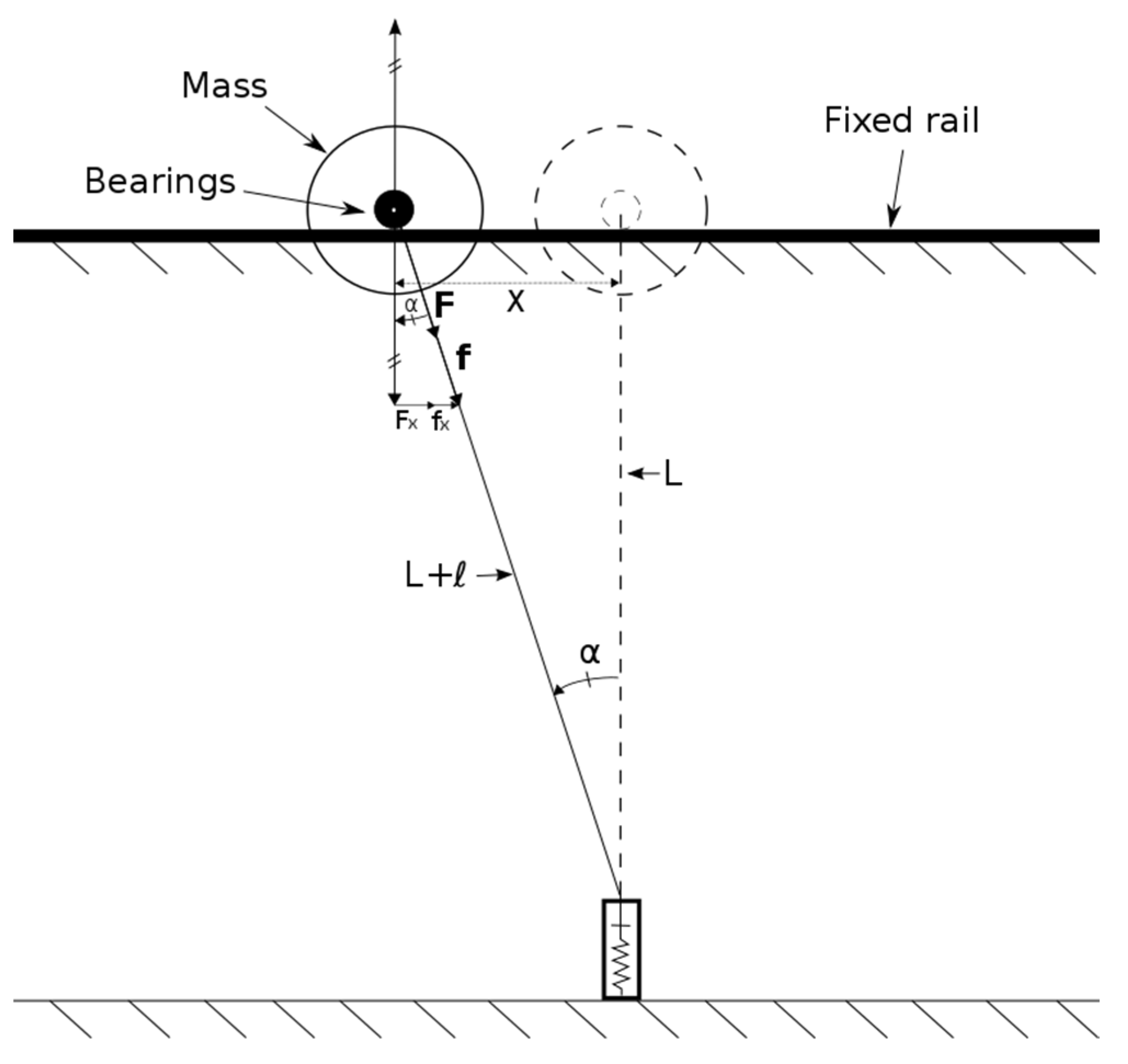
For numerical modelling, the restoring horizontal mooring component the analogue mechanical system, shown in Figure 5, can be considered. This system represents a mass that is attached to a rail through ideal bearings. The mass is free to oscillate along the horizontal direction. The horizontal restoring force is only due to horizontal offset.
Recalling Equations (1) and (3)–(5), the surge component is estimated by assuming that the horizontal restoring force is independent of the floater’s heave velocity and heave position. For surge motion, the mentioned equations become:
Thus, is approximated to be:
where is the spring stiffness, is floater’s surge displacement, is the mooring length, is the PTO damping coefficient, is the mooring pretension and is equal to .
This time, the effect of the PTO damping over the surge motion is considered, not neglected as in the case of the frequency-domain approach.
For the initial period of simulation time, usually a ramping period is required, for instance, this can be set to be 4 times the chosen wave period.
2.8. Experimental Study
For validating the developed numerical model, experiments were carried out with a 1:33 scale physical model at the Kelvin Hydrodynamics Laboratory of the University of Strathclyde, Scotland. Full specifications of this facility are reported in [56]. The main characteristics of the experimental facility are:
- Length = 76 m;
- Width = 4.6 m;
- Depth = 0.5–2.3 m;
- Waves making: variable-water-depth computer-controlled flaps wavemaker;
- Beach: variable-water-depth sloping beach (reflection coefficient typically less than 5%).
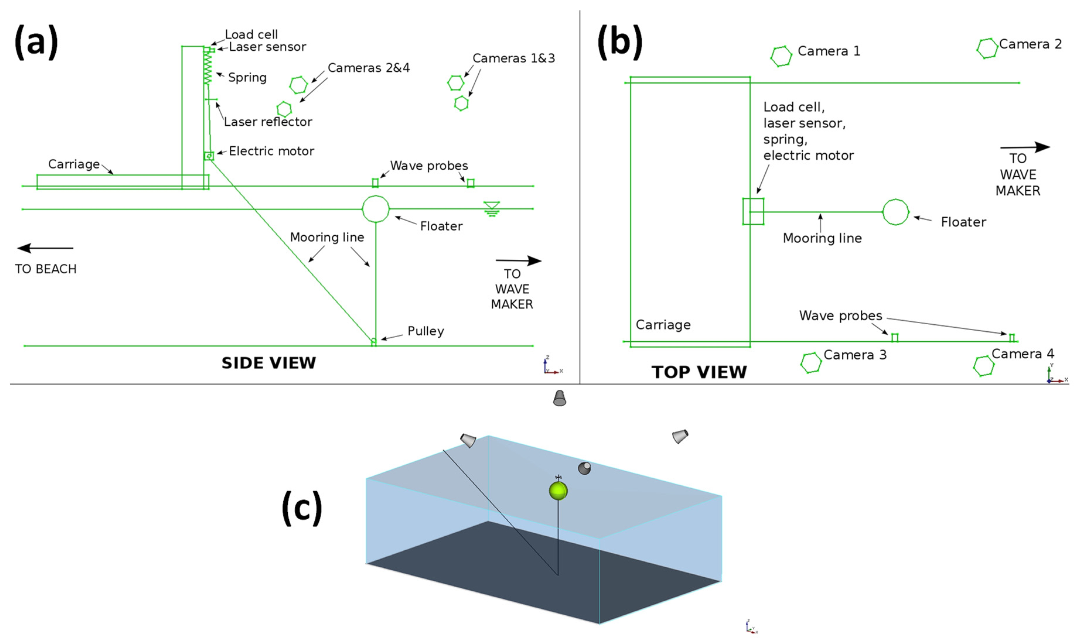
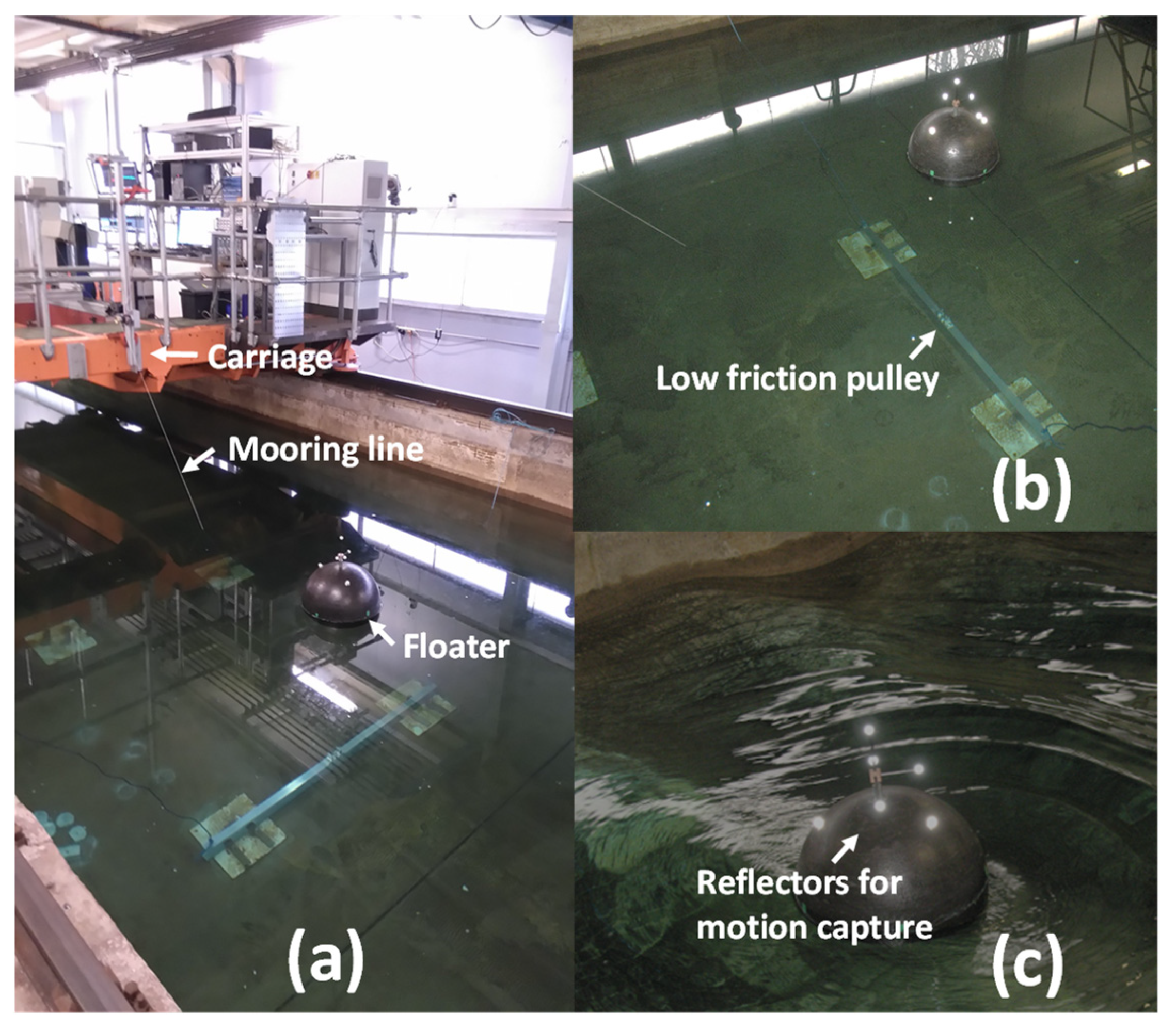
The instruments used and measurements carried out are described in Table 1. For logging floater’s motion in six degrees of freedom, the Qualysis AB motion tracking system was used. Four Qualysis infrared-sensitive cameras were positioned around the tank and directed towards the floater. As can be seen in Figure 6c, the cameras were placed with a certain distance between them to ensure the best capture accuracy. Taking into account the requirements of the Qualysis system, six reflective markers were attached to the floater, Figure 7c. The floater was positioned c.a. 3 m upstream from the carriage, Figure 7a.
The device tested consisted of a spherical floater moored by a single tether, which passed through a pulley at the bottom of the tank (Figure 6a) and attached to the PTO simulation unit. The assembled model parameters are reported in Table 2 (first column), where the mooring length is defined as the distance from the upper part of the pulley to the lower end of the floater ().
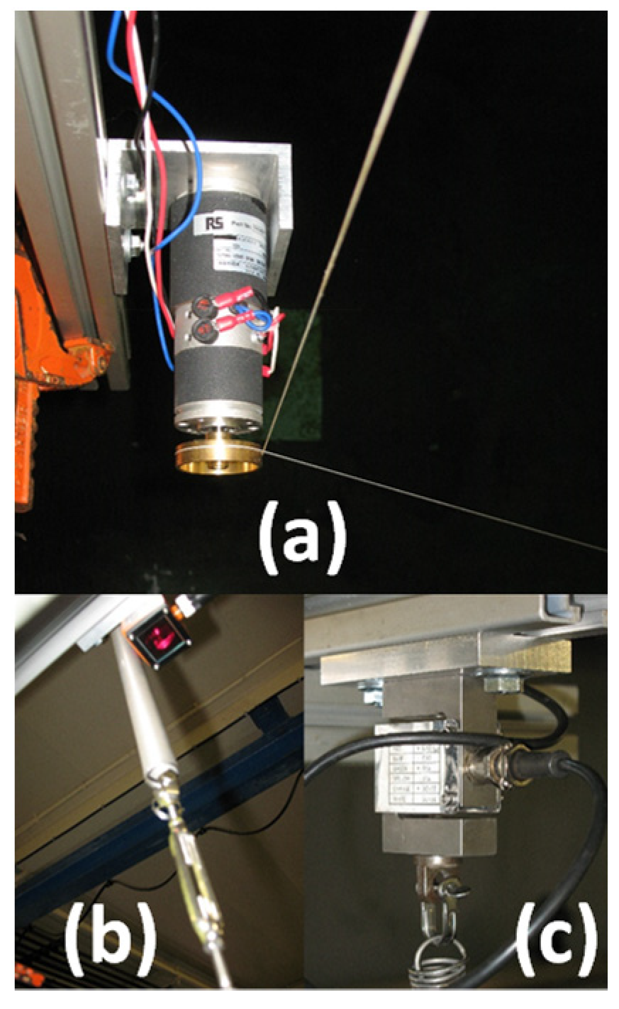
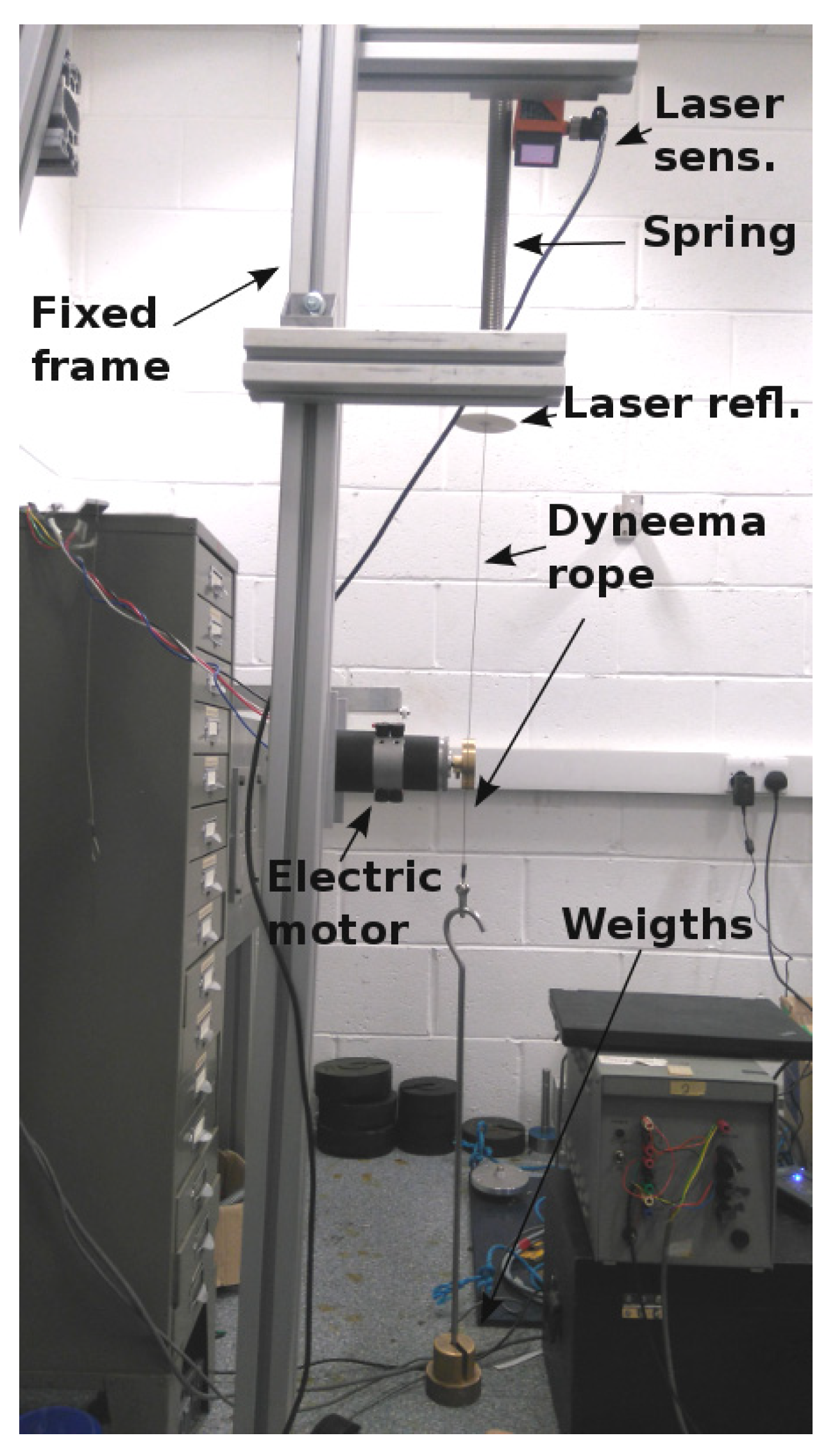
The elongation of the spring (mooring line axial displacement) was measured and recorded by using a laser sensor. This sensor had an operative range from 0.2 to 10 m. The laser device was configured for obtaining the highest accuracy within the expected measurement range (an accuracy of about 0.5 mm was obtained for measuring displacements within a maximum range of 150 mm). For measuring the spring displacement with the laser, a small reflective plastic panel was constructed and firmly attached to the mooring line.
In addition, several sensors were used for monitoring the mooring cable load, free surface elevation and motor rotation. The mooring line tension at the point where the spring was attached was acquired by using a 25 kg-rated FUTEK load cell. Diversely, the free surface elevation was recorded by a wave probe. Moreover, the motor rotation was measured with a tachometer, which was incorporated into the motor. Data from all sensors connected to a data acquisition unit (Cambridge Electronics Design power unit) was acquired with a 137.17 Hz sample frequency.
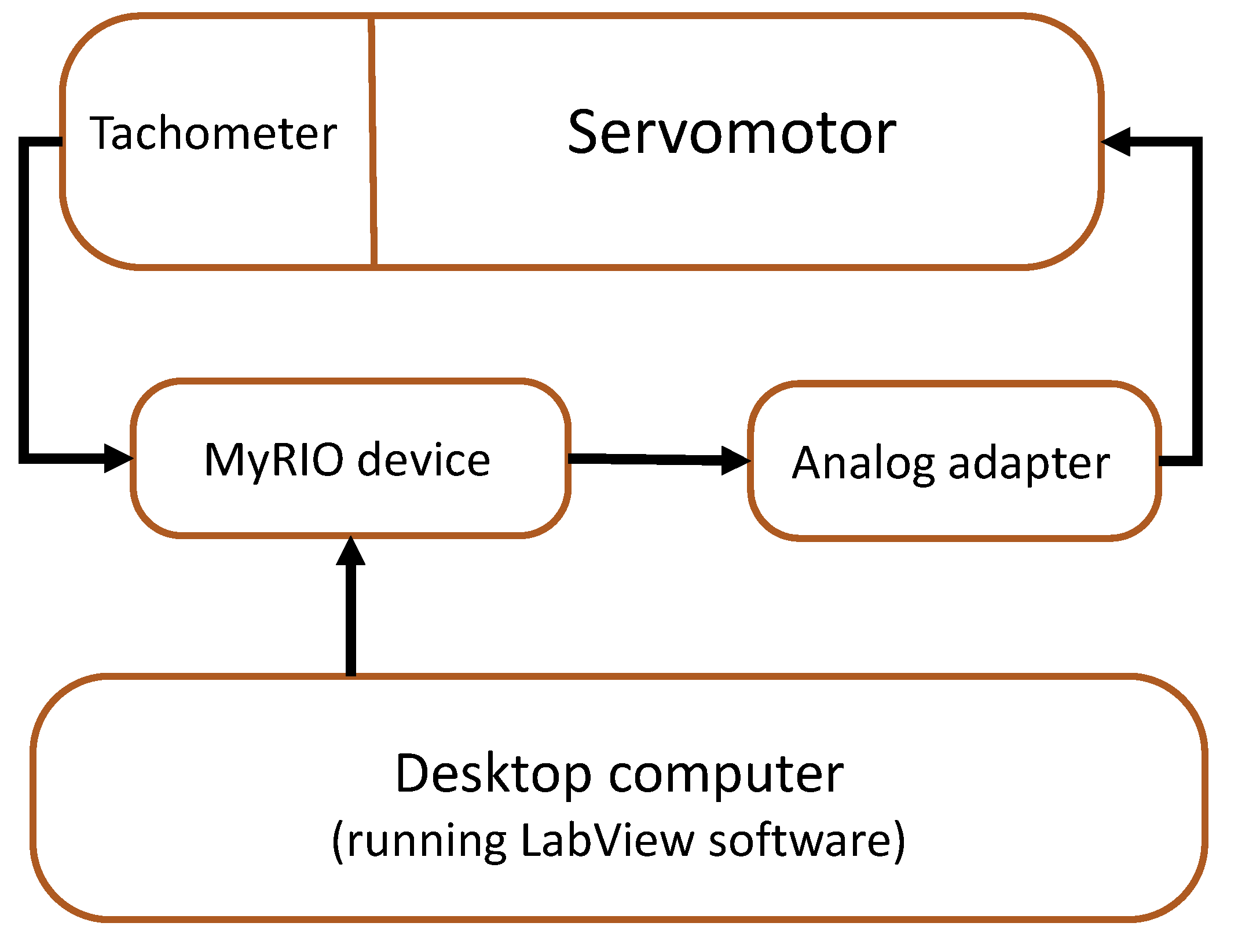
A rig for simulating the PTO formed by the servomotor, spring and sensors was oriented vertically and installed firmly to the carriage, Figure 8. A stainless steel spring was used for exerting the PTO restoring force and keeping the desired pretension. The electric motor was needed for simulating a realistic PTO damping force. The electric motor used (with an integrated tachometer) was a servomotor connected to the power unit and controlled by a MyRIO National Instruments device running an in-house developed model for controlling the motor. The motor was connected to an analogue adapter (power unit) and the MyRio device. A desktop computer was needed for running a LabView model that controlled the MyRio device and permitted to change PTO damping settings during the experiments (Figure 9).
The other three desktop computers were used for running the wavemaker, the Qualysis system and the Spike2 software for data acquisition, respectively.
A low-friction pulley was required to guide the mooring line from the bottom of the tank to the servomotor and the spring outside of the water, Figure 7b. This pulley was in-house manufactured and used during all tests in water.
2.9. Calibration and Uncertainty Analysis
The electric motor used as a damper was calibrated by performing a series of dry calibration tests before water tests. The motor was driven by using a wire and weights. For both clockwise and counterclockwise directions, different weights (one at a time) were attached to the wire and dropped. From the dropping time information, the speed and damping force exerted by the motor was calculated allowing the first calibration. Successively, an additional calibration method was implemented for fine-tuning and final characterization of the PTO force. The additional method related to targeting the right damping force using free oscillations tests. To obtain oscillations in the required range of frequencies, different combinations of springs and weights were used to test the PTO unit. The rig illustrated in Figure 10 was used for this purpose. Recursively, a weight was released from an initial offset and, one at a time, the time series of the oscillatory motion were logged. Successively, the classic second order differential equation, describing the motion of the damped harmonic oscillator, was solved at the end of each dry oscillation test for determining the damping coefficient value to assign to the oscillations obtained. The parameters of the damped harmonic model () were varied so to obtain a numerical solution matching the test results. Through these oscillation tests, the motor was characterized for a set of damping values. Once all calibration tests were performed, a look-up matrix was defined, which was later used for configuring the PTO during tests with the model in water.
Similarly, all other equipment was calibrated following best practices and performing several measurements for redundancy.
Following the guideline provided by [57], uncertainty values of all measurements can be calculated. In practice, five types of uncertainty values were calculated, namely: the standard uncertainty Type A, the standard uncertainty Type B, the standard uncertainty, the combined uncertainty and the expanded uncertainty.
The standard uncertainty, , is defined as:
where the and are respectively the Type A and Type B uncertainties values.
Type A uncertainty reflects repeatability of tests (due to statistical biases) and it is calculated by the equation:
where n is the number of repeated tests and is the standard deviation defined as:
where is the empirical reading associated with a particular test, and is the mean value obtained considering all the repeated measurements. During the experimental work, for calculating , five tests were repeated three times, and one test was repeated five times.
Type B uncertainty is not based on statistical methods and can be estimated by prior experience, calibration of equipment, manufacturers’ specifications and other relevant information.
Concerning the wave probes, load cells and laser sensor, a linear regression analysis, as reported by [58], can be used to calculate uncertainties. At first, the residuals, , that are the difference between the empirical data and the linear fit should be calculated:
The next step is the calculation of the sum of the square of residuals:
The Type B standard uncertainty is then calculated:
Regarding PTO damping, another approach was implemented for evaluating its uncertainty value, . This concerned specific calculations of the motor’s torque. The following torque relation was taken into account:
where the terms on the right side are respectively: desired motor torque, the torque due to motor inertia and torque due to friction.
The motor torque due to inertia is defined as:
where is the motor’s inertia constant provided by the manufacturer, and is the motor’s worm radius.
After substituting in Equation (30), the module of the load due to motor inertia was evaluated:
Taking into consideration the average heave velocity of the floater at resonance, the uncertainty of damping constant due to both effects of motor inertia and friction was combined as:
Successively, from the available information on uncertainties, the combined and expanded uncertainty values can be calculated. At first, the combined uncertainty concerning the measurement of power was assessed. Since the power was calculated from three inputs (indirect measurement), another approach was required for calculating its uncertainty. Considering that the power is defined as and, in the frequency-domain, , it can be defined as . The Data Reduction Equation for the combined uncertainty relative to power was set to be:
where the second term can be neglected because uncertainties of frequency , from repeated tests results, was found to be negligible. After substituting and into Equation (33), the combined uncertainty is given by:
Except for the uncertainty of the power measurement, for all other cases, the standard uncertainty, , was set equal to the combined uncertainty, .
Following the calculation of , the expanded uncertainty, , can be calculated for all measurements. For this purpose, a 95% confidence level was assumed, and, through the student’s distribution table, a coverage factor (for 3 repetitions) was identified. Given this coverage factor, is then calculated as for:
3. Results
For the demonstration of the novel numerical method, results relative to the PA described in Section 2.2 are provided. The theory and numerical formulations as explained in Section 2.3, Section 2.4, Section 2.5, Section 2.6 and Section 2.7 were used. Calculations were performed using an in-house developed MATLAB code and the NEMOH hydrodynamic code [51], but only for the calculation of the added mass, added damping and wave excitation forces coefficients.
3.1. Qualitative Assessment
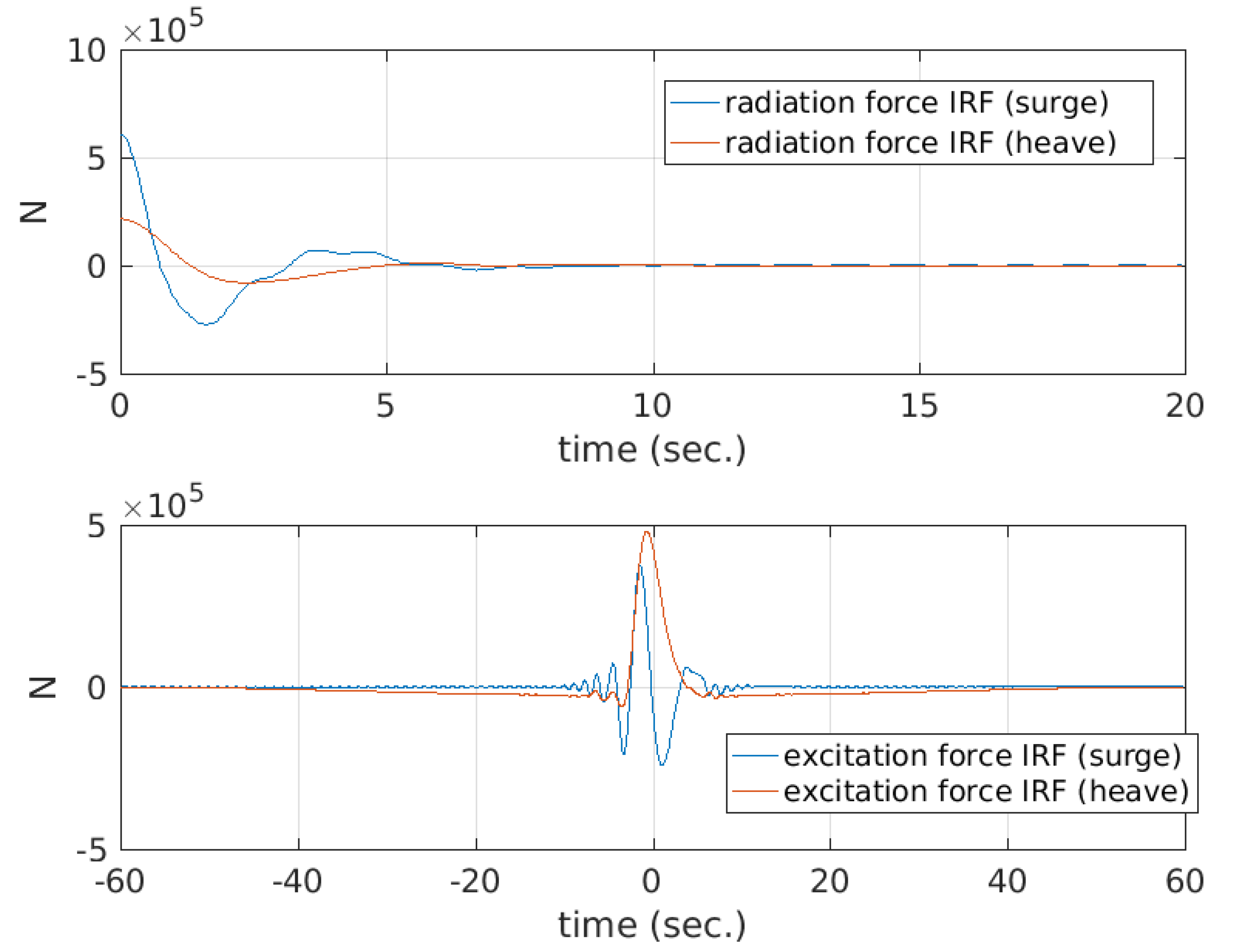
A qualitative assessment of the results obtained with the novel numerical method is presented first. Figure 11 reports the radiation and excitation force impulse response functions (IRF) for surge and heave directions. It can be observed for the PA geometry adopted that the radiation forces IRFs for heave and surge decay in about 20 s. Diversely, the IRFs for the excitation forces decay in ±60 s. In both cases, a correct decay occurs ensuring numerical stability.
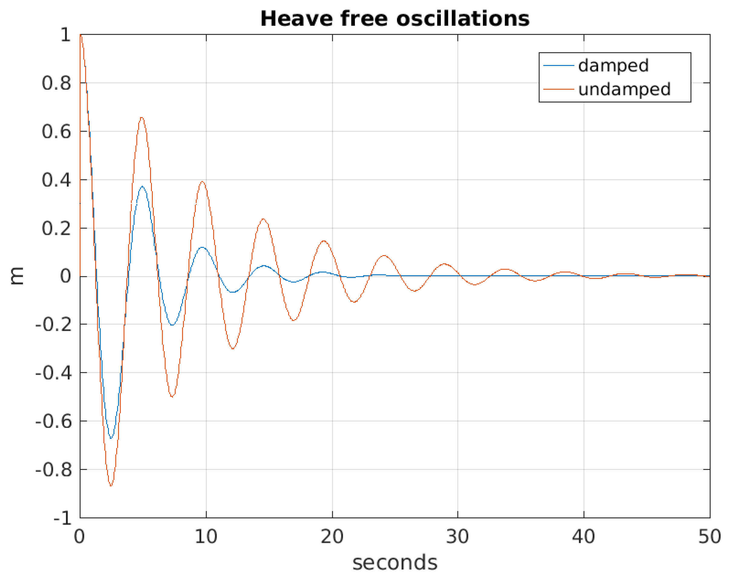
The numerical results of the surge and heave free-decay tests are illustrated in Figure 12 and Figure 13, respectively. It is observed that the numerical model correctly simulates, in qualitative terms, the PTO damping effect. In fact, for surge and heave motions—when the PTO damping condition is on—the motion is further decreased compared to the case when the PTO damping is off and the damping force is only due to hydrodynamic radiation damping.
When convolution integrals are used (IRWLO) in irregular sea simulations, the motion response, as expected, coincides with results obtained with the simplified direct wave loading option (DWLO), Figure 14. Note that, for this verification task, the wave drift forces are not included. Excluding wave drift forces was necessary, as, for the DWLO, it is not possible to include these forces. Thus, the IRWLO numerical simulation run for this comparison also had to be set with no wave drift forces.
3.2. Validation with Experimental Data
Afterwards, numerical results were compared with experimental data for validation. Where not explicitly mentioned, experimental results refer to the 1:33 model tested during the second repetition of the experiment. Two repetitions of the experiment were performed. During the second repetition, the experimental setup was improved, mostly for what concerns the PTO simulator unit. For this repetition uncertainty values were considerably reduced. Results for a corresponding 1:86 physical model [59] are also provided when available (Figure 15 and Figure 17).
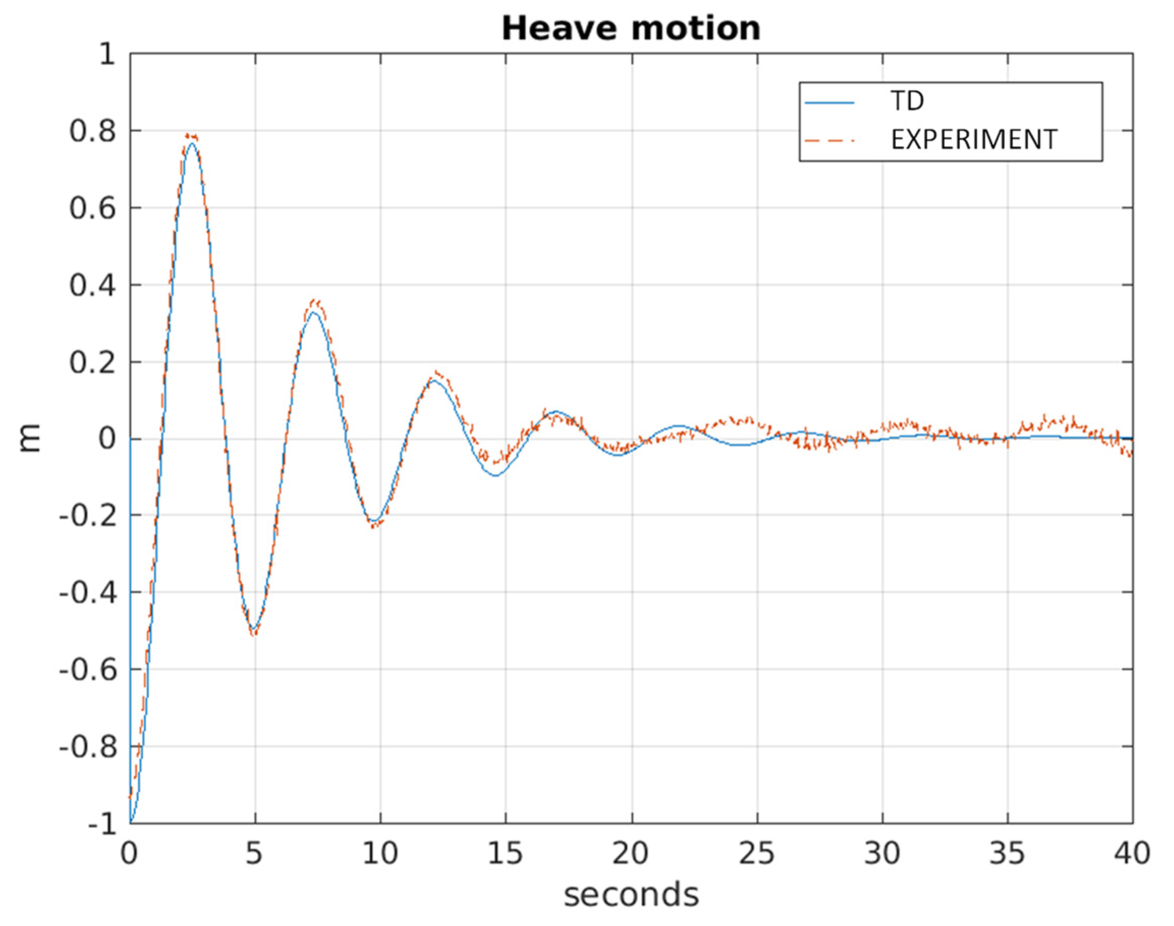
For surge and heave, free-decay tests results are illustrated in Figure 15 and Figure 16, respectively. For both directions of motion, results, in general, are in good agreement.
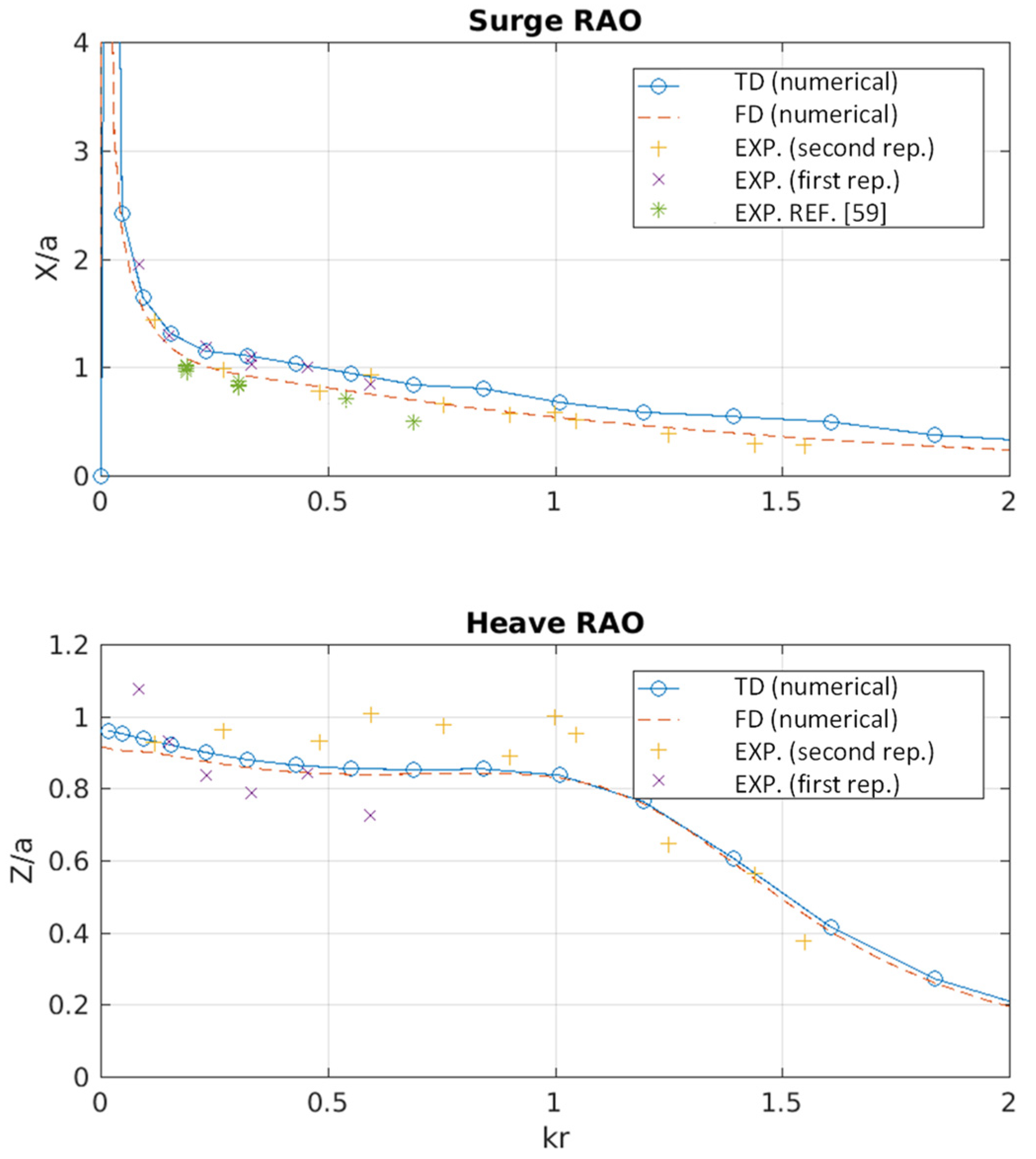
Regular wave test results were then compared to numerical simulation results in terms of Response Amplitude Operators (RAOs). To summarize the validation of regular sea tests graphically, each test result is represented by a point, which indicates the amplitude at the resonance condition following a sufficiently long interval. All results, in this case, are presented in the dimensionless form and plotted against the dimensionless wave number defined by the wavenumber and the floater radius . The main reason for this choice is that results in this form may be easily compared by others who carry out studies with a spherical floater of a different radius or use a different model scale. In general, numerical calculations predict well the 1:33 model-scale experimental measurements.
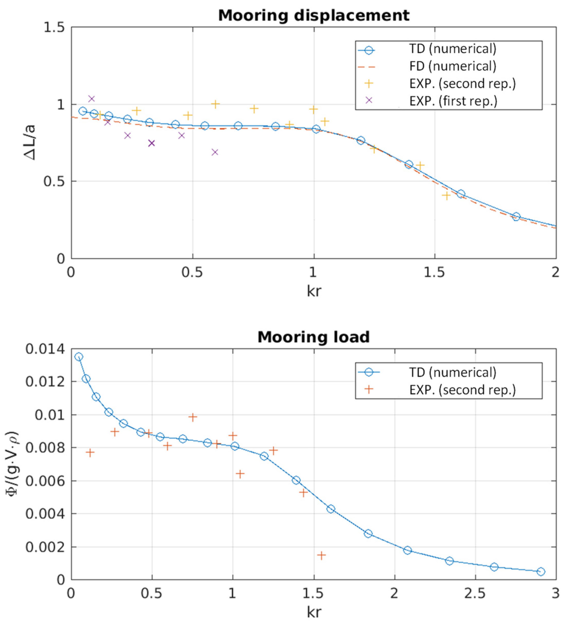
Together with RAOs curves (Figure 17), the mooring line displacement and the mooring load (Figure 18), as well as the power factor (Figure 19), are compared to the experimental results. Overall, all measurements are comparable to the numerical results with minor differences. The major dissimilarity between numerical and experimental quantities occurs for the dimensionless power factor assessment. This result may be because, in this case, the power is measured from a combination of measurements, and its related uncertainty value is higher.
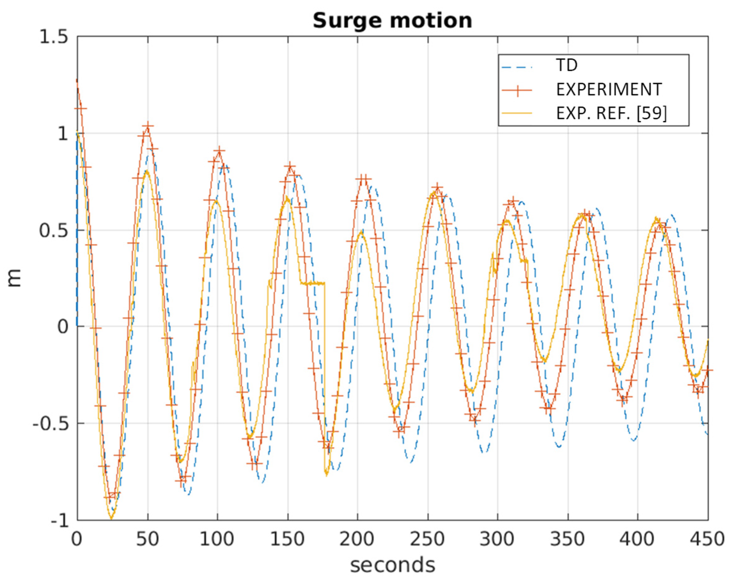
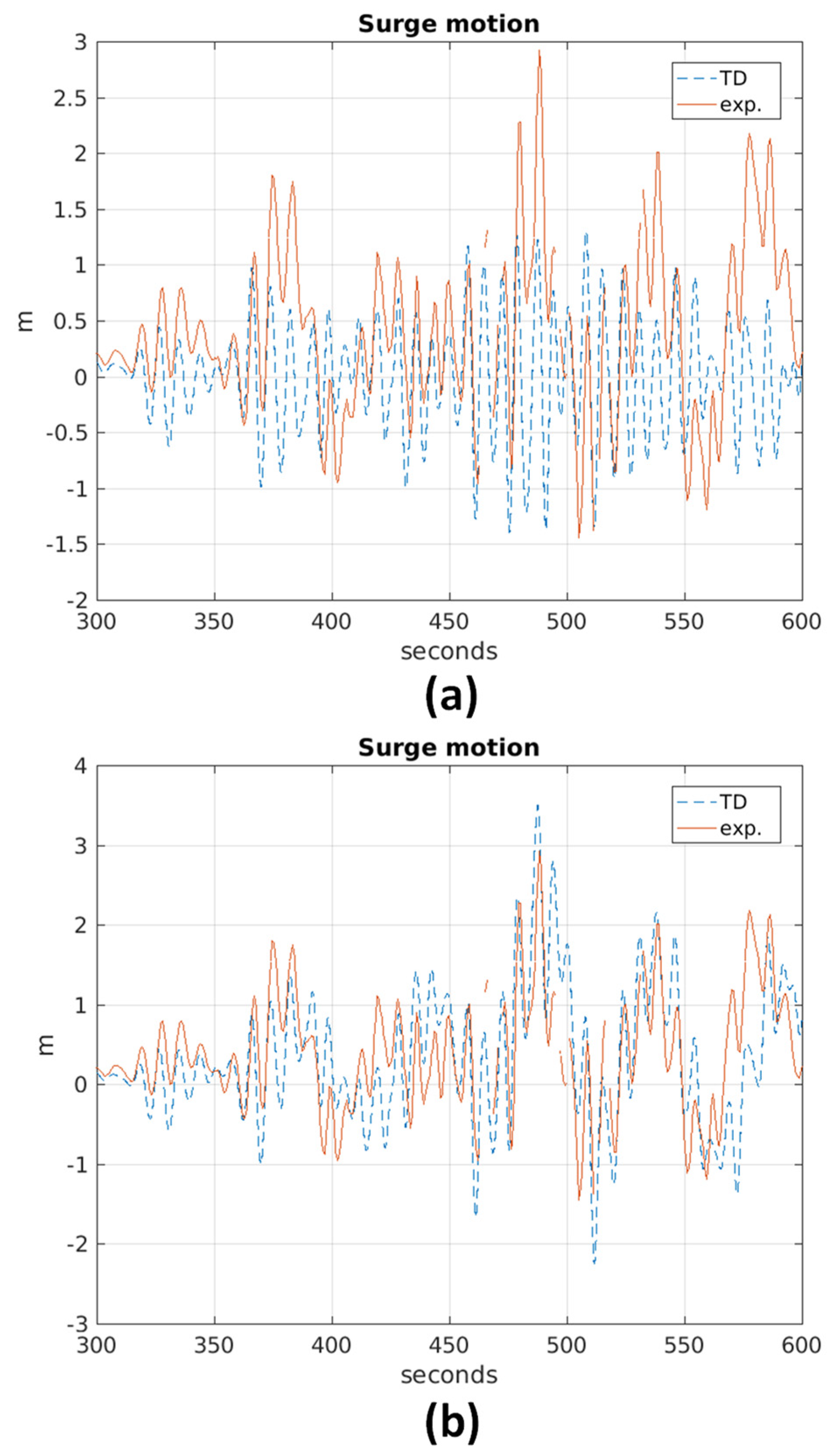
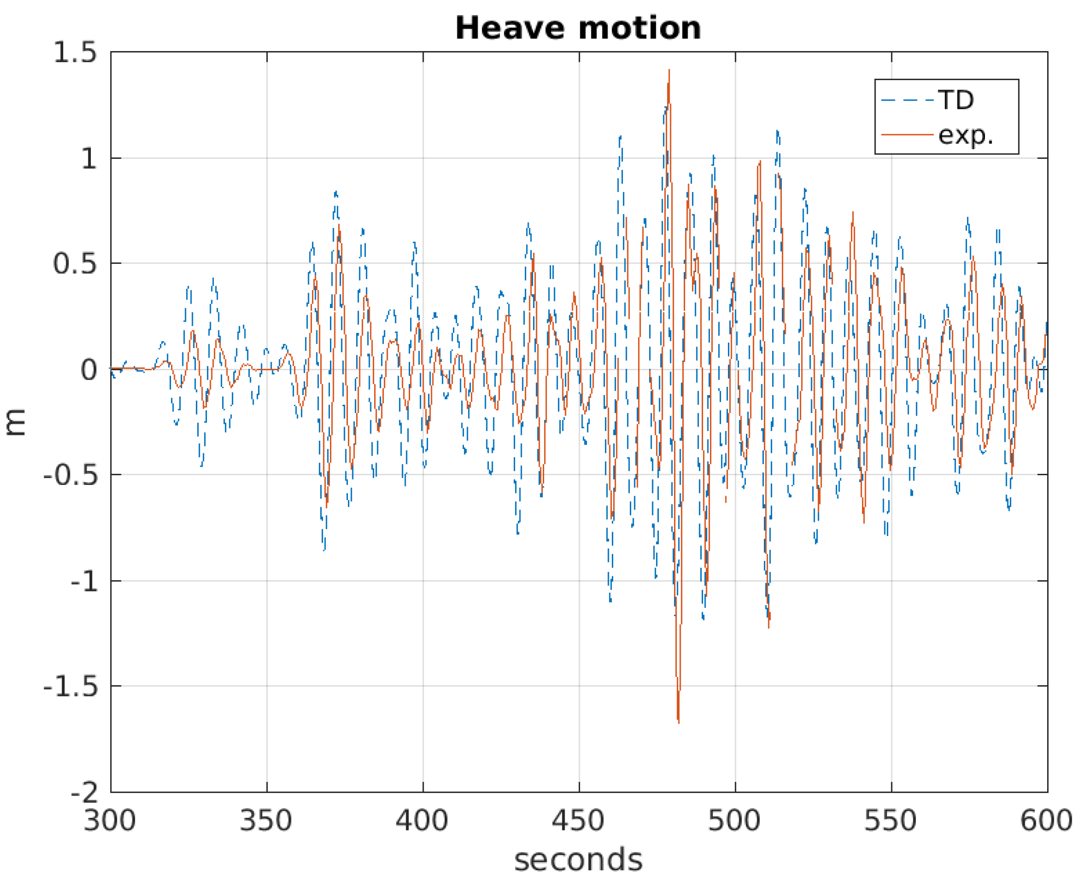
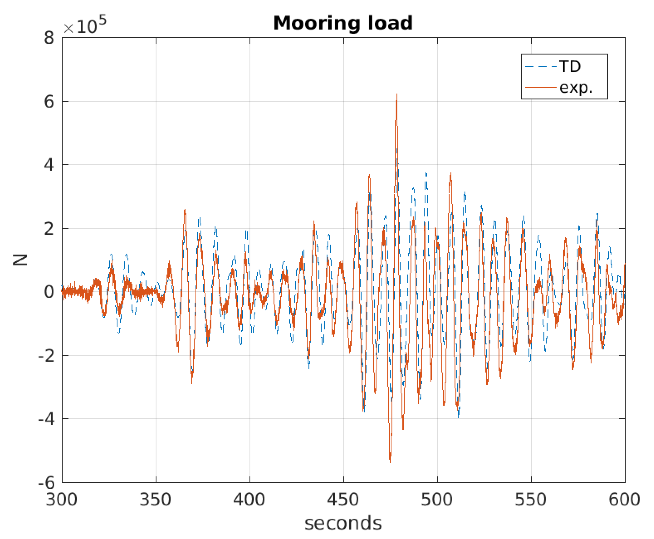
From the regular wave tests, it was possible to define the Cref coefficients (Table 3), which were then used in the irregular waves numerical simulations for including the drift forces. For what concerns irregular sea, results for the surge and heave response are illustrated for a specific sea state condition (Tp = 7.5 s, Hs = 2 m) in Figure 20 and Figure 21, respectively. The numerical surge motion, without drift forces, is far from the measured time series (Figure 20a). Differently, when drift forces are included, the numerical solution is well in agreement with the experimental measurement (Figure 20b). Similarly, the heave motion (Figure 21) and mooring load (Figure 22) are in good agreement with experimental estimated quantities.
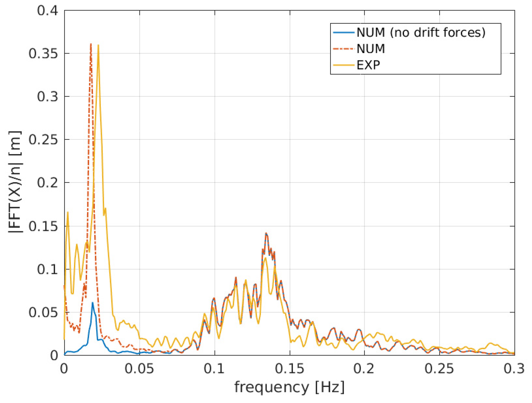
The Fast Fourier Transform (FFT) of the surge motion was calculated for further investigating the drift forces of the irregular sea state analyzed, Figure 23. As expected, the FFT, when no drift forces are considered, presents a significantly reduced peak at the low-frequency range of the spectrum. Peaks of the numerical result, including drift forces, and the experimental one are well comparable.
3.3. Uncertainty Analysis Results
For all experimental-related quantities, uncertainty values were calculated to understand the reliability of the experimental data used for numerical model validation, Table 4. For this assessment, regular waves tests data relative to two conditions are used ( and and ). Values of the Type A Uncertainty, Type B Uncertainty, Standard Uncertainty and the Expanded Uncertainty are reported. In general, uncertainty values are limited and increase with both the wave frequency and wave amplitude.
To check the experiment repeatability, several tests were repeated multiple times. For illustration, Table 5 reports the results of five tests run with the same input parameters ( and). As it can be observed, good repeatability was achieved during the experiment.
Although the repeatability was significantly good, the bias values, which can be obtained by the ratio of the expanded uncertainty and the mean values of measurements from repeated tests, are significant compared to direct and derived measurements, Table 6. The estimated bias in the case of motion and mooring displacements are up to about 24.3% of the measurement, and, for the power, it reaches about 64.5% of the indirect measurement. Experiments with a larger scale model may be required to increase overall accuracy.
3.4. Discussion
The proposed numerical method allows analyzing, together with the heave motion, the surge in the time domain. The method consents to calculate both the horizontal and vertical components of mooring loads, also taking into consideration the drift forces. This last is a clear advantage to the frequency domain approach, where the horizontal mooring restoring force can only be included by a significant linearization. Therefore, the proposed approach has the main advantage of enabling the inclusion of the drift forces for calculating the surge motion. As shown in Figure 20 (surge motion time series) and Figure 23 (Fast Fourier Transform analysis of the surge motion), the drift forces are critical in determining the surge motion. In addition, the proposed method has the advantage of allowing calculating the wave forces from a free-surface signal.
In spite of the previously described advantages, the proposed formulation presents some limitations that need to be mentioned. Specifically, both the frequency-domain and the time-domain formulations are valid for relatively limited displacements of the floating body (sphere) from the equilibrium position (x = 0, z = 0). In addition, these formulations are based on modelling the device taking as reference the mean free surface, i.e., it has to be pointed out that hydrodynamic coefficients obtained with the NEMOH code were calculated for the mean wetted floating body surface.
Furthermore, for the present study, the following simplifications were implemented:
- The mooring line is assumed to be inelastic. The only axial mooring displacement is due to the extension of the spring component. Depending on the material used, for a real installation, the mooring component elongation might be an important factor that needs to be investigated;
- Viscous forces are neglected. Note that for the typical size of wave power devices, operating in normal sea conditions, the viscous forces usually are significantly less than the first-order wave loads. The proposed methodology is not intended to be used for modelling the device for studying survivability of sea states conditions when, eventually, viscous effects are more significant. Moreover, to precisely estimate power absorption for relatively small devices at resonance conditions, viscous forces might be an important contribution;
- For simplicity, the mooring line is assumed to be attached to the center. In practice, this is not possible. However, due to the spherical shape considered and having assumed no viscous forces, it was possible to implement such simplification;
- The PTO system is modelled as a linear damping mechanism for which a single PTO damping coefficient can be set. The model, if appropriately extended, could be suitable for analyzing different, more complex types of PTO models, such as the hydraulic, phase-controlled systems, latching control or a combination of these.
4. Conclusions
The novel numerical method proposed permits the analysis of the dynamics of a PA device and its performance, including the effects of the PTO and mooring system. In this way, the structure response and its loads are predicted more realistically, as well as comprising drift forces and the surge direction of motion. The defined numerical method is based on frequency-domain calculations of hydrodynamic coefficients, using a BEM model, and on the time-domain method, where this last is formulated with the Cummins equation. The motion is solved for surge and heave, and the time-domain solution consents to include, into the analysis, transient hydrodynamic effects, thus allowing overcoming limitations of the frequency-domain-only approach. The proposed method enables the option of implementing, into the model, a defined free surface elevation signal as a wave loading input function. The latter feature can be needed for real-time applications, where the incoming wave can be measured at a certain distance upstream of the WEC. When developing a WEC, these extra capabilities are advantageous in comparison to conventional methods, where only resonance conditions can be assessed, and nonlinear effects cannot be included.
The numerical method developed was firstly verified and then validated with experimental data. Results obtained by the two options, related to the calculation of the wave forces, were compared for verification. Successively, numerical results were also compared to experimental data, which was acquired by an extended experimental campaign. The comparison was done for the free-decay, regular and irregular sea tests. Furthermore, a formal uncertainty analysis was carried out to quantify the accuracy of experimental measurements and derived quantities. In general, the numerical tool showed to predict, with reasonable accuracy, the dynamic behavior and performance of the studied WEC. For most cases, taking into account experiments’ uncertainty values, numerical predictions were within the expected ranges of results.
Author Contributions
Conceptualization, G.G. and S.D.; methodology, G.G.; formal analysis, G.G.; investigation, G.G.; resources, G.G.; data curation, G.G.; writing–original draft preparation, G.G.; writing–review and editing, P.R.-S., F.T.-P. and S.D.; visualization, G.G.; supervision, P.R.-S. and S.D.; project administration, P.R.-S. and F.T.-P.; funding acquisition, G.G., P.R.-S. and F.T.-P. All authors have read and agreed to the published version of the manuscript.
Funding
The work presented in this paper was possible thanks to a PhD scholarship provided by the University of Strathclyde. This publication was prepared, as well, thanks to funding from the project PORTOS—Ports Towards Energy Self-Sufficiency (EAPA 784/2018), co-financed by the Interreg Atlantic Area Program through the European Regional Development Fund.
Data Availability Statement
All important data is included in the manuscript.
Acknowledgments
The first author would like to acknowledge the Department of Naval, Architecture, Ocean and Marine Engineering of the University of Strathclyde, Scotland, including present and former academic, administrative and technical staff, for the aid and support provided during his PhD.
Conflicts of Interest
The authors declare no conflict of interest.
References
- Gunn, K.; Stock-Williams, C. Quantifying the global wave power resource. Renew. Energy 2012, 44, 296–304. [Google Scholar] [CrossRef]
- Giannini, G. Modelling and Feasibility Study on Using Tidal Power with an Energy Storage Utility for Residential Needs. Inventions 2019, 4, 11. [Google Scholar] [CrossRef] [Green Version]
- Todeschini, G. Review of Tidal Lagoon Technology and Opportunities for Integration within the UK Energy System. Inventions 2017, 2, 14. [Google Scholar] [CrossRef] [Green Version]
- Charlier, R.H.; Justus, J.R. (Eds.) Chapter 5 waves. In Elsevier Oceanography Series; Elsevier: Amsterdam, The Netherlands, 1993; pp. 105–185. ISBN 0422-9894. [Google Scholar] [CrossRef]
- Heath, T.V. A review of oscillating water columns. Philos. Trans. R. Soc. A Math. Phys. Eng. Sci. 2012, 370, 235–245. [Google Scholar] [CrossRef] [Green Version]
- Portillo, J.; Collins, K.; Gomes, R.; Henriques, J.; Gato, L.; Howey, B.; Hann, M.; Greaves, D.; Falcão, A. Wave energy converter physical model design and testing: The case of floating oscillating-water-columns. Appl. Energy 2020, 278, 115638. [Google Scholar] [CrossRef]
- Giannini, G.; López, M.; Ramos, V.; Rodríguez, C.A.; Rosa-Santos, P.; Taveira-Pinto, F. Geometry assessment of a sloped type wave energy converter. Renew. Energy 2021, 171, 672–686. [Google Scholar] [CrossRef]
- Coiro, D.P.; Troise, G.; Calise, G.; Bizzarrini, N. Wave energy conversion through a point pivoted absorber: Numerical and experimental tests on a scaled model. Renew. Energy 2016, 87, 317–325. [Google Scholar] [CrossRef]
- Rosa-Santos, P.; Taveira-Pinto, F.; Teixeira, L.; Ribeiro, J. CECO wave energy converter: Experimental proof of concept. J. Renew. Sustain. Energy 2015, 7, 061704. [Google Scholar] [CrossRef]
- Sarkar, D.; Doherty, K.; Dias, F. The modular concept of the Oscillating Wave Surge Converter. Renew. Energy 2016, 85, 484–497. [Google Scholar] [CrossRef]
- Salter, S.H. The Solo Duck. 1982. Available online: http://www.homepages.ed.ac.uk/v1ewaveg/0-Archive/EWPP%20archive/1982%20EWPP%20The%20Solo%20Duck.pdf (accessed on 1 December 2019).
- Kofoed, J.P.; Frigaard, P.; Friis-Madsen, E.; Sørensen, H.C. Prototype testing of the wave energy converter wave dragon. Renew. Energy 2006, 31, 181–189. [Google Scholar] [CrossRef] [Green Version]
- Margheritini, L.; Vicinanza, D.; Frigaard, P. SSG wave energy converter: Design, reliability and hydraulic performance of an innovative overtopping device. Renew. Energy 2009, 34, 1371–1380. [Google Scholar] [CrossRef]
- Fernandez, H.; Iglesias, G.; Carballo, R.; Castro, A.; Fraguela, J.; Taveira-Pinto, F.; Sanchez, M. The new wave energy converter WaveCat: Concept and laboratory tests. Mar. Struct. 2012, 29, 58–70. [Google Scholar] [CrossRef]
- Faizal, M.; Ahmed, M.R.; Lee, Y.-H. A Design Outline for Floating Point Absorber Wave Energy Converters. Adv. Mech. Eng. 2014, 6. [Google Scholar] [CrossRef] [Green Version]
- Kolios, A.; Di Maio, L.F.; Wang, L.; Cui, L.; Sheng, Q. Reliability assessment of point-absorber wave energy converters. Ocean Eng. 2018, 163, 40–50. [Google Scholar] [CrossRef]
- Agyekum, E.; PraveenKumar, S.; Eliseev, A.; Velkin, V. Design and Construction of a Novel Simple and Low-Cost Test Bench Point-Absorber Wave Energy Converter Emulator System. Inventions 2021, 6, 20. [Google Scholar] [CrossRef]
- Falcão, A.F.D.O. Wave energy utilization: A review of the technologies. Renew. Sustain. Energy Rev. 2010, 14, 899–918. [Google Scholar] [CrossRef]
- Carnegie Clean Energy. CETO. Available online: https://www.carnegiece.com/technology/ (accessed on 15 June 2020).
- Ocean Power Technology (OPT). Available online: https://oceanpowertechnologies.com/ (accessed on 25 September 2021).
- Osawa, H.; Washio, Y.; Ogata, T.; Tsuritani, Y.; Nagata, Y. The Offshore Floating Type Wave Power Device “Mighty Whale” Open Sea TestsPerformance of The Prototype. In The Twelfth International Offshore and Polar Engineering Conference; International Society of Offshore and Polar Engineers: Kitakyushu, Japan, 2002; p. 6. [Google Scholar]
- Babarit, A.; Clément, A.; Ruer, J.; Tartivel, C. SEAREV: A Fully Integrated Wave Energy Converter; Ecole Centrale de Nantes: Nantes, France, 2006. [Google Scholar]
- Mattiazzo, G. State of the Art and Perspectives of Wave Energy in the Mediterranean Sea: Backstage of ISWEC. Front. Energy Res. 2019, 7, 114. [Google Scholar] [CrossRef] [Green Version]
- Boren, B.C.; Batten, B.A.; Paasch, R.K. Active control of a vertical axis pendulum wave energy converter. In Proceedings of the 2014 American Control Conference, Portland, OR, USA, 21 July 2014; ISBN 2378-5861. [Google Scholar] [CrossRef]
- AW-Energy. Available online: https://aw-energy.com/waveroller/ (accessed on 16 June 2020).
- Henry, A.; Power, U.A.; Doherty, K.; Cameron, L.; Doherty, R.; Whittaker, T. Advances in the Design of the Oyster Wave Energy Converter; Marine Renewable & Offshore Wind Energy, RINA HQ: London, UK, 2010. [Google Scholar]
- Johanning, L.; Smith, G.H.; Wolfram, J. Mooring design approach for wave energy converters. Proc. Inst. Mech. Eng. Part M J. Eng. Marit. Environ. 2006, 220, 159–174. [Google Scholar] [CrossRef]
- Barltrop, N.D.P. Floating Structures: A Guide for Design and Analysis; Oilfield Publications: Ledbury, UK, 1998; Volume 1–2. [Google Scholar]
- Rahman, A.; Farrok, O.; Islam, R.; Xu, W. Recent Progress in Electrical Generators for Oceanic Wave Energy Conversion. IEEE Access 2020, 8, 138595–138615. [Google Scholar] [CrossRef]
- Farrok, O.; Islam, R.; Sheikh, R.I.; Guo, Y.; Zhu, J.; Lei, G. Oceanic Wave Energy Conversion by a Novel Permanent Magnet Linear Generator Capable of Preventing Demagnetization. IEEE Trans. Ind. Appl. 2018, 54, 6005–6014. [Google Scholar] [CrossRef]
- Kiran, M.R.; Farrok, O.; Mamun, A.-A.; Islam, R.; Xu, W. Progress in Piezoelectric Material Based Oceanic Wave Energy Conversion Technology. IEEE Access 2020, 8, 146428–146449. [Google Scholar] [CrossRef]
- Molla, S.; Farrok, O.; Rahman, A.; Bashir, S.; Islam, R.; Kouzani, A.Z.; Mahmud, M.A.P. Increase in Volumetric Electrical Power Density of a Linear Generator by Winding Optimization for Wave Energy Extraction. IEEE Access 2020, 8, 181605–181618. [Google Scholar] [CrossRef]
- Beatty, S.J.; Hall, M.; Buckham, B.J.; Wild, P.; Bocking, B. Experimental and numerical comparisons of self-reacting point absorber wave energy converters in regular waves. Ocean Eng. 2015, 104, 370–386. [Google Scholar] [CrossRef]
- Shadman, M.; Avalos, G.O.G.; Estefen, S.F. On the power performance of a wave energy converter with a direct mechanical drive power take-off system controlled by latching. Renew. Energy 2021, 169, 157–177. [Google Scholar] [CrossRef]
- Wu, J.; Yao, Y.; Zhou, L.; Göteman, M. Real-time latching control strategies for the solo Duck wave energy converter in irregular waves. Appl. Energy 2018, 222, 717–728. [Google Scholar] [CrossRef]
- Cruz, J.M.B.P.; Sarmento, A.J.N.A. Time domain simulations on a single point moored submerged sphere of variable radius. In Proceedings of the 24th International Conference on Offshore Mechanics and Arctic Engineering, Halkidiki, Greece, 12–17 June 2005. [Google Scholar]
- Vicente, P.V.; Falcão, A.F.O.; Justino, P.A.P. Nonlinear dynamics of a tighly moored point-absorber wave energy converter. Ocean Eng. 2013, 59, 20–36. [Google Scholar] [CrossRef] [Green Version]
- Mavrakos, S.A.; Katsaounis, M.G. Parametric evaluation of the performance characteristics of tight moored wave energy converters. In Proceedings of the 24th International Conference on Offshore Mechanics and Arctic Engineering, Halkidiki, Greece, 12–17 June 2005. [Google Scholar]
- Mavrakos, S.A.; Katsaounis, G.M.; Apostolidis, M.S. Effects of floaters’ geometry on the performance characteristics of a tighly moored wave energy converters. In Proceedings of the ASME 2009 28th International Conference on Ocean, Offshore and Arctic Engineering, Honolulu, HI, USA, 31 May–5 June 2009. [Google Scholar]
- Spanos, P.D.; Arena, F.; Richichi, A.; Malara, G. Efficient Dynamic Analysis of a Nonlinear Wave Energy Harvester Model. J. Offshore Mech. Arct. Eng. 2016, 138, 041901. [Google Scholar] [CrossRef]
- Giannini, G.; Temiz, I.; Rosa-Santos, P.; Shahroozi, Z.; Ramos, V.; Göteman, M.; Engström, J.; Day, S.; Taveira-Pinto, F. Wave Energy Converter Power Take-Off System Scaling and Physical Modelling. J. Mar. Sci. Eng. 2020, 8, 632. [Google Scholar] [CrossRef]
- Hann, M.; Greaves, D.; Raby, A. Snatch loading of a single taut moored floating wave energy converter due to focused wave groups. Ocean Eng. 2015, 96, 258–271. [Google Scholar] [CrossRef] [Green Version]
- Orszaghova, J.; Rafiee, A.; Wolgamot, H.; Draper, S.; Taylor, P.H. Experimental Study of Extreme Responses of a Point Absorber Wave Energy Converter. In Proceedings of the 20th Australasian Fluid Mechanics Conference, Perth, Australia, 5–8 December 2016. [Google Scholar]
- Radhakrishnan, S.; Datla, R.; Hires, R.I. Theoretical and experimental analysis of tethered buoy instability in gravity waves. Ocean Eng. 2007, 34, 261–274. [Google Scholar] [CrossRef]
- Gunn, D.F.; Rudman, M.; Cohen, R. Wave interaction with a tethered buoy: SPH simulation and experimental validation. Ocean Eng. 2018, 156, 306–317. [Google Scholar] [CrossRef]
- Wang, W.; Wu, M.; Palm, J.; Eskilsson, C. Estimation of numerical uncertainty in CFD simulations of a passively controlled wave energy converter. J. Eng. Marit. Environ. 2018, 232, 71–84. [Google Scholar]
- Ding, B.; Souza, L.; Silva, P.; Sergiienko, N.; Meng, F.; Piper, J.; Bennetts, L.; Wagner, M.; Cazzolato, B.; Arjomandi, M. Study of fully submerged point absorber wave energy converter—Modelling, simulation and scaled experiment. In Proceedings of the 32nd International Workshop on Water Waves and Floating Bodies, Dalian, China, 23–26 April 2017. [Google Scholar]
- Cummins, W.E. The impulse response function and ship motions. In Proceedings of the Report 1661 of the, Symposium on Ship Theory at the Institut für Schiffbau der Universität, Hamburg, Germany, 25–27 January 1962. [Google Scholar]
- Ogilvie, T.F. Recent Progress toward the Understanding and Prediction of Ship Motions. 1964. Available online: https://repository.tudelft.nl/ (accessed on 24 June 2021).
- Babarit, A. Nemoh—Website. 2014. Available online: https://lheea.ec-nantes.fr/research-impact/software-and-patents/nemoh-presentation (accessed on 24 June 2021).
- Babarit, A.; Delhommeau, G. Theoretical and numerical aspects of the open source BEM solver NEMOH. In Proceedings of the 11th European Wave and Tidal Energy Conference (EWTEC2015), Nantes, France, 6–11 September 2015. [Google Scholar]
- Journee, J.M.J.; Massie, W.W. Offshore Hydromechanics. Delf University of Technology, Netherlands. 2001. Available online: https://ocw.tudelft.nl/wp-content/uploads/OffshoreHydromechanics_Journee_Massie.pdf (accessed on 10 October 2020).
- Falnes, J. Ocean Waves and Oscillating Systems; Cambridge University Press: Cambridge, UK, 2002. [Google Scholar]
- Hsu, F.H.; Blenkarn, K.A. Analysis of Peak Mooring Forces Caused by Slow Vessel Drift Oscillations in Random Seas. Soc. Pet. Eng. J. 1972, 12, 329–344. [Google Scholar] [CrossRef]
- Remery, G.F.M.; Hermans, A.J. The Slow Drift Oscillations of a Moored Object in Random Seas. Soc. Pet. Eng. J. 1972, 12, 191–198. [Google Scholar] [CrossRef]
- UoStrath—Kelvin Hydrodynamics Laboratory (Formerly Acre Road Wave and Tow Tank). Available online: http://130.159.19.247/engineering/navalarchitectureoceanmarineengineering/workingwithbusinessorganisations/ourfacilities/kelvinhydrodynamicslaboratory/ (accessed on 10 October 2021).
- ITTC. Uncertainty Analysis for a Wave Energy Converter. Part of the ITTC Quality System Manual—Recommended Procedures and Guidelines. 2017. Available online: https://www.ittc.info/media/8135/75-02-07-0312.pdf (accessed on 10 October 2021).
- ITTC. Uncertainty Analysis, Instrument Calibration. In Proceedings of the ITTC Quality System Manual Recommended Procedures and Guidelines. 2017. Available online: https://www.ittc.info/media/7979/75-01-03-01.pdf (accessed on 10 October 2021).
- Giannini, G. Mooring Analysis and Design for Wave Energy Converters; University of Strathclyde Online Library: Glasgow, UK, 2018. [Google Scholar]
Figure 1.
Types of offshore wave energy converters and examples.

Figure 2.
Examples of point absorbers: (a) the Seabased, (b) the CETO, (c) the CorPower PA and (d) the BOLT Lifesaver WEC.
Figure 2.
Examples of point absorbers: (a) the Seabased, (b) the CETO, (c) the CorPower PA and (d) the BOLT Lifesaver WEC.

Figure 3.
Experimental setups used in hydrodynamic experiments of point absorbers. (a,c–f) are devices with a surface-located floater and (b,g) are devices with a fully submerged floater.
Figure 3.
Experimental setups used in hydrodynamic experiments of point absorbers. (a,c–f) are devices with a surface-located floater and (b,g) are devices with a fully submerged floater.

Figure 4.
Point absorber model considered. In (a) the geometry and (b) the mesh (200 panels), used for the numerical model, are illustrated, respectively.
Figure 4.
Point absorber model considered. In (a) the geometry and (b) the mesh (200 panels), used for the numerical model, are illustrated, respectively.

Figure 5.
A mechanical analogy of the considered system for defining the numerical approximation related to the horizontal mooring restoring force component.
Figure 5.
A mechanical analogy of the considered system for defining the numerical approximation related to the horizontal mooring restoring force component.

Figure 6.
Experiment setup: (a) side view, (b) top view and (c) approximate position of the Qualysis cameras.
Figure 6.
Experiment setup: (a) side view, (b) top view and (c) approximate position of the Qualysis cameras.

Figure 7.
Photos of experiments: (a) carriage, mooring line and floater location, (b) low friction pulley, (c) floater with reflectors for motion capturing during regular waves testing.
Figure 7.
Photos of experiments: (a) carriage, mooring line and floater location, (b) low friction pulley, (c) floater with reflectors for motion capturing during regular waves testing.

Figure 8.
PTO rig: (a) electric servomotor, (b) laser sensor and spring and (c) load cell.

Figure 9.
Scheme of connections for PTO motor control.

Figure 10.
PTO calibration rig.

Figure 11.
Radiation and excitation force impulse response functions for surge and heave directions (numerical).
Figure 11.
Radiation and excitation force impulse response functions for surge and heave directions (numerical).

Figure 12.
Damped and undamped surge free-decay time series (numerical).

Figure 13.
Damped and undamped heave free-decay time series (numerical).

Figure 14.
System response in the irregular sea (Tp = 10 s, Hs = 2 m) given by the two options for estimating time-dependent wave loads (numerical).
Figure 14.
System response in the irregular sea (Tp = 10 s, Hs = 2 m) given by the two options for estimating time-dependent wave loads (numerical).

Figure 15.
Numerical and experimental results for surge free-decay tests.

Figure 16.
Numerical and experimental results for heave free-decay tests.

Figure 17.
Surge and heave response amplitude operators (RAO) validation (numerical and experimental).
Figure 17.
Surge and heave response amplitude operators (RAO) validation (numerical and experimental).

Figure 18.
Mooring displacement and mooring load validation (numerical and experimental).

Figure 19.
Dimensionless power factor results for regular wave tests (numerical and experimental).

Figure 20.
Surge response numerical and experimental results for an irregular sea state (Tp = 7.5 s, Hs = 2.0 m). Numerical results for the simulations are without (a) and with (b) drift forces.
Figure 20.
Surge response numerical and experimental results for an irregular sea state (Tp = 7.5 s, Hs = 2.0 m). Numerical results for the simulations are without (a) and with (b) drift forces.

Figure 21.
Heave response numerical and experimental results for an irregular sea state (Tp = 7.5 s, Hs = 2.0 m).
Figure 21.
Heave response numerical and experimental results for an irregular sea state (Tp = 7.5 s, Hs = 2.0 m).

Figure 22.
Mooring load numerical and experimental results for an irregular sea state (Tp = 7.5 s, Hs = 2.0 m).
Figure 22.
Mooring load numerical and experimental results for an irregular sea state (Tp = 7.5 s, Hs = 2.0 m).

Figure 23.
Spectral analysis of surge motion time series (numerical and experimental) results (Tp = 7.5 s, Hs = 2.0 m).
Figure 23.
Spectral analysis of surge motion time series (numerical and experimental) results (Tp = 7.5 s, Hs = 2.0 m).


Table 1.
Instruments and measurements.
| Instrument | Measurement | Range | Unit |
|---|---|---|---|
| Motion capture system | Floater displacement | 0–500 | mm |
| Standard wave probe | Free-surface elevation | 0–150 | mm |
| Sonic wave probe | Free-surface elevation upstream | 0–150 | Mm |
| Load cell | Mooring tension | 0–50 | N |
| Laser sensor | Mooring line displacement | 0–350 | Mm |
| Motor tachometer | Mooring line displacement | 0–350 | mm |
Table 2.
Physical model parameters and real scale corresponding quantities.
| Parameter | Model Scale (1:33) | Real Scale (1:1) | Unit |
|---|---|---|---|
| Floater radius | m | ||
| Floater mass | kg | ||
| Water depth | m | ||
| Mooring line length | m | ||
| Spring stiffness | N/m | ||
| Cpto damping | kg/s | ||
| Mooring pretension | N |
Table 3.
Reflection coefficients from regular wave tests for the calculation of drift forces during irregular sea numerical tests.
Table 3.
Reflection coefficients from regular wave tests for the calculation of drift forces during irregular sea numerical tests.
| ω (rad/s) | 0.40 | 0.46 | 0.53 | 0.59 | 0.66 | 0.72 | 0.79 | 0.86 | 0.92 | 0.99 | 1.05 | 1.12 | 1.18 | 1.25 | 1.31 |
| Crefl | 0.10 | 0.11 | 0.15 | 0.25 | 0.30 | 0.35 | 0.40 | 0.45 | 0.45 | 0.50 | 0.50 | 0.55 | 0.60 | 0.70 | 1.00 |
Table 4.
Uncertainty analysis results.
| Units | ||||||||||||
|---|---|---|---|---|---|---|---|---|---|---|---|---|
| Waves Characteristics | Ampl. | (mm) | 30 | 30 | 60 | 30 | 30 | 60 | 30 | 30 | 60 | |
| Freq. | (rad/s) | 2.3 | 6.6 | 6.6 | 2.3 | 6.6 | 6.6 | 2.3 | 6.6 | 6.6 | ||
| Heave | Ampl. (mm) | 0.763 | 1.545 | 2.39 | 0.8 | 1.105 | 1.74 | 2.52 | 4.753 | 7.482 | 10.838 | |
| Freq. (rad/s) | 0.002 | 0.008 | 0.004 | 0.002 | 0.008 | 0.004 | 0.008 | 0.036 | 0.018 | |||
| Surge | Ampl. (mm) | 0.66 | 0.123 | 0.31 | 0.8 | 1.037 | 0.809 | 0.858 | 4.46 | 3.481 | 3.69 | |
| Freq. (rad/s) | 0.005 | 0.017 | 0.003 | 0.005 | 0.017 | 0.003 | 0.021 | 0.073 | 0.013 | |||
| Direct meas. | Wave probe | Ampl. (mm) | 0.891 | 0.341 | 2.099 | 0.7 | 1.133 | 0.779 | 2.213 | 4.873 | 3.349 | 9.516 |
| Freq. (rad/s) | 0.002 | 0.004 | 0.003 | 0.002 | 0.004 | 0.003 | 0.009 | 0.016 | 0.013 | |||
| Load | Ampl. (N) | 0.056 | 0.119 | 0.138 | 0.015 | 0.058 | 0.12 | 0.138 | 0.25 | 0.517 | 0.595 | |
| Freq. (rad/s) | 0.001 | 0.007 | 0.004 | 0.001 | 0.007 | 0.004 | 0.006 | 0.031 | 0.016 | |||
| Displacement | Ampl. (mm) | 0.822 | 1.73 | 2.176 | 0.85 | 1.183 | 1.927 | 2.336 | 5.085 | 8.288 | 10.044 | |
| Freq. (rad/s) | 0.002 | 0.006 | 0.003 | 0.002 | 0.006 | 0.003 | 0.007 | 0.028 | 0.011 | |||
| Sim. of PTO | PTO damping | (kg/s) | 1.473 | 1.473 | 1.473 | 1.473 | NA | NA | NA | |||
| Spring stiffness | (N/m) | 13.212 | 13.212 | 13.212 | 13.212 | NA | NA | NA | ||||
| Mass of floater | (kg) | 0.005 | 0.005 | 0.005 | 0.005 | NA | NA | NA | ||||
| Fixed param. | Radius of floater | (mm) | 0.8 | 0.8 | 0.8 | 0.8 | NA | NA | NA | |||
| Length of line | (mm) | 6 | 6 | 6 | 6 | NA | NA | NA | ||||
| Pretension | (N) | 0.056 | 0.119 | 0.138 | 0.015 | 0.058 | 0.12 | 0.183 | 0.25 | 0.517 | 0.786 | |
| Indirect meas. | Power | (W) | 0.03 | 0.328 | 1.221 |
Table 5.
Regular waves tests (α = 30 mm and ω = 4.6 rad/s) repeated 5 times.
| Test No.: | 12 | 25 | 35 | 38 | 53 | ||
|---|---|---|---|---|---|---|---|
| Heave | Ampl. (mm) | 29.527 | 28.476 | 30.847 | 30.782 | 31.258 | 0.728 |
| Freq. (rad/s) | 4.585 | 4.608 | 4.588 | 4.58 | 4.594 | 0.007 | |
| Surge | Ampl. (mm) | 26.168 | 23.079 | 24.98 | 26.281 | 25.295 | 0.816 |
| Freq. (rad/s) | 4.643 | 4.524 | 4.589 | 4.55 | 4.592 | 0.029 | |
| Wave probe | Ampl. (mm) | 33.027 | 34.506 | 34.02 | 32.872 | 33.884 | 0.438 |
| Freq. (rad/s) | 4.596 | 4.609 | 4.594 | 4.592 | 4.594 | 0.004 | |
| Load | Ampl. (N) | 2.156 | 2.067 | 2.248 | 2.249 | 2.278 | 0.055 |
| Freq. (rad/s) | 4.588 | 4.604 | 4.589 | 4.578 | 4.594 | 0.006 | |
| Displacement | Ampl. (mm) | 29.732 | 28.305 | 30.742 | 30.927 | 31.253 | 0.758 |
| Freq. (rad/s) | 4.587 | 4.603 | 4.589 | 4.578 | 4.594 | 0.006 |
Table 6.
Total bias (in percentage) related to the physical model for the repeated tests.
| Quantity | Total bias (±%) | |
|---|---|---|
| Heave | ampl. | 21.41 |
| phase | 0.55 | |
| Surge | ampl. | 20.68 |
| phase | 1.11 | |
| Wave probe | ampl. | 10.76 |
| phase | 0.25 | |
| Load | ampl. | 20.36 |
| phase | 0.47 | |
| Displacement | ampl. | 24.27 |
| phase | 0.42 | |
| Power | ampl. | 64.45 |
Publisher’s Note: MDPI stays neutral with regard to jurisdictional claims in published maps and institutional affiliations. |
© 2021 by the authors. Licensee MDPI, Basel, Switzerland. This article is an open access article distributed under the terms and conditions of the Creative Commons Attribution (CC BY) license (https://creativecommons.org/licenses/by/4.0/).
Share and Cite
MDPI and ACS Style
Giannini, G.; Day, S.; Rosa-Santos, P.; Taveira-Pinto, F. A Novel 2-D Point Absorber Numerical Modelling Method. Inventions 2021, 6, 75. https://doi.org/10.3390/inventions6040075
AMA Style
Giannini G, Day S, Rosa-Santos P, Taveira-Pinto F. A Novel 2-D Point Absorber Numerical Modelling Method. Inventions. 2021; 6(4):75. https://doi.org/10.3390/inventions6040075
Chicago/Turabian StyleGiannini, Gianmaria, Sandy Day, Paulo Rosa-Santos, and Francisco Taveira-Pinto. 2021. "A Novel 2-D Point Absorber Numerical Modelling Method" Inventions 6, no. 4: 75. https://doi.org/10.3390/inventions6040075