Article

Binary and Multiclass Text Classification by Means of Separable Convolutional Neural Network

Department of Electrical Engineering Theory, Saint Petersburg Electrotechnical University “LETI”, 197376 St. Petersburg, Russia
*
Author to whom correspondence should be addressed.
Inventions 2021, 6(4), 70; https://doi.org/10.3390/inventions6040070
Submission received: 5 September 2021 / Revised: 3 October 2021 / Accepted: 16 October 2021 / Published: 19 October 2021
(This article belongs to the Collection Feature Innovation Papers)

Abstract

:
In this paper, the structure of a separable convolutional neural network that consists of an embedding layer, separable convolutional layers, convolutional layer and global average pooling is represented for binary and multiclass text classifications. The advantage of the proposed structure is the absence of multiple fully connected layers, which is used to increase the classification accuracy but raises the computational cost. The combination of low-cost separable convolutional layers and a convolutional layer is proposed to gain high accuracy and, simultaneously, to reduce the complexity of neural classifiers. Advantages are demonstrated at binary and multiclass classifications of written texts by means of the proposed networks under the sigmoid and Softmax activation functions in convolutional layer. At binary and multiclass classifications, the accuracy obtained by separable convolutional neural networks is higher in comparison with some investigated types of recurrent neural networks and fully connected networks.

1. Introduction

Written texts are the best way to communicate, save and pass knowledge from one age to another. It allows humans to develop themselves and everything they invent and produce in human or applied sciences. Texts are always meant to tell and express something of significance. Written language proved that we could discover much information from texts. To perform different analyses over a huge number of texts, we have to solve the fundamental problem, which is categorizing texts and classifying them.
The application field of text classification is very vast:
  • Putting content in categories to enhance browsing or distinguish related content during internet search or web browsing. Many platforms such as Google and Facebook use automated technologies to classify and trace content and products, which reduces manual work thus highly time-efficient [1]. It helps them drag websites quickly, which eventually assists all other processes like search or answering questions. Furthermore, automating the content tags on internet sites and mobile applications can make the user practice better and helps to standardize them. In other fields which consider emergency response systems, text classification makes these responses more accurate and faster.
  • Text classification also plays a significant role in other fields, for instance, economy [2]; wherein marketing text classification is becoming more targeted and automatic. Marketers can observe and match users based on how they speak about a product or trademark online, where classifiers would be trained to recognize promoters or detractors. Doctors, academic researchers, lawyers even governments can all benefit from text classification technology.
  • With the expansion of information fed by the mass of text data, it is no longer possible for a human observer to understand or even categorize all of the data coming in. Automatic classification of data, especially textual data, is becoming increasingly important as the amount of information available grows in tandem with the amount of computing power available. It also allows many other different processes to be developed like text prediction, question answering, sentence completion, information extraction, machine translation, text generation, and language understanding [3].
Exceptionally, artificial intelligence and deep learning establish sources in text classification because texts are a prosperous source of information that can originate from different roots, including the internet, such as emails, chats, social media, reviews, etc. Since the text is unstructured, the reading of it may be difficult and tedious, yet taking meaningful statements from it requires minimal effort. However, this process is a standard query in natural language processing, which tries to attach labels to texts such as letters, articles, and reports that have many purposes, including question answering, spam detection, sentiment analysis, news categorization, predictions, etc.
Many algorithms and approaches are used to achieve classifications, such as:
  • Logistic regression, which is a fundamental classification approach and a linear classification model [4,5]. In this model, the probabilities describing a single trial’s possible outcomes are modeled using a logistic function [6].
  • The Naïve Bayes method comprises the Naïve Bayes techniques as a group of supervised learning algorithms, which are sets of uncomplicated and sufficient machine learning approaches for binary classifications [7,8]. It produces classifications based on Bayes’ theorem and the “naïve” presumption of conditional freedom between any two features as long as the class variable has a definition. This method can also be illustrated using a straightforward Bayesian network [9]. The goal of the naive base classifier is to select the probability of the features appearing in each class and select the higher probability from the classes. It takes the probability of a word feature as the number of a word appears in a document over the word’s appearance in all of the documents.
  • The linear support vector machine algorithm is a supervised and linear machine learning algorithm that is often used to divide data into two groups [10]. This classification algorithm is capable of representing a vector in multidimensional space. It focuses on the observations on each class’s edges and uses the midpoint between them as the threshold. The margin is described as the least distance between the class’s edge and the threshold. If the threshold is placed in the middle of the distance between the class’s edges, the margin will be as significant as it can be. It aims to find the maximum-margin hyperplane that separates the group of word features into two classes [11].
  • Stochastic gradient descent (SGD) is a straightforward and efficient method for classifications. It can use logistic regression, linear support vector machine, and different cost functions. Despite that, SGD, an old machine learning technique, has acquired a significant amount of attention just lately in the context of large-scale learning. SGD is successfully applied to sparse machine learning situations and is often engaged in text classification and natural language processing [12].
In machine learning, classification is an important area where many models are based on algorithms that define relations among data and make predictions, which class or type of a commodity belongs to depending on its features. These features can be independent variables (inputs features) or dependent variables (outputs depend on inputs). The classification models of supervised learning analyze observations and express the dependency between the input and the output mathematically. Research from many different backgrounds has started using deep neural networks to solve a wide range of classification tasks, including image classifications, dynamic system classifications, and lately, texts classifications [13]. This development opened new doors to investigate the problem of classifications by means of deep neural networks. Many researchers started to use fully connected networks (FCN) [14,15,16,17,18,19], recurrent neural networks (RNN) [20,21,22,23], and convolutional neural networks (CNN) [24,25,26] to classify different texts. The researchers who applied fully connected neural networks achieved approximately the same accuracy, around 81% using different activation functions linear, sigmoid, and tanh [27]. Moreover, researchers who used recurrent neural networks and convolutional neural networks or a combination of them achieved a higher accuracy, around 91% in comparison to 84% accuracy when using convolutional neural networks alone or 86% accuracy when using recurrent neural networks alone. However, this high accuracy comes at a more significant cost related to the number of parameters and training time [28].
For achieving a high classification accuracy with a lower mathematical complexity of the model and smaller size of the neural networks and the number of their parameters, we propose to combine low-cost separable convolutional neural networks (SCNN) [29,30,31,32,33] and ordinary convolutional neural networks [24,25,26]. This combination allows to significantly reduce the epochs of learning and the number of parameters and get high accuracy of both binary and multiclass classifications based on simpler models. We investigate two kinds of activation functions (sigmoid and Softmax) at the output of a neural network to study effect when dealing with binary classification with two outputs as a multiclass (multi-output) classification problem to turn further to the study of the multiclass classification of texts. In general, we solve two types of classification problems binary (classification between two classes) and multi-output (classification between more than two classes).
The paper comprises four sections. The importance of text classification and its application fields, the main mathematical methods, especially those based on neural networks, are mentioned in an introduction. The structure of the proposed SCNN and its different layers are descripted in Section 2. The results of text classification, their comparison and corresponding conclusion are represented in Section 3 and Section 4.

2. Materials and Methods

2.1. Embedding and Pooling Layers in Convolutional Neural Network

Convolutional neural networks have accelerated advancements in the fields of machine vision and data analysis. The CNN is composed of the following layers: an embedding layer, a convolutional layer, a pooling layer, and a fully connected layer [34]. We describe these layers below.

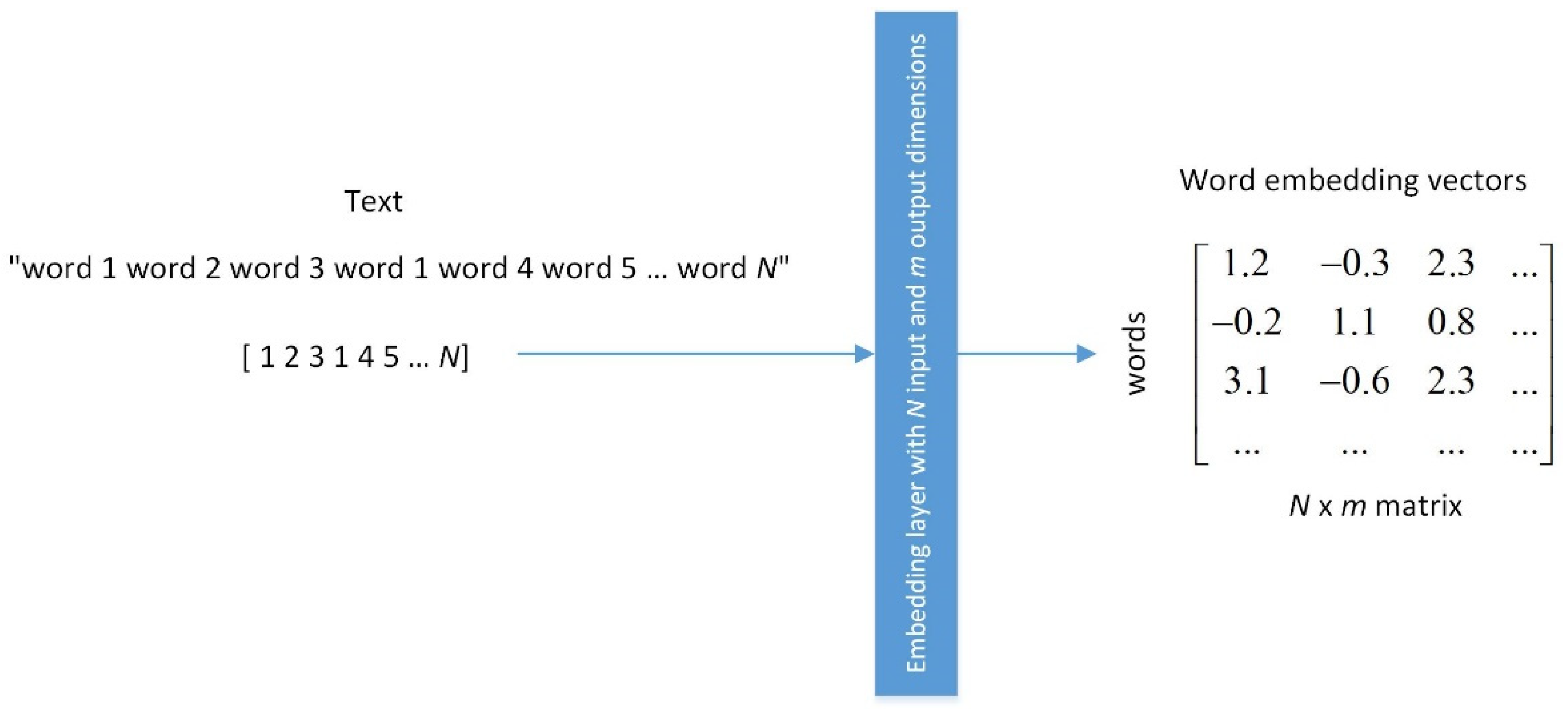
2.1.1. Word Embedding Layer

The embedding layer contains a dense representation of words and their associated semantic relationships. Dense representation is encoding each word with a unique real number [35]. For example, if we have a sentence consists of six words as following “word1 word2 word3 word1 word4 word5”, each word will be encoded with a unique number, and the previous sentence would be represented as the following dense vector of [1 2 3 1 4 5]. The embedding layer encodes each word from the dense representation of N words in a fixed-length embedding vector of length m in real numbers, where N is the number of the words or features as the input of the network and m is the dimension of the embedding (Figure 1).
In this method, related words have close or similar encoding after training [36]. This is accomplished by predicting the context words associated with a given center word within a window of fixed size k. For example, if we have a window of size k = 3 we would have through the text three words inside this window   [ , w j 1 , w j , w j + 1 , ] , where w j 1 and w j + 1 are context words symbolized as w o and w c is a center word symbolized as w c . Following that, a vector representation is assigned to each word w a vector V when the word is a center word w c and a vector U when the word is a context word w o . The length of vectors V and U is equal to the fixed-length embedding   m . By combining these vectors, the word embedding is built. The prediction process is defined by finding the possibility that a context word w o is in the connection of center word w c and calculated as the following [37,38]:
P ( w o | w c ) = exp ( U w o T V w c ) w = 1 N exp ( U w T V w c ) ,
where P ( w o | w c ) is the vector of possibilities that a context word w o is in the connection of center word w c ; U w o T is the transpose of the embedding vector representation of the context word w o ; V w c is the embedding vector representation of the center word w c ; w is the location of the word in the text of N number of words; N is the number of words in the text, and U w T is the transpose of the embedding vector representation of the word in the location w as a context word.
The learning process in words embedding aims at calculating the vectors V and U , as well as building the embedding. To get a high probability using Equation (1), we want to maximize the objective function in a fixed window of the size equal to k along with the whole set of the N size words. The objective function equation is giving as the following [38]:
O = i = 1 N k j k P ( w i + j | w i ) ,
where O is the objective function; N is the number of words in the text; i and j are counters; k is the size of the window, and P ( w i + j | w i ) is the vector of possibilities that a context word w i + j is in the connection of center word w i .
To aid estimation, instead of maximizing Equation (2), we take the average negative logarithm of Equation (2) to derive the loss function and attempt to minimize it. The loss function equation is now given as the following [38]:
L = 1 N i = 1 N k j k log ( P ( w i + j | w i ) )
where L is the loss function; N is the number of words in the text; i and j are counters; k is the size of the window, and P ( w i + j | w i ) is the vector of possibilities that a context word w i + j is in the connection of center word w i .
Using Equations (1) and (3), the model builds the embedding vectors of the words to be ready to send to convolutional and separable convolutional layers in the next steps. Essentially, the embedding layer stores the words embedding, and it is capable of looking up words embedding for a given word and compute gradients in the backward pass. Due to the fixed length of word vectors (words embedding), we can more accurately describe words while still reducing their dimensions. In this way, the embedding layer helps to reduce dimensionality by controlling the number of the features used in training (the features are the input words chosen because of their high frequency of appearing in the training texts). Also, they are able to discover contextual relationships, which means close words; for example, the word “nice” and the word “good” would have close vectors [39]. Words embedding can be discovered and reused by the model across projects using text data. Additionally, it is possible to generate content and language features that can be learned in conjunction with neural network training: they can be learned as a part of the process of adapting a neural network to text [40].

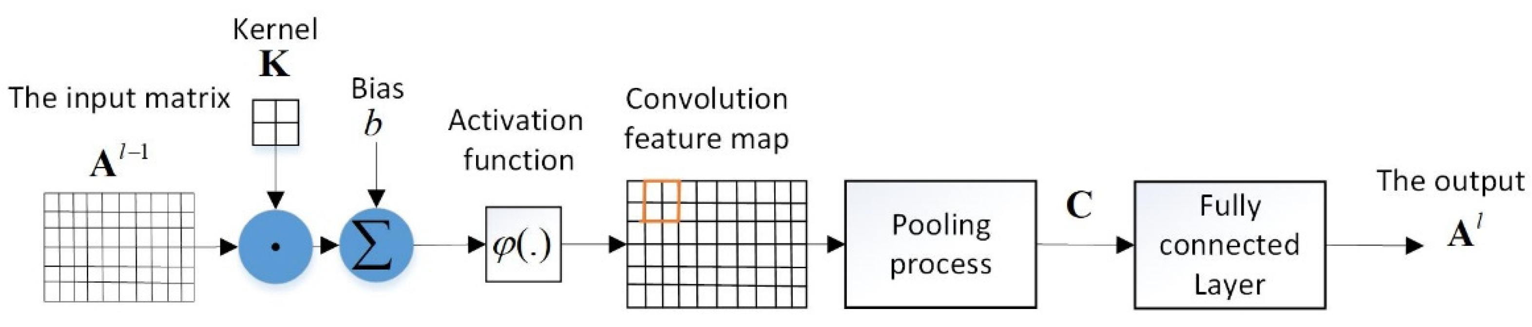
2.1.2. Convolutional, Pooling and Fully Connected Layers

The convolutional layer exhibits high adaptability and is especially adept at mining data with local characteristics. The shared network structure’s weights make it more analogous to the brain’s neural networks, simplifies the network model, and reduces the number of weights. Usually, before performing the convolution product, padding is added around the input matrix to account for the elements on the edges. By convention, padding is done with zeros, and the padding parameter is referred to as p . The padding parameter specifies the number of elements added to each of the input’s four sides. The stride s in the convolution product is the step taken from the filter or the kernel on the input matrix; therefore, a big stride enables the output to be shrunk in size and vice versa. After that, a sampling process is achieved, where the number of elements of each neighborhood go through a pooling process and become one element. Convolution neural layers’ defining technology is the local receptive field, weight sharing, and subsampling by time or space, which extract features and reduce the size of the training parameters, and text feature extraction is critical for text classification because it directly affects the classification’s accuracy [41].
Convolutional, pooling and fully connected layers are shown in Figure 2. The convolutional layer performs a convolution product on two matrices, one of which ( K ) contains the learnable parameters known as a kernel or filter, and the other of which ( A l 1 ) contains the layer’s data or the input layer, ( l 1 ) is devoted to the input layer of the l -th layer. The kernel is a trainable filter K with a size smaller than the input’s size. A convolution feature map results from the following sequential operations: the convolution of the input A l 1 and the kernel K , adding bias b and then passing through an activation function φ (Figure 2). A pooling process is achieved on the convolution feature map to get the matrix C then this matrix is sent to a fully connected layer to give the final output A l [41,42].
To calculate the convolution product between the input matrix A l 1 and the kernel matrix K is used the following equation:
Conv ( A l 1 , K ) = φ ( i = 1 n h j = 1 n w A i , j l 1 K + b ) ,
where Conv ( A l 1 , K ) is the convolution product of the input matrix A l 1 of size ( n h × n w ) with the kernel (filter) matrix K of size ( f × f ) ; A i , j l 1 is a partial matrix of the size of ( f × f ) that is designed in the position ( i , j ) of matrix A l 1 ; b is the bias of the convolution product; φ is the activation function.
The dimension of the resulting product from Equation (4) is given as follows:
Dim ( Conv ( A l 1 , K ) ) = ( n h + 2 p f s + 1 , n w + 2 p f s + 1 ) ,
where Dim ( Conv ( A l 1 , K ) ) is the dimension of the convolution product; p is the padding parameter; and s is the number of strides.
After calculating the output based on Equation (4), we pass it through a pooling process. Parameters are not required to be learned for the pooling process. It is a step in which the matrix features are downsampled by summing the data based on the dimensions determined by Equation (5). The output of the pooling layer is considered to be matrix C (Figure 2). Output C is sent to the fully connected layer shown in Figure 2 to calculate the final output A l . The final output A l is calculated according to equation:
A l = φ ( C W + d ) ,
where C is the output matrix of the pooling layer; W , d , φ are the matrix of weights, the bias and the activation function of the fully connected layer, respectively.

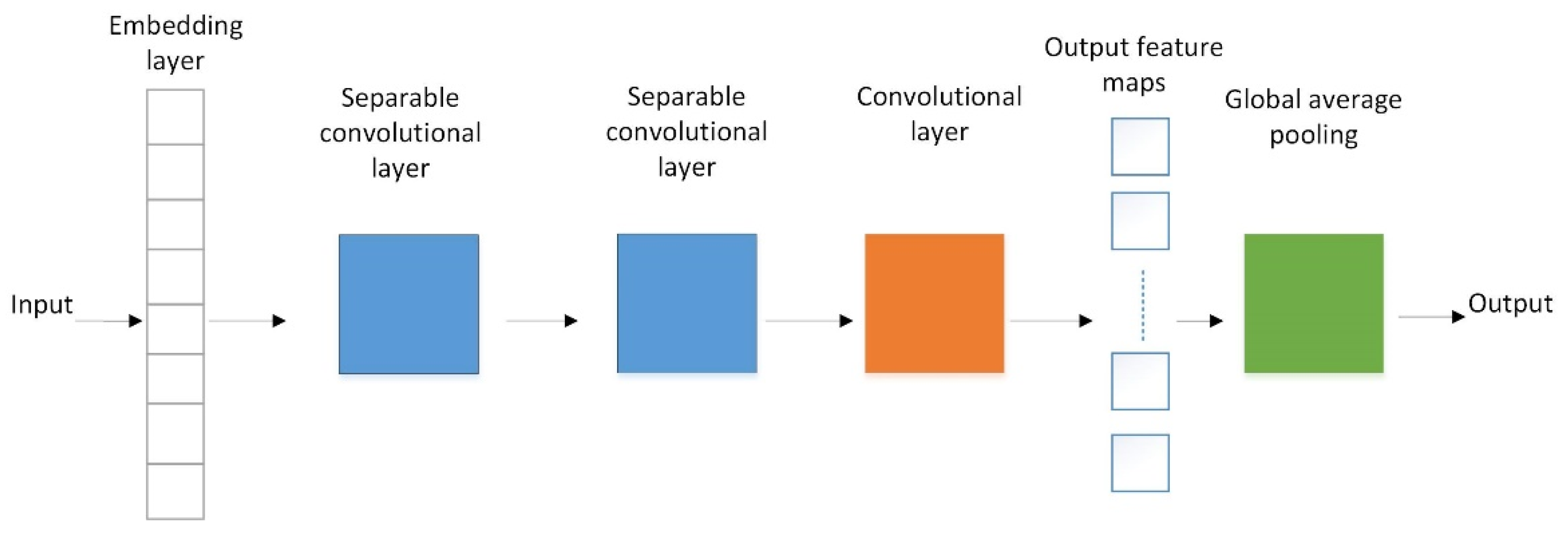
2.2. Separable Convolutional Neural Network with Embedding Layer and Global Average Pooling

The text classification model in our work uses the network layers, which are depicted in Figure 3. We see the embedding layer like in Figure 2 that is described in Section 2.1, three deep layers (two separable and one normal convolutional layers), as well as a global average pooling that replaces two blocks (“Pooling process” and “Fully connected layer”) in Figure 2. We call the network with structure the separable convolutional neural network in Figure 3.
Two deep neural layers for the main feature extraction of the input are separable convolutional layers instead of one normal convolutional layer. The aim of these deep layers is to reduce the model complexity and to decrease the required amount of training. The third deep layer is a convolutional layer with several neurons corresponding to the output categories. The third convolutional layer produces an output on the shape of feature maps. Therefore, to transfer each feature map to a single output, a global average pooling layer in Figure 3 is used to achieve the goal of classification without adding extra trainable parameters to the model. Furthermore, we describe separable layer and global average pooling.
The following is a comparison of the proposed SCNN structure with the structure represented in [31] and emphasizes their differences. The SCNN structure in [31] composes the unit named “Multiple separable convolutional blocks,” which means a depthwise separable convolution [29,30]. This convolution is fulfilled independently over each channel of an input signal. The parting into some channels is applied, as a rule, in the case of image processing, which is why we did not include this unit in our structure. However, for generality, this unit can be placed in the structure shown in Figure 3. Separable convolutional layers, which are used in Figure 3 and in [31], execute a pointwise separable convolution [32,33] and make a neural network simpler. However, sometimes this approach does not provide enough accuracy. We included a convolutional layer in addition to separable convolutional layers in order to increase the classification accuracy. This way is more preferable in comparison with the use of multiple fully connected layers, which are placed behind the unit “Global average pooling and dropout” [31] and serve to increase accuracy. The number of parameters in a convolutional layer is known to be much less than in a multiple fully connected layer.

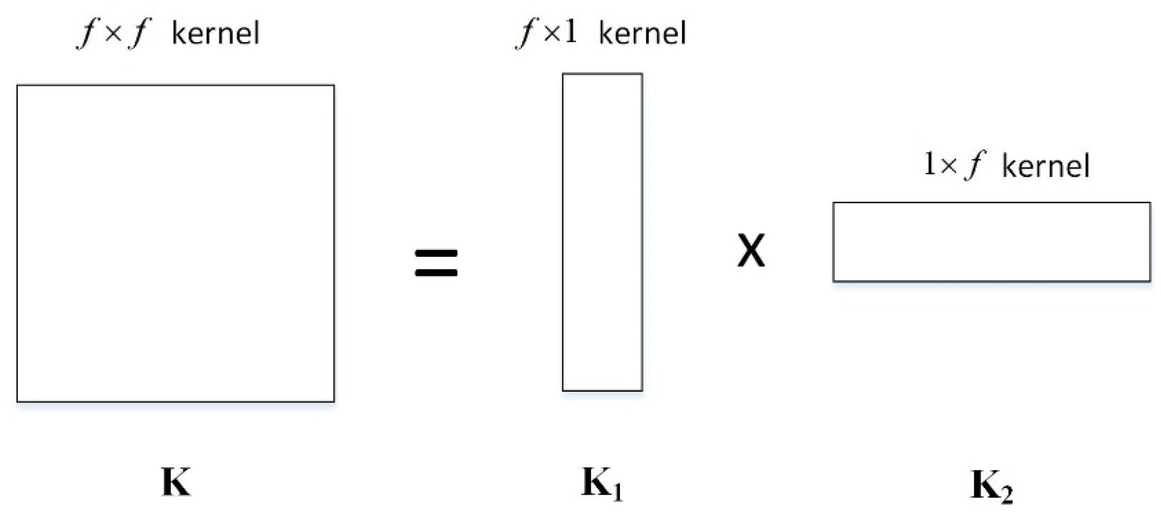
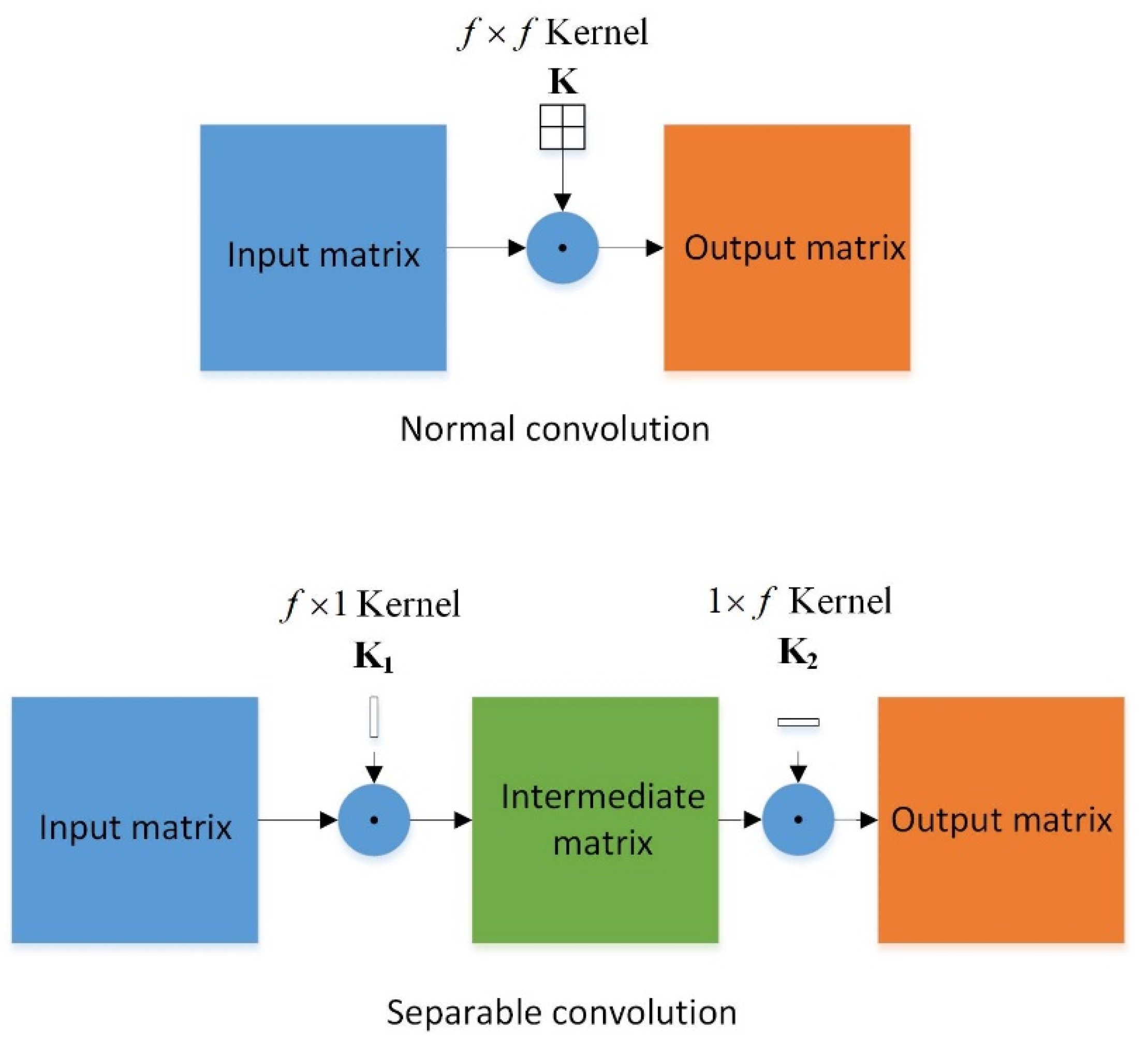
2.2.1. Separable Convolutional Layer

Separable convolutional layers are exclusively associated with dimensions related to the spatial dimensions and are also known as the separable spatial convolution, as it is focused on one of the widths and one of the heights. They were developed because an issue arises when deep neural networks have many convolutional layers; this is especially true for multilayer networks. For these procedures, a significant amount of training is required [43]. Spatial separable convolution calculates a filter by recursively breaking a kernel into two pieces. For example, the ( f × f ) size of kernel K can be done with ( f × 1 ) of kernel K 1 and ( 1 × f ) of kernel K 2 (Figure 4), where K = K 1 × K 2 .
Thus, instead of doing one iteration of nine multiplications, we do two convolutions, which have the same effect. In other words, rather than doing a two-dimensional convolution with K , the same result is attended by doing two one-dimensional convolutions with K 1 and K 2 . Therefore, computational complexity goes down, and the network is able to run faster. This process will have two steps, as shown in Figure 5.
The number of multiplications is reduced, and so computational complexity is also reduced, allowing the network to run faster [44]. Spatially separable convolutions relieve the need for material resources to training standard convolutional networks. To describe the separable convolution product, we have two equations:
A ¯ l 1 = Conv ( A l 1 , K 1 ) = i = 1 n h j = 1 n w A i , j l 1 K 1 ,
Conv ( A ¯ l 1 , K 2 ) = i = 1 ( n h + 2 p f ) / s + 1 j = 1 n w K 2 A ¯ i , j l 1 ,
where A ¯ l 1 is the convolution product of the input matrix A l 1 with the kernel or filter K 1 , it is a matrix of size ( ( ( n h + 2 p f ) / s + 1 ) × n w ) ; p is the padding parameter; s is the number of strides; K 1 is the kernel vector of size ( f × 1 ) ; A l 1 is the input matrix of size ( n h × n w ) ; A i , j l 1 is a partial column vector of size ( f × 1 ) , that is designed in the position ( i , j ) of matrix A l - 1 ; K 2 is the kernel vector of size ( 1 × f ) ; A ¯ i , j l 1 is a partial row vector of size ( 1 × f ) , that is designed in the position ( i , j ) of matrix A ¯ l 1 . The convolution products of Equations (7) and (8) replace the convolution product in Equation (4), and the process follows the same calculation of Equations (5) and (6).
Due to their ability to separate convolutional layers along their spatial axis, they enable the splitting of large convolutional layers into smaller ones that produce the same result when convolved sequentially. As a result, the number of times that must be multiplied to obtain the same result decreases [45,46]. Separable convolutions begin with a depth wise-spatial convolution (which acts separately on each input channel) and end with a pointwise convolution that mixes the resulting output channels, and separable convolutional neural networks can fully exploit the inherent characteristics of the data, such as localization, optimize the network structure, and maintain a degree of displacement invariance.

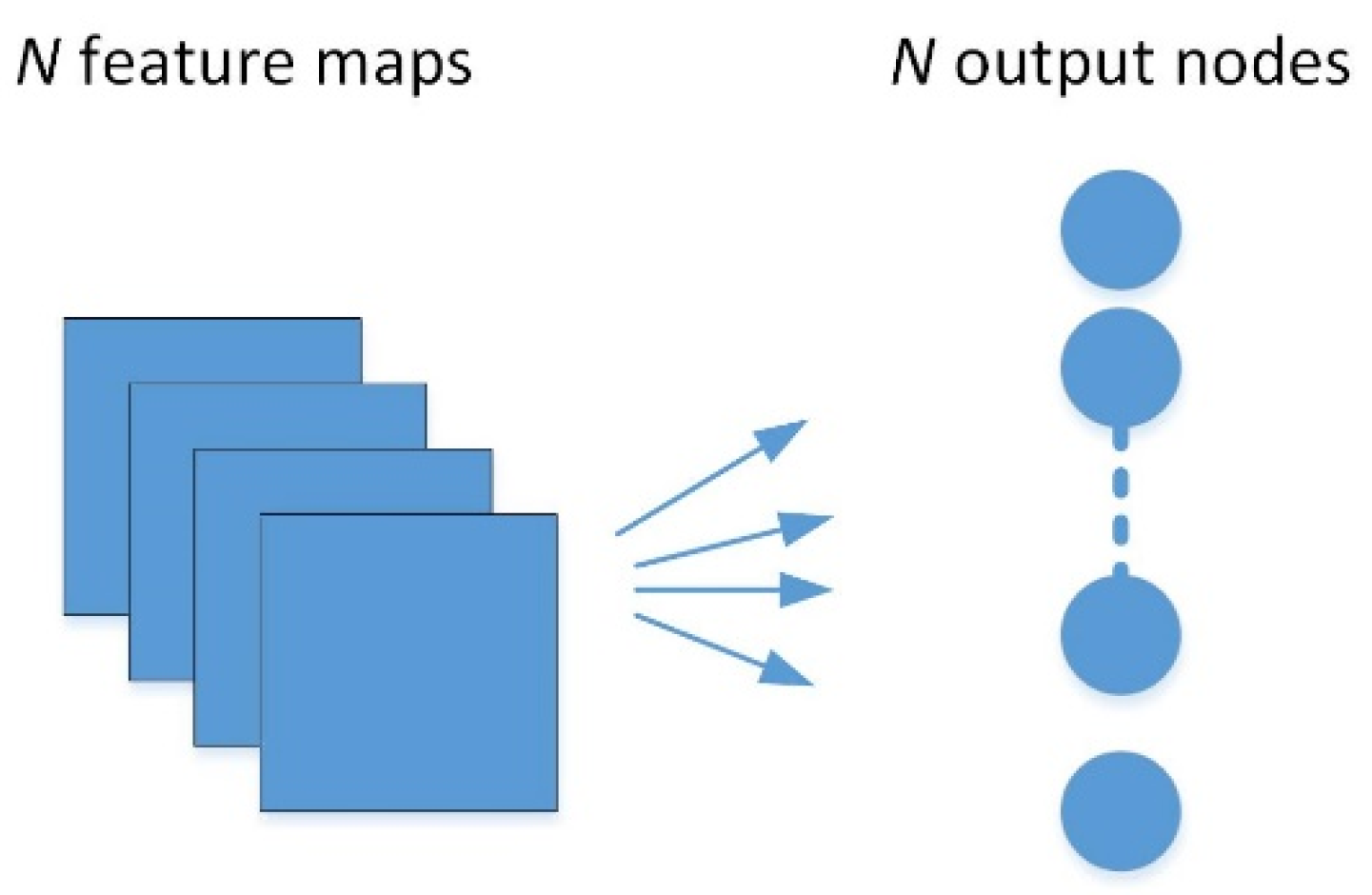
2.2.2. Global Average Pooling

Global average pooling can be used instead of “Pooling process” and “Fully connected layer” in Figure 2, and it determines the average output of each feature map in the preceding layer. The aim of the final convolutional layer is to produce a feature map for each category in the classification task. The pool size is equal to the size of the output of the last convolutional layer (Figure 6). Instead of stacking layers on top of fully connected networks, the Softmax function is applied on all of the feature maps and inserts them in the output, resulting in a vector [47,48].
In contrast to the fully connected layer, which could cause some issues with the feature maps not being highly local, global average pooling has better performance since it imposes a direct correspondence between feature map/categorical representation [49]. In addition, it can be concluded that function maps can easily be interpreted as trusted maps for categories. To this extent, since there is no ability to fine-tune the global averaging, this pooling layer has no problem with overfitting. Additionally, since global average pooling aggregates spatial information, it is more resilient to input spatial translations [50].

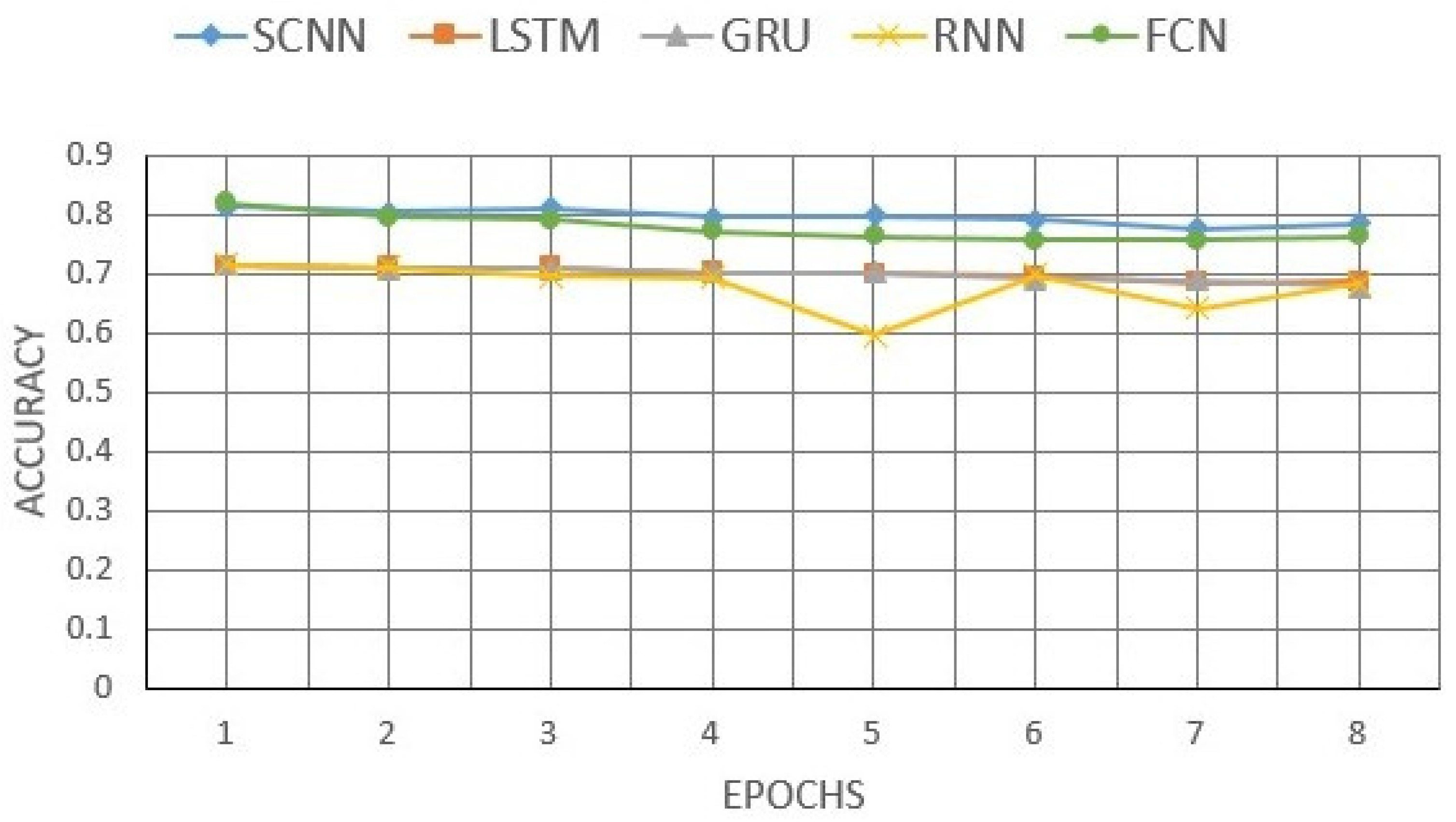
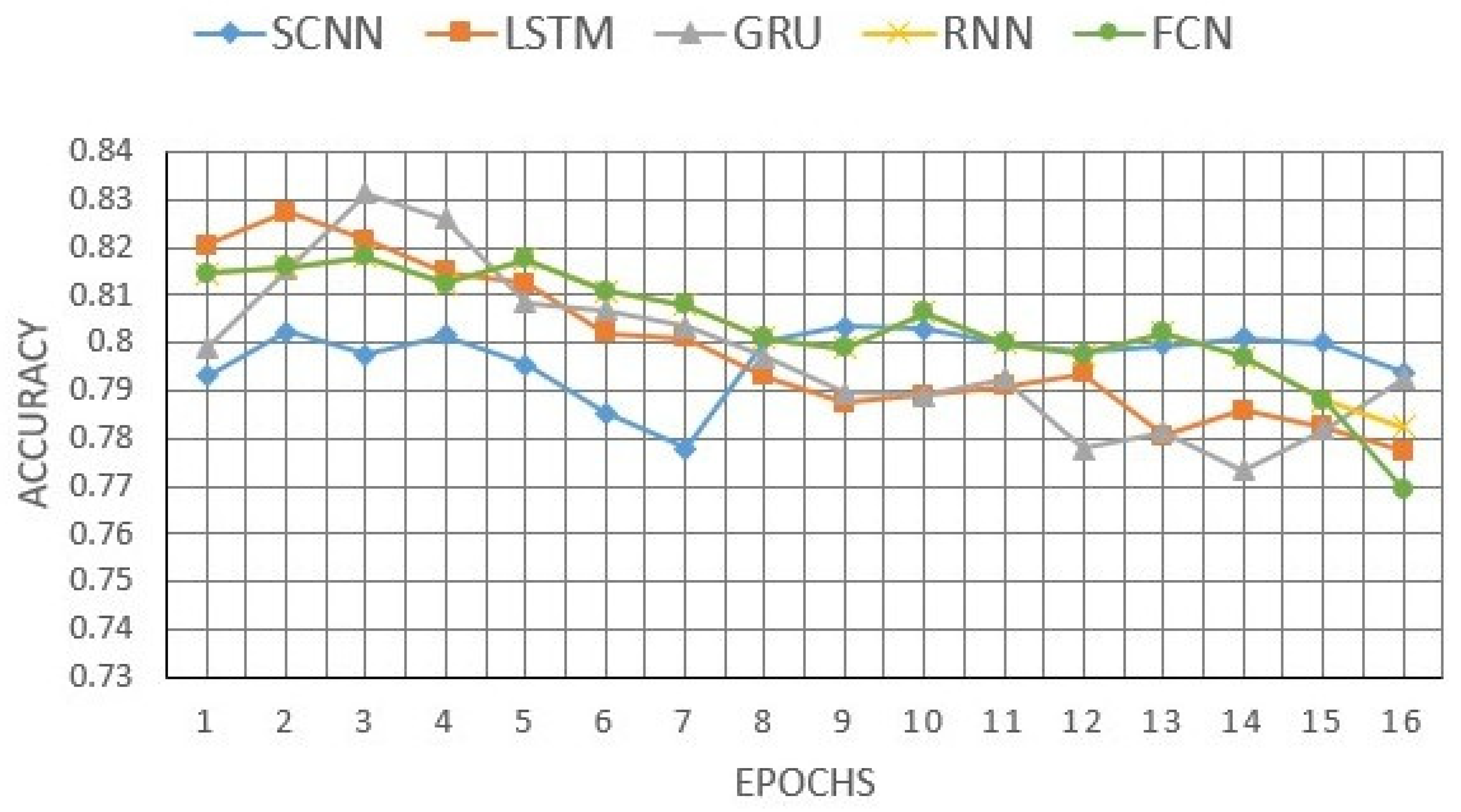
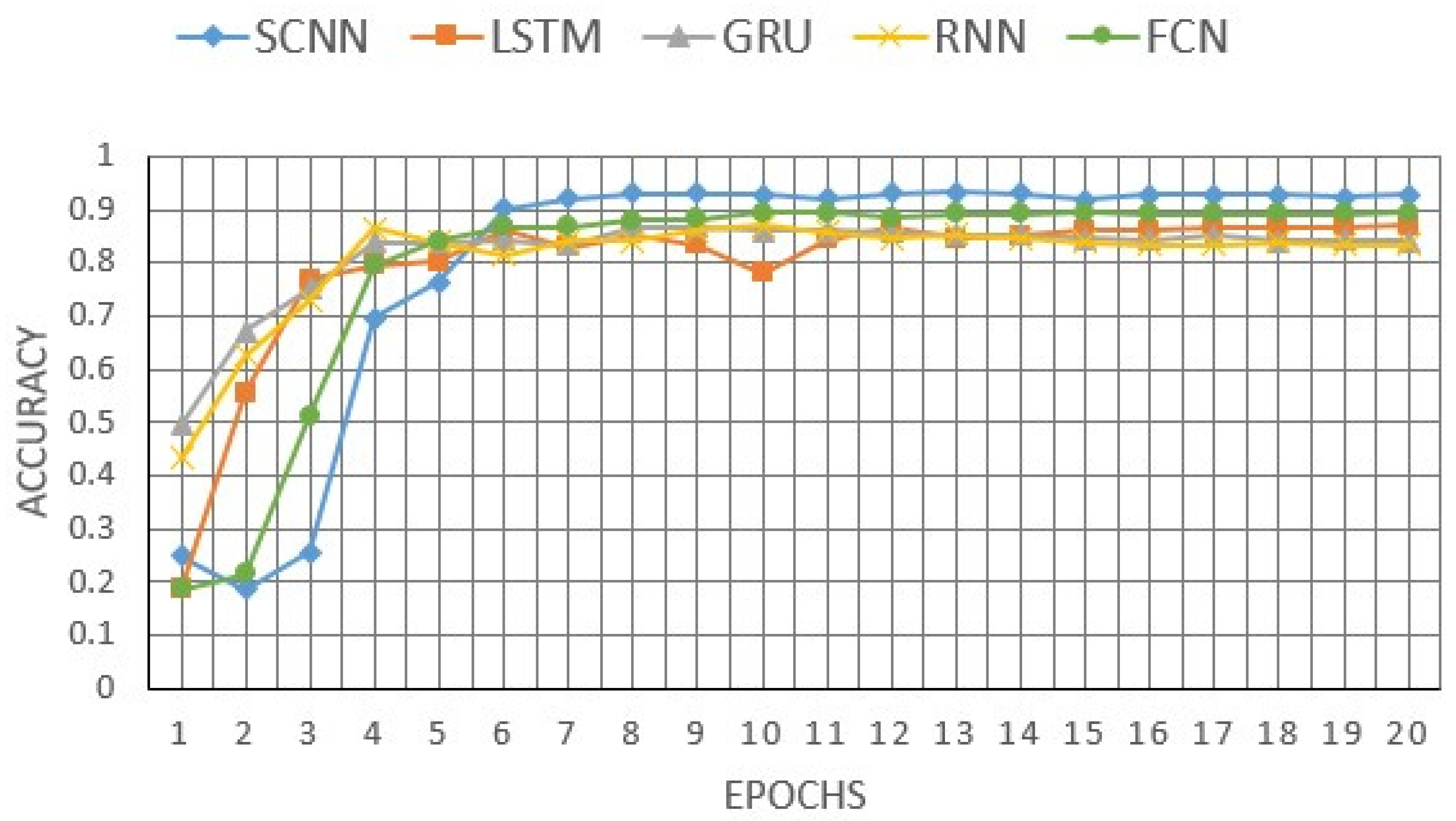
3. Results of Binary and Multiclass Text Classifications

In our practical experiment, we used Python 3.7.9 and TensorFlow 2.3.0 with a Pycharm.3.1 2019 environment on Asus X556U Core i7 7500U 3.5 Hz.
We start with the binary classification using the IMDB database from the TensorFlow library database for training our neural networks and the IMDB database from the NLTK corpus library database for testing our neural networks. The binary classification criteria are based on two sets of movie reviews, the first set is positive reviews of movies, and the second is negative movie reviews. The multiclass classification criteria are based on five sets of articles in the fields of business, entertainment, politics, sport, and technology. For binary sentiment classification, the IMDB database extracted from TensorFlow’s database is a substantial movie review dataset with significantly more data than other available benchmark datasets. It includes a training set of 25,000 movie reviews, a testing set of 25,000 movie reviews, and more unlabeled data for use. However, we used both the training set and testing set as a large training set of 50,000 reviews for training our neural networks. On the other hand, our testing data consist of 2000 files from the IMDB of the NLTK corpus library. For the multiclass classification problem, the BBC database was used. With regards to this database, there are very dense collections of text documents that business organizations can use as a large source of data. This collection of articles contains a total of 2225 articles organized into five broad categories: business, entertainment, politics, sport, and technology. Each category contains 445 big articles; these articles were divided into 1557 ones for training and 668 ones for testing.
In our study, we compared the performance of our suggested model of separable convolutional neural networks and convolutional neural networks with four other types of neural networks: Recurrent Neural Network (RNN), Long Short-Term Memory (LSTM), Gated Recurrent Unit (GRU), and Fully Connected Network (FCN). Both the LSTM and the GRU are recurrent neural networks where each recurrent layer contains feedback loops. This enables them to retain data in memory over time. Nevertheless, training standard the RNNs to resolve difficulties needing the acquisition of long-term temporal dependencies can be difficult. As the loss function’s gradient decays exponentially with time, the loss function should lose precision rapidly. The LSTM is a type of recurrent neural network that applies non-standard units in addition to standard ones. The LSTM units incorporate a memory cell capable of storing data for an outspread duration. A series of gates are used to control the flow of information into and out of the memory and when it is forgotten. This architecture enables them to develop longer-term reliance. GRUs, like LSTMs, employ a set of gates to regulate information flow, but they do so without using separate memory cells and with fewer gates.
The LSTM addresses the issues of gradient vanishing in the standard RNN by including new gates, such as input gate and forget gate, which improves the gradient flow and preserves long-range dependencies. The long-range dependence existing in the RNN is solved in the LSTM by means of the addition of the repeating layers. The critical distinction between the GRU and the LSTM is that the GRU holds two gates: reset gate and update gate, whereas the LSTM has three gates: input, output, and forget. The GRU is less complicated than the LSTM because it uses only two gates, therefore fewer training parameters. As a result, it consumes less memory, executes faster, and trains faster than the LSTM, whereas the LSTM is more accurate on datasets with longer sequences. In short, if the sequence is lengthy or precision is critical.
We used two types of activation functions in the last layer; for sigmoid, see Equation (9), and for Softmax, see Equation (10) for the binary classification. The sigmoid function is calculated from equation:
S ( x ) = 1 1 + e x
where S ( x ) is the output of the sigmoid function; x is a scalar argument of the sigmoid function. The Softmax function is calculated from the equation:
Y = exp ( X ) j = 1 K exp ( x j ) ,
where Y = [ y 1 , y 2 , , y K ] , X = [ x 1 , x 2 , , x K ] are the output and input vectors of the Softmax function, respectively; k is the number of the multiclass classes of the classification; j is a counter.
While in the multiclass classifications, we used the Softmax activation function. The sigmoid activation function has a value in the range of 0 to 1, and it is implemented individually to each component of the output. On the other hand, in the Softmax activation function, each element has a value between 0 and 1, but all elements sum to 1. This can be understood as a probability distribution. When given a vector of real numbers, Softmax normalizes it to a probability distribution proportional to the exponential of the input values. Before its application, some of the input values may be negative or larger than 1. As a result, the greater the input number, the greater the probabilities. In conclusion, the main difference between the Softmax and the sigmoid activation function is that we add all of the values in the denominator in Softmax. When computing the value of Softmax on a single vector output, it is not applied independently to each output element but rather to all of the output data, as Softmax activation distributes the probability evenly across each output node.
To study the efficiency of our SCNN, we compare it in the accuracy and the total training and testing time with the FCN, the RNN, the LSTM and the GRU. The models that we build for the comparison have the same number of neurons and the same number of layers as the suggested model. All the described networks have the same first layer. The first layer is the words embedding layer, which contains a dense representation of words and their associated semantic relationships. It has an input of 5000 and an embedding size of 16. In the following is the description of all the above-mentioned networks. This description starts from the second layer.
The FCN used in our comparison consists of five layers. The second layer is a global average pooling layer to reshape the output of the embedding and send this output to the next layer. The third and fourth layers are fully connected layers with 32 and 64 neurons, respectively, and the Relu activation function. For the binary classification, the fifth (the last) layer consists of, in the first case, one neuron with the sigmoid function and, in the second case, two neurons with the Softmax functions. For the multiclass classifications, the fifth layer contains six neurons with the Softmax functions.
The RNN, the LSTM, and the GRU consist of five layers. The embedding layer is followed by two layers with 32 and 64 neurons, respectively, and the tangent activation function. After the two layers are designed according to the RNN, LSTM and GRU structures [51], there is the fourth layer, which is a global average pooling layer, to reshape the output and send it to the fifth layer. The fifth layer is a fully connected network. For the binary classification, the fifth (the last) layer consists of, in the first case, one neuron with the sigmoid function and, in the second case, two neurons with the Softmax functions. For the multiclass classifications, the fifth layer contains six neurons with the Softmax functions.
The SCNN consists of five layers as we can see in Figure 3. The first layer is the embedding layer. The second layer is a separable convolutional layer with 32 neurons; every neuron is described by two separated kernels of the 2 × 1 and the 1 × 2 sizes and the Relu activation function. The third layer is a separable convolutional layer with 64 neurons; every neuron is described by two separable kernels of the 8 × 1 and the 1 × 8 sizes and the Relu activation function. The fourth layer is a convolutional layer, including one neuron with the sigmoid function for the first binary classification, two neurons with the Softmax function for the second binary classification, and six neurons with the Softmax function for the multiclass classification. Every neuron of the convolutional layer is described by the kernel of the 3 × 3 size. The fifth (the last) layer is a global average pooling layer to reshape the output of the convolutional layer.
To compare the above-mentioned neural networks, we calculate the number of the network parameters, the sum of training and testing time and the accuracy of the written test texts’ classification. The accuracy D is defined in the testing stage as follows:
D = N c N t × 100 % ,
where N c is the number of the correct (true) predictions and N t is the number of the total elements of the testing set.
The training and testing process of each model consists of epochs. An epoch is a terminology used in machine learning that refers to the number of times the machine learning model has crossed the whole training dataset and after that performed testing on the whole testing dataset. In each epoch, the weights of the neural network of the models get updated using the training set. Then at the end of each epoch, the model performs a prediction process or a testing process on the testing dataset using Equation (11) to calculate the accuracy of the performance at each epoch. Nevertheless, the testing set is not included in the training set, and it is completely unknown for the model.
The development of accuracy is illustrated in Figure 7 for the binary classification with sigmoid activation function, Figure 8 for the binary classification with the Softmax activation function, and Figure 9 for the multiclass classification. The parameters of training and the final testing accuracies are shown in Table 1 for the binary classification with sigmoid activation function, Table 2 for the binary classification with the Softmax activation function, and Table 3 for the multiclass classification.
In our experiment, we fulfilled three training processes. In the binary classification under the sigmoid activation function of neural networks, the training and testing processes last eight epochs (Figure 7). As can be seen from Table 1, the proposed SCNN reached the highest accuracy with 78.6% in 150 s, while the other networks achieved a lower accuracy and more calculation time. Thus, the RNN, the GRU, and the LSTM have a close accuracy of around 68%, with a calculation time above 560 s for the GRU and the LSTM and about 240 s for the RNN. In this part of the study, the FCN reached a better accuracy with 76.4% and the lowest calculation time, around 25 s in comparison with the three different types of recurrent neural networks.
In the binary classification with Softmax function, the training process lasts 16 epochs (Figure 8). We can see from Table 2 that the proposed SCNN model reached the highest accuracy with 79.4% in 312 s. The other networks achieved a lower accuracy in the same number of epochs and more calculation time. The RNN, the GRU, and the LSTM have a close accuracy of around 78%, with a training time above 1850 s. The FCN reached the lowest accuracy with 76.95% and the lowest time of calculation (around 43 s) in comparison to the mentioned recurrent neural networks. We notice that using the Softmax activation function to deal with the binary classification as multiclass classifications with two classes improves the accuracy in all the represented neural networks.
In the multiclass classification, the calculation process lasts 20 epochs. We can see from Table 3 that the proposed SCNN reached the highest accuracy with 92.81% in 13 s, while the other networks achieved a lower accuracy and more calculation time. The FCN achieved 89.5% in 4 s of calculation. The LTSM achieved 87% in 126 s. The GRU and the RNN achieved a close accuracy of 84% in 117 s for the GRU and 65 s for the RNN.
As follows from the analysis of Table 1, Table 2 and Table 3, the design of the SCNN provides the quality to be more specialized and efficient than the other represented neural networks. In the SCNN, the number of parameters is reduced and the learning process is accelerated.

4. Conclusions

Texts constantly tell and express something of importance. Written language showed that we could find sufficient information from texts. In order to achieve different analyses over a vast number of texts, we have to solve the fundamental problem, which is categorizing texts and classifying them. In natural language processing, we achieved three classifications of written texts: a binary classification with the sigmoid activation function in the last layer of the neural network, a binary classification with the Softmax activation function in the last layer, and multiclass classifications with the Softmax activation function. We proposed combining the convolutional and separable convolutional layers to solve the classification problem and compare the SCNN with the other neural network such as the RNN, the GRU, the LSTM, and the FCN.
The results of the investigation show that using the SCNN for binary and multiclass classifications gives
  • Higher accuracy reached 79.4% in the case of the Softmax activation function in the last layer of the network (this accuracy exceeds 78.6% in the case of the sigmoid activation function), and 92.81% for the multiclass classification.
  • Lower computation complexity. Using the separable convolutional layer reduced the learning parameters of the network with keeping its ability of feature extraction enabling the data to be expressed as spatial with the locally and equally possible to occur extracted features at any input.
  • Fast calculation time. The lower computation complexity reduced the training and testing time of the SCNN without affecting its quality and accuracy.
The study’s results show how the combination of separable and normal convolutional layers in deep learning with the field of natural language processing and data mining expands the possibilities for achieving better quality demonstrated with the high accuracy, low complexity, and fast calculation. At the same time, the SCNN has a connection pattern formed as a grid of neurons where each neuron is connected with all the surrounding neurons. The connectivity pattern between neurons inspires this connection pattern that matches the organization of the human brain cortex. This increases its accuracy in comparison with the other neural networks because this pattern provides the ability of feature extraction allowing the data to be expressed as spatial with the locally and equally possible to occur extracted features at any input.
The RNN, the LSTM, and the GRU have a recurrent methodology which makes the computational process slower. Using tanh as activation functions makes the training difficult to process very long sequences. The LSTM is inclined to overfitting, even more so when the input and recurrent connections to long short-term memory units are eliminated from activation and weight updates during network training. The GRU shares many of the downsides of the RNN and the LSTM; it also has a slow convergence rate and a low learning efficiency. The FCN lacks the ability of feature extraction of the CNN and the ability to process long related inputs like the RNN, the GRU, and the LSTM. Eventually, due to the architecture of the FCN, each node is connected to another via a dense web, resulting in redundancy and inefficiency.

Author Contributions

Conceptualization, E.S. and A.A.; methodology, E.S. and A.A.; software, A.A.; validation, E.S. and A.A.; formal analysis, E.S. and A.A.; investigation, E.S. and A.A.; resources, E.S.; data curation, A.A.; writing—original draft preparation, E.S. and A.A.; writing—review and editing, E.S. and A.A.; visualization, A.A.; supervision, E.S.; project administration, E.S.; funding acquisition, E.S. All authors have read and agreed to the published version of the manuscript.

Funding

This research received no external funding.

Institutional Review Board Statement

Not applicable.

Informed Consent Statement

Not applicable.

Data Availability Statement

Not applicable.

Conflicts of Interest

The authors declare no conflict of interest.

References

  1. Ghavami, P. Big Data Analytic Methods, 2nd ed.; Walter de Gruyter Inc.: Berlin, Germany, 2020; pp. 65–88. [Google Scholar] [CrossRef]
  2. Hong, T.; Choi, J.A.; Lim, K.; Kim, P. Enhancing Personalized Ads Using Interest Category Classification of SNS Users Based on Deep Neural Networks. Sensors 2020, 21, 199. [Google Scholar] [CrossRef]
  3. Collins, E.; Rozanov, N.; Zhang, B. Evolutionary Data Measures: Understanding the Difficulty of Text Classification Tasks. In Proceedings of the 22nd Conference on Computational Natural Language Learning, Brussels, Belgium, 31 October–1 November 2018; pp. 380–391. [Google Scholar] [CrossRef]
  4. Han, S. Predictive Analytics: Semi-Supervised Learning Classification Based on Generalized Additive Logistic Regression for Corporate Credit Anomaly Detection. IEEE Access 2020, 8, 199060–199069. [Google Scholar] [CrossRef]
  5. Lee, W.M. Python® Machine Learning, 1st ed.; John Wiley & Sons Inc.: Indianapolis, IN, USA, 2019; pp. 151–175. [Google Scholar] [CrossRef]
  6. Tamhane, A.C. Predictive Analytics: Parametric Models for Regression and Classification Using R, 1st ed.; John Wiley & Sons Inc.: Hoboken, NJ, USA, 2021; pp. 181–224. [Google Scholar] [CrossRef]
  7. Tan, Y.; Shenoy, P.P. A bias-variance based heuristic for constructing a hybrid logistic regression-naïve Bayes model for classification. Int. J. Approx. Reason. 2020, 117, 15–28. [Google Scholar] [CrossRef]
  8. Kim, H.; Kim, J.; Kim, J.; Lim, P. Towards perfect text classification with Wikipedia-based semantic Naïve Bayes learning. Neurocomputing 2018, 315, 128–134. [Google Scholar] [CrossRef]
  9. Islamiyah; Dengen, N.; Maria, E. Naïve Bayes Classifiers for Tweet Sentiment Analysis Using GPU. Int. J. Eng. Adv. Technol. 2019, 8, 1470–1472. [Google Scholar] [CrossRef]
  10. Xi, X.; Zhang, F.; Li, X. Dual Random Projection for Linear Support Vector Machine. DEStech Trans. Comput. Sci. Eng. 2017, 173–180. [Google Scholar] [CrossRef] [Green Version]
  11. Singh, C.; Walia, E.; Kaur, K.P. Enhancing color image retrieval performance with feature fusion and non-linear support vector machine classifier. Optik 2018, 158, 127–141. [Google Scholar] [CrossRef]
  12. Sirignano, J.; Spiliopoulos, K. Stochastic Gradient Descent in Continuous Time: A Central Limit Theorem. Stoch. Syst. 2020, 10, 124–151. [Google Scholar] [CrossRef]
  13. Kowsari, K.; Brown, D.E.; Heidarysafa, M.; Meimandi, K.J.; Gerber, M.S.; Barnes, L.E. Hdltex: Hierarchical deep learning for text classification. In Proceedings of the 16th IEEE International Conference on Machine Learning and Applications (ICMLA), Cancun, Mexico, 18–21 December 2017; pp. 364–371. [Google Scholar] [CrossRef] [Green Version]
  14. Prusa, J.D.; Khoshgoftaar, T.M. Designing a Better Data Representation for Deep Neural Networks and Text Classification. In Proceedings of the 2016 IEEE 17th International Conference on Information Reuse and Integration (IRI), Pittsburgh, PA, USA, 28–30 July 2016; pp. 411–416. [Google Scholar] [CrossRef]
  15. Amato, F.; Mazzocca, N.; Moscato, F.; Vivenzio, E. Multilayer Perceptron: An Intelligent Model for Classification and Intrusion Detection. In Proceedings of the 31st International Conference on Advanced Information Networking and Applications Workshops (WAINA), Taipei, Taiwan, 27–29 March 2017; pp. 686–691. [Google Scholar] [CrossRef]
  16. Prastowo, E.Y.; Endroyono; Yuniarno, E. Combining SentiStrength and Multilayer Perceptron in Twitter Sentiment Classification. In Proceedings of the 2019 International Seminar on Intelligent Technology and Its Applications (ISITIA), Surabaya, Indonesia, 28–29 August 2019; pp. 381–386. [Google Scholar] [CrossRef]
  17. Solovyeva, E.B.; Degtyarev, S.A. Synthesis of Neural Pulse Interference Filters for Image Restoration. Radioelectron. Commun. Syst. 2008, 51, 661–668. [Google Scholar] [CrossRef]
  18. Solovyeva, E.B.; Inshakov, Y.M.; Ezerov, K.S. Using the NI ELVIS II Complex for Improvement of Laboratory Course in Electrical Engineering. In Proceedings of the 2018 IEEE International Conference “Quality Management, Transport and Information Security, Information Technologies” (IT&MQ&IS), St. Petersburg, Russia, 24−28 September 2018; pp. 725–730. [Google Scholar] [CrossRef]
  19. Solovyeva, E. A Split Signal Polynomial as a Model of an Impulse Noise Filter for Speech Signal Recovery. J. Phys. Conf. Ser. (JPCS) 2017, 803, 012156. [Google Scholar] [CrossRef]
  20. Zhao, Y.; Shen, Y.; Yao, J. Recurrent Neural Network for Text Classification with Hierarchical Multiscale Dense Connections. In Proceedings of the Twenty-Eighth International Joint Conference on Artificial Intelligence, Macao, China, 10–16 August 2019; pp. 5450–5456. [Google Scholar] [CrossRef] [Green Version]
  21. Buber, E.; Diri, B. Web Page Classification Using RNN. Procedia Comput. Sci. 2019, 154, 62–72. [Google Scholar] [CrossRef]
  22. Son, G.; Kwon, S.; Park, N. Gender Classification Based on The Non-Lexical Cues of Emergency Calls with Recurrent Neural Networks (RNN). Symmetry 2019, 11, 525. [Google Scholar] [CrossRef] [Green Version]
  23. Solovyeva, E. Types of Recurrent Neural Networks for Non-linear Dynamic System Modelling. In Proceedings of the 2017 IEEE International Conference on Soft Computing and Measurements (SCM2017), St. Petersburg, Russia, 24−26 May 2017; pp. 252–255. [Google Scholar] [CrossRef]
  24. Song, P.; Geng, C.; Li, Z. Research on Text Classification Based on Convolutional Neural Network. In Proceedings of the International Conference on Computer Network, Electronic and Automation (ICCNEA), Xi’an, China, 27–29 September 2019; pp. 229–232. [Google Scholar] [CrossRef]
  25. Abdulnabi, N.Z.T.; Altun, O. Batch size for training convolutional neural networks for sentence classification. J. Adv. Technol. Eng. Res. 2016, 2, 156–163. [Google Scholar] [CrossRef]
  26. Truşcǎ, M.; Spanakis, G. Hybrid Tiled Convolutional Neural Networks (HTCNN) Text Sentiment Classification. In Proceedings of the 12th International Conference on Agents and Artificial Intelligence, Valletta, Malta, 22–24 February 2020; pp. 506–513. [Google Scholar] [CrossRef]
  27. Tiryaki, O.; Okan Sakar, C. Nonlinear Feature Extraction using Multilayer Perceptron based Alternating Regression for Classification and Multiple-output Regression Problems. In Proceedings of the 7th International Conference on Data Science, Technology and Applications, Porto, Portugal, 26–28 July 2018; pp. 107–117. [Google Scholar] [CrossRef]
  28. Zhang, J.; Li, Y.; Tian, J.; Li, T. LSTM-CNN Hybrid Model for Text Classification. In Proceedings of the IEEE 3rd Advanced Information Technology, Electronic and Automation Control Conference (IAEAC), Chongqing, China, 12–14 October 2018; pp. 1675–1680. [Google Scholar] [CrossRef]
  29. Chollet, F. Xception: Deep Learning with Depthwise Separable Convolutions. In Proceedings of the 2017 IEEE Conference on Computer Vision and Pattern Recognition (CVPR), Honolulu, HI, USA, 21–26 July 2017; pp. 1800–1807. [Google Scholar] [CrossRef] [Green Version]
  30. Kaiser, L.; Gomez, A.N.; Chollet, F. Depthwise Separable Convolutions for Neural Machine Translation. In Proceedings of the ICLR 2018 Conference, Vancouver, BC, Canada, 30 April–3 May 2018; pp. 1–10. [Google Scholar]
  31. Timo, I. Denk. Text Classification with Separable Convolutional Neural Networks, Technical Report for Internship; Baden-Wurttemberg Cooperative State University Karlsruhe: Karlsruhe, Germany, 17 September 2018. [Google Scholar] [CrossRef]
  32. Wang, Y.; Feng, B.; Ding, Y. DSXplore: Optimizing Convolutional Neural Networks via Sliding-Channel Convolutions. In Proceedings of the 2021 IEEE International Parallel and Distributed Processing Symposium (IPDPS), Portland, ON, USA, 17–21 May 2021; pp. 619–628. [Google Scholar] [CrossRef]
  33. Yadav, R. Light-Weighted CNN for Text Classification; Project Report; Technical University of Kaiserslautern: Kaiserslautern, Germany, 16 April 2020. [Google Scholar]
  34. Khanal, J.; Tayara, H.; Chong, K.T. Identifying Enhancers and Their Strength by the Integration of Word Embedding and Convolution Neural Network. IEEE Access 2020, 8, 58369–58376. [Google Scholar] [CrossRef]
  35. Abdulmumin, I.; Galadanci, B.S. hauWE: Hausa Words Embedding for Natural Language Processing. In Proceedings of the 2019 2nd International Conference of the IEEE Nigeria Computer Chapter (Nigeria ComputConf), Zaria, Nigeria, 14–17 October 2019; pp. 1–6. [Google Scholar] [CrossRef] [Green Version]
  36. Pierina, G.A. Bag of Embedding Words for Sentiment Analysis of Tweets. J. Comput. 2019, 14, 223–231. [Google Scholar] [CrossRef]
  37. Xiao, L.; Wang, G.; Zuo, Y. Research on Patent Text Classification Based on Word2Vec and LSTM. In Proceedings of the 2018 11th International Symposium on Computational Intelligence and Design (ISCID), Hangzhou, China, 8–9 December 2018; pp. 71–74. [Google Scholar] [CrossRef]
  38. Ihm, S.Y.; Lee, J.H.; Park, Y.H. Skip-Gram-KR: Korean Word Embedding for Semantic Clustering. IEEE Access 2019, 7, 39948–39961. [Google Scholar] [CrossRef]
  39. Gao, X.; Ichise, R. Adjusting Word Embeddings by Deep Neural Networks. In Proceedings of the 9th International Conference on Agents and Artificial Intelligence, Porto, Portugal, 24–26 February 2017; pp. 398–406. [Google Scholar] [CrossRef]
  40. Yan, F.; Fan, Q.; Lu, M. Improving semantic similarity retrieval with word embeddings. Concurr. Comput. Pract. Exp. 2018, 30, e4489. [Google Scholar] [CrossRef]
  41. Sellam, D.V.; Das, A.R.; Kumar, A.; Rahut, Y. Text Analysis Via Composite Feature Extraction. J. Adv. Res. Dyn. Control Syst. 2020, 24, 310–320. [Google Scholar] [CrossRef]
  42. Zhou, Y.; Zhu, Z.; Xin, B. One-step Local Feature Extraction using CNN. In Proceedings of the 2020 IEEE International Conference on Networking, Sensing and Control (ICNSC), Nanjing, China, 30 October–2 November 2020; pp. 1–6. [Google Scholar] [CrossRef]
  43. Mehrkanoon, S. Deep neural-kernel blocks. Neural Netw. 2019, 116, 46–55. [Google Scholar] [CrossRef]
  44. Wang, M.; Shang, Z. Deep Separable Convolution Neural Network for Illumination Estimation. In Proceedings of the 11th International Conference on Agents and Artificial Intelligence, Prague, Czech Republic, 91–21 February 2019; pp. 879–886. [Google Scholar] [CrossRef]
  45. Mao, Y.; He, Z.; Ma, Z.; Tang, X.; Wang, Z. Efficient Convolution Neural Networks for Object Tracking Using Separable Convolution and Filter Pruning. IEEE Access 2019, 7, 106466–106474. [Google Scholar] [CrossRef]
  46. Junejo, I.N.; Ahmed, N. A multi-branch separable convolution neural network for pedestrian attribute recognition. Heliyon 2020, 6, e03563. [Google Scholar] [CrossRef]
  47. Hssayni, E.H. Regularization of Deep Neural Networks with Average Pooling Dropout. J. Adv. Res. Dyn. Control Syst. 2020, 12, 1720–1726. [Google Scholar] [CrossRef]
  48. Li, Y.; Wang, K. Modified convolutional neural network with global average pooling for intelligent fault diagnosis of industrial gearbox. Eksploat. I Niezawodn.—Maint. Reliab. 2019, 22, 63–72. [Google Scholar] [CrossRef]
  49. Hsiao, T.Y.; Chang, Y.C.; Chiu, C.T. Filter-based Deep-Compression with Global Average Pooling for Convolutional Networks. In Proceedings of the 2018 IEEE International Workshop on Signal Processing Systems (SiPS), Cape Town, South Africa, 21–24 October 2018; pp. 247–251. [Google Scholar] [CrossRef]
  50. Hsiao, T.Y.; Chang, Y.C.; Chou, H.H.; Chiu, C.T. Filter-based deep-compression with global average pooling for convolutional networks. J. Syst. Archit. 2019, 95, 9–18. [Google Scholar] [CrossRef]
  51. Shewalkar, A.; Nyavanandi, D.; Ludwig, S.A. Performance Evaluation of Deep Neural Networks Applied to Speech Recognition: RNN, LSTM and GRU. J. Artif. Intell. Soft Comput. Res. 2019, 9, 235–245. [Google Scholar] [CrossRef] [Green Version]
Figure 1. The embedding layer illustration.
Inventions 06 00070 g001
Figure 2. Convolutional, pooling and fully connected layers in CNN.
Inventions 06 00070 g002
Figure 3. Layers in a separable convolutional neural network.
Inventions 06 00070 g003
Figure 4. Spatial separation of the ( f × f ) size of a kernel.
Inventions 06 00070 g004
Figure 5. The difference between normal and separable convolutions.
Inventions 06 00070 g005
Figure 6. Block-scheme of global average pooling process.
Inventions 06 00070 g006
Figure 7. The accuracy of binary classification when testing the LSTM, GRU, RNN, FCN and SCNN with the sigmoid activation function as the last one.
Inventions 06 00070 g007
Figure 8. The accuracy of binary classification when testing the LSTM, GRU, RNN, FCN and SCNN with the Softmax activation function as the last one.
Inventions 06 00070 g008
Figure 9. The accuracy of multiclass classification when testing the LSTM, GRU, RNN, FCN and SCNN.
Inventions 06 00070 g009
Table 1. The parameters number of the LSTM, GRU, RNN, FCN and SCNN with the sigmoid activation function as the last one, the total time of training and testing during eight epochs, and accuracy D in the 8th epoch of binary classification.
Type of NetworkNumber of ParametersTotal Time (s)D (%)
LSTM131,681599.968.89
GRU124,065567.1867.88
RNN107,969239.268.35
FCN198,20925.676.40
SCNN103,466149.878.60
Table 2. The parameters number of the LSTM, GRU, RNN, FCN and SCNN with the Softmax activation function as the last one, the total time of training and testing during 16 epochs, and accuracy D in the 16th epoch of binary classification.
Type of NetworkNumber of ParametersTotal Time (s)D (%)
LSTM131,7462242.877.75
GRU124,1302286.4579.25
RNN108,0341877.3678.25
FCN102,91442.7376.95
SCNN103,466311.9279.40
Table 3. The parameters number of the LSTM, GRU, RNN, FCN and SCNN, the total time of training and testing during 20 epochs, and accuracy D in the 20th epoch of multiclass classification.
Type of NetworkNumber of ParametersTotal Time (s)D (%)
LSTM111,494125.587.13
GRU104,006117.1484.13
RNN88,16664.5583.53
FCN83,0464.1489.52
SCNN84,10212.8492.81
Publisher’s Note: MDPI stays neutral with regard to jurisdictional claims in published maps and institutional affiliations.

