Mathematical Modelling of Conveyor-Belt Dryers with Tangential Flow for Food Drying up to Final Moisture Content below the Critical Value

Abstract

This work presents the mathematical modeling of the conveyor-belt dryer with tangential flow operating in co-current, which has the advantage of improving the preservation of the organoleptic and nutritional qualities of the dried food. On the one hand, it is a more cumbersome dryer than the perforated cross flow belt dryer but, on the other hand, it has a low air temperature in the final section where the product has a low moisture content and, therefore, it is more heat sensitive. The results of the mathematical modeling allowed a series of guidelines to be developed for a rational design of the conveyor-belt dryer with tangential flow for the specific case of the moisture content of the final product X_F lower than the critical one X_C (X_F < X_C). In fact, this work follows a precedent in which a mathematical model was developed through the differentiation of the drying rate equation along the dryer belt with the hypothesis that the final moisture content X_F of the product was higher than the critical one X_C. The relationships between the extensive quantities (air flow rate and product flow rate), the intensive quantities (temperatures, moisture content and enthalpies) and the dimensional ones (length and width of the belt) were then obtained. Finally, based on these relationships, the rules for an optimized design for X_F < X_C were obtained.

1. Introduction

In previous papers [1,2], the conveyor-belt dryer with tangential flow operating in co-current had been indicated as the dryer that shows the advantage of possible lower thermal damage, especially for heat-sensitive food. However, its use is infrequent with respect to the through-circulation conveyor-belt dryer (perforated belt) [1,3]. In fact, having the hot air temperature approximately constant throughout the length of the dryer when the air enters the product, this dryer is more compact and easier to design and, given its high diffusion, it has been the subject of theoretical and experimental studies also to give indications for its design [4,5,6,7,8,9,10].

Furthermore, the thermo-hygrometric exchanges during drying are described by differential equations [11] that can be solved in closed form or with numerical methods. The scientific literature is rich in mathematical models of heat and mass exchanges developed with numerical or empirical solutions to describe the drying phenomenon when the temperature of the air entering or touching the product remains constant. Among the food products that can be mentioned are: apple [12,13,14,15,16,17], apricot [18], banana [19,20,21,22,23], carrot [24], cassava [25], coconut [26], coroba [27], cumbeba [28], fisher [29], ginger [30], jujuba [31], kiwi [32], mandarin [33], mango [34,35,36,37], mussel [38], quince [39], papaya [40], pear [41], potato [42], rice [43], sultanas [44], taraxacum [45], tomato [46,47], turnip [48], generic fruits [49,50,51,52,53,54] and generic foods [55,56,57,58,59,60,61,62,63,64,65,66,67,68,69,70,71].

Trying to fill the gap in the study of conveyor-belt dryers with tangential flow, in a previous work [1] mathematical modelling was developed of the thermo-hygrometric exchanges between the product with final moisture content X_F higher than the critical one X_C (X_F > X_C) and the air that continuously changes its temperature inside the dryer in order to offer a series of design guidelines. In the present work, with the aim of completing the study related to the case of final moisture content of the product lower than the critical one (X_F < X_C), broader mathematical modelling will be performed for these dryers. Finally, after the experimental validation of the mathematical modelling, the design guidelines will be proposed.

2. Materials and Methods

2.1. Mathematical Modelling

Figure 1 shows the schematic of a conveyor-belt dryer with tangential flow. The typical diagram of the temperatures of the air T_A and the product T_P inside the dryer is also shown. Inside, two zones can be identified: first long L_I-C, where the product maintains the moisture content X higher than the critical moisture content X_C and, last, long L_C-E where the moisture content of the product X is lower than the critical one X_C.

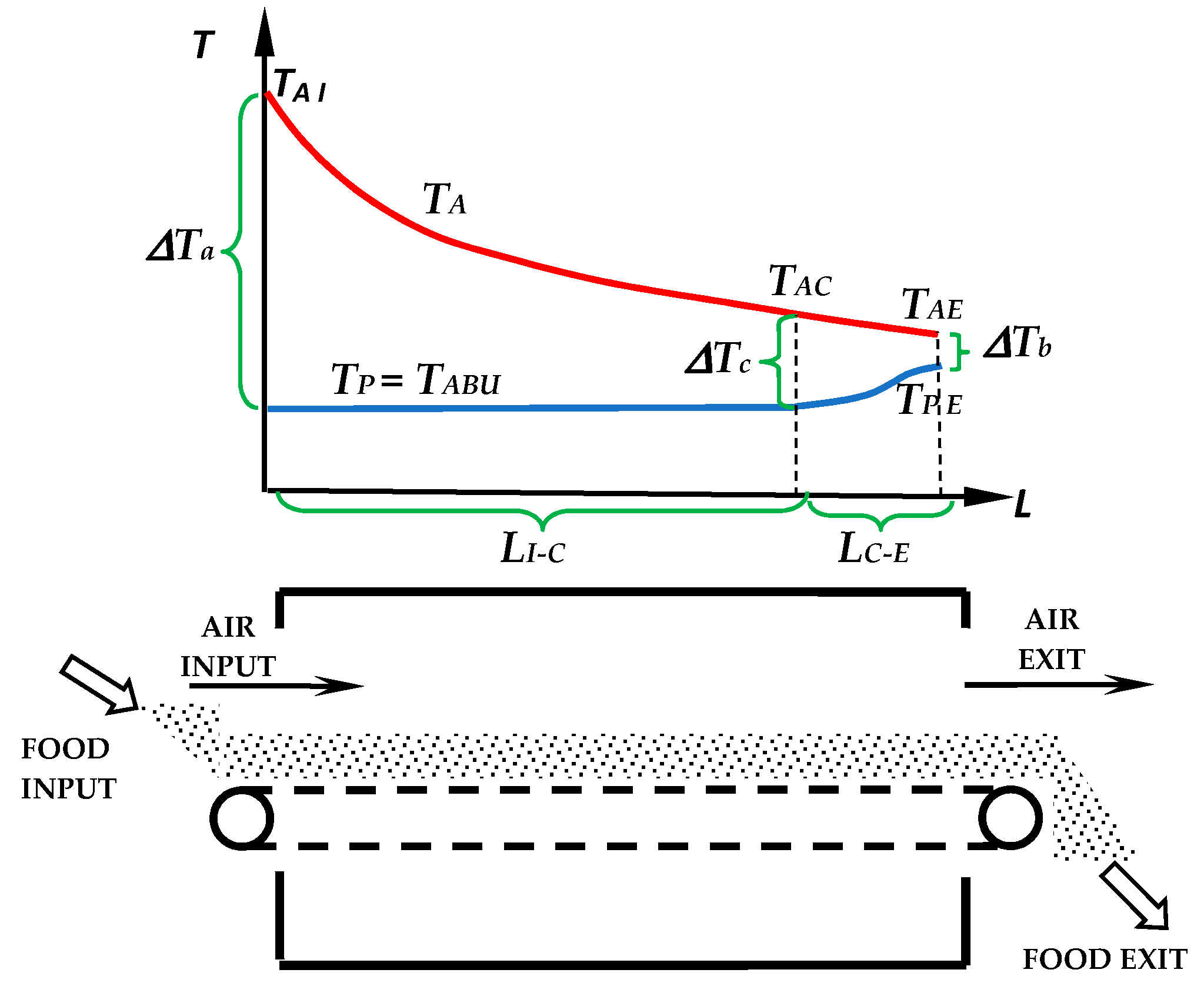
2.1.1. First Zone of the Dryer L_I-C

In the first zone, long L_I-C, the product is characterized by a moisture content X higher than the critical one X_C, and therefore it maintains its temperature T_P constant and equal to the wet bulb temperature T_WB [1]. In this first zone, the equations proposed in the previous work [1] are valid. The first equation, called (12) in [1], concerns the heat transfer rate q_I-C that the warm and dry air of initial mass flow rate G_AI releases when cooling from the input temperature T_AI to temperature T_AC corresponding to the achievement of critical moisture content (Figure 1):

$$q_{I-C}=G_{AI}·c_A\left(T_{AI}-T_{AC}\right)·\eta$$

(1)

where: c_A is the specific heat of dry air; η is the corrective coefficient introduced in [2] and related to the heat losses. For the pilot dryer used in the experiments performed in this work, η is equal to 0.965.

The second equation, called (13) in [1], concerns the heat transfer rate q_I-C exchanged between the air and the product:

$$q_{I-C}=\mathsf{\alpha }·A_{I-C}·\Delta T_{mL\left(I-C\right)}$$

where: α is the convective heat transfer coefficient; ΔT_mL(I-C) is the logarithmic mean temperature difference in the I-C zone; A_I-C is the total area of the product inside the I-C zone of the dryer.

From Equation (18) of [1]: $A_{I-C}=f·L_{I-C}$; where: f is the transverse dimension shown in Figure 5 of [1]; L_I-C is the length of the I-C zone of the dryer (Figure 1). Therefore, the equation that gives the heat transfer rate exchanged between air and product is:

$$q_{I-C}=\mathsf{\alpha }·f·L_{I-C}·\Delta T_{mL\left(I-C\right)}$$

(2)

The third equation refers to the heat transfer rate required by the water in the product to evaporate. It was indicated with the number (20) in [1]:

$$q_{I-C}=G_{EV\left(I-C\right)}·r_{I-C}=H_I·B_I·v_{Belt}·{\rho }_{BulkI}·\frac{X_I-X_C}{1+X_I}·r_{I-C}$$

(3)

where: G_EV(I-C) is the mass flow rate of the evaporated water in the I-C zone; H_I is the input height and B_I is the input width of the bulk product on the belt; v_Belt is the belt speed; ρ_BulkI is the bulk density of the input product; X_I is the input moisture content; X_C is the critical moisture content; r_I-C is the thermal energy, in the I-C zone, required to produce 1 kg of superheated steam at the air temperature T_A; r_I-C is equal to the difference in enthalpy [3] between the superheated steam at T_A and the water contained in the product to be dried at the temperature T_P. As indicated in [1] r_I-C is considered constant and has an average value of 2617 kJ kg⁻¹.

2.1.2. Second Zone of the Dryer L_C-E

In order to write the mathematical modelling of the C-E drying zone in which the product moisture content is lower than the critical one (X < X_C), the first equation proposed concerns the heat transfer rate q_C-E that the warm air of initial flow rate G_AI releases when cooling from the temperature T_AC to the exit temperature T_AE. This equation is similar to (1):

$$q_{c-E}=G_{AI}·c_A\left(T_{AC}-T_{AE}\right)·\eta$$

(4)

where: G_AI is the mass flow rate of drying air; c_A is its specific heat; η is the corrective coefficient introduced in [2], related to the heat losses and equal to 0.965 for the pilot dryer used in the experiments. The steam mass flow rate coming from the previous L_I-C dryer area and mixed with the air, has been neglected because analyzing the data indicated in [1] it is about 2% of the dry air flow rate G_AI and therefore two orders of magnitude less than G_AI.

The second equation, concerning the heat transfer rate q_C-E exchanged between air and product, is similar to (2):

$$q_{C-E}=\mathsf{\alpha }·f·L_{C-E}·\Delta T_{mL\left(C-E\right)}$$

(5)

where: α is the convective heat transfer coefficient; ΔT_mL(C-E) is logarithmic mean temperature difference in the C-E zone; f is the transverse dimension shown in Figure 5 of [1]; L_C-E is the length of the C-E zone of the dryer (Figure 1).

The third equation refers to the heat transfer rate q_C-E required by the water to evaporate and, similarly to (3), it is:

$$q_{C-E}=G_{EV\left(C-E\right)}·r_{C-E}=H_I·B_I·v_{Belt}·{\rho }_{BulkC}·\frac{X_C-X_F}{1+X_C}·r_{C-E}$$

(6)

where: G_EV(C-E) is the mass flow rate of the evaporated water in the C-E zone; H_I is the input height and B_I is the input width of the bulk product on the belt; v_Belt is the belt speed; ρ_BulkC is the bulk density in the point where the product has the critical moisture content; X_C is the critical moisture content; X_F is the final moisture content; r_C-E is the thermal energy, in the C-E zone, required to produce 1 kg of superheated steam at the air temperature T_A and is equal to the difference in enthalpy [3] between the superheated steam at T_A and the water contained in the product to be dried at the temperature T_P. The thermal energy r_C-E is currently unknown.

A fourth equation must be added to correlate the bulk density ρ_BulkC of the product at point C to the input bulk density ρ_BulkI.

Considering: ${\rho }_{BulkI}=\frac{m_D+m_{WI}}{V}$; and: ${\rho }_{BulkC}=\frac{m_D+m_{WC}}{V}$, where: m_D is the dry mass; m_W is the mass of water; V is the bulk volume; we obtain:

$$\frac{{\rho }_{BulkC}}{{\rho }_{BulkI}}=\frac{1+X_C}{1+X_I}$$

(7)

Finally, the L_C-E zone with X < X_C is characterized by a drying constrained to the process of internal diffusion of water towards the surface of the product. The diffusion of water inside the product is described by Fick’s second law, i.e., by a partial differential equation (PDE) that in the one-dimensional case is: $\frac{\partial X}{\partial t}=D\frac{{\partial }^2\mathrm{X}}{\partial y^2}$.

In the case of a simple geometry such as the thin plate to which many food products are similar and excluding the initial period corresponding to the phenomenon of delay, Perry [72] suggests a solution of the PDE, such as:

$$\frac{X-X_{eq}}{X_C-X_{eq}}=\frac{8}{{\pi }^2}{e}^{-\frac{D·{\pi }^2}{4·{\delta }^2}t}$$

(8)

where: X is the moisture content as a function of the drying time t; X_C is the critical moisture content of the product and corresponds to the initial one of the drying in the L_C-E zone; X_eq is the equilibrium moisture content; D is the mass diffusivity of water inside the product; δ is half the thickness of the plate.

By differentiating we obtain:

$$\frac{dX}{dt}=-\left(X_C-X_{eq}\right)·\frac{2D}{{\delta }^2}·e^{-\frac{D·{\pi }^2}{4·{\delta }^2}t}$$

(9)

Since [1]: $\frac{dX}{dt}=-\frac{G_{EV}}{m_D}$, where: G_EV is the instantaneous mass flow rate of evaporated water; m_D is the dry mass present in the L_C-E section of the dryer and is [2]: $m_D=\frac{H_I·B_I·{\rho }_{BulkC}·L_{C-E}}{1+X_C}$, that is, based on (7): $m_D=\frac{H_I·B_I·{\rho }_{BulkI}·L_{C-E}}{1+X_I}$. Furthermore, since the belt speed v_Belt is constant and: $v_{Belt}=\frac{z}{t}$, the previous (9) becomes:

$$G_{EV}=\frac{H_I·B_I·{\rho }_{BulkI}·L_{C-E}}{1+X_I}·\frac{2D}{{\delta }^2}·\left(X_C-X_{eq}\right)·e^{-\frac{D·{\pi }^2}{4·{\delta }^2·v_{Belt}}z}$$

(10)

This equation indicates that the mass flow rate of water evaporated G_EV varies along the horizontal coordinate z within the L_C-E zone of the dryer (Figure 1) according to the exponential function as shown in Figure 2.

Therefore, the integral average evaporated water flow rate G_EV(C-E) can be calculated as follows:

$$G_{EV\left(C-E\right)}=\frac{1}{L_{C-E}}{{\displaystyle \int }}_0^{L_{C-E}}\frac{H_I·B_I·{\rho }_{BulkI}·L_{C-E}}{1+X_I}·\frac{2D}{{\delta }^2}·\left(X_C-X_{eq}\right)·e^{-\frac{D·{\pi }^2}{4·{\delta }^2·v_{Belt}}z}dz$$

Then:

$$G_{EV\left(C-E\right)}=\frac{H_I·B_I·{\rho }_{BulkI}·v_{Belt}}{1+X_I}·\frac{8}{{\pi }^2}·\left(X_C-X_{eq}\right)·\left[1-e^{-\frac{D·{\pi }^2}{4·{\delta }^2·v_{Belt}}{L}_{C-E}}\right]$$

(11)

However, since food products do not always have the plate shape, the previous equation must be rewritten to make the mathematical model more general:

$$G_{EV\left(C-E\right)}=\frac{H_I·B_I·{\rho }_{BulkI}·v_{Belt}}{1+X_I}·C_1·\left(X_C-X_{eq}\right)·\left[1-e^{-\frac{C_2}{v_{Belt}}{L}_{C-E}}\right]$$

(12)

where: C₁ and C₂ are constants to be determined by experiments.

The heat flow rate required for this mass flow rate of evaporated water is:

$$q_{C-E}=\frac{H_I·B_I·{\rho }_{BulkI}·v_{Belt}}{1+X_I}·C_1·\left(X_C-X_{eq}\right)·\lceil 1-e^{-\frac{C_2}{v_{Belt}}{L}_{C-E}}\rceil ·r_{C-E}$$

(13)

Equation (13) is added to the other four Equations (4)–(7) to perform mathematical modelling of the drying in the L_C-E zone where the moisture content is X < X_C.

2.2. Design Guidelines

In the previous paragraph, eight equations were found, namely (1), (2), (3), (4), (5), (6), (7) and (13), in which there are eight unknowns: q_I-C, q_C-E, G_AI, ρ_BulkI, T_AC, L_I-C, L_C-E and T_PE. Therefore, this system of equations has a solution, which will be found in the next sub-paragraphs, where the design guidelines will be also proposed.

2.2.1. Air Temperature T_AC at Critical Moisture Content of the Product

Since the air temperature at the input T_AI and exit T_AE of the dryer can be imposed a priori [1], the combination of Equations (1) and (3) gives:

$$G_{AI}·c_A·\left(T_{AI}-T_{AC}\right)·\eta =H_I·B_I·v_{Belt}·{\rho }_{BulkI}·\frac{X_I-X_C}{1+X_I}·r_{I-C}$$

(14)

The combination of Equation (4) with (6) and (7) gives:

$$G_{AI}·c_A·\left(T_{AC}-T_{AE}\right)·\eta =H_I·B_I·v_{Belt}·{\rho }_{BulkI}·\frac{X_C-X_F}{1+X_I}·r_{C-E}$$

(15)

The division of (14) with (15), after a few steps, gives the T_AC temperature (Figure 1):

$$T_{AC}=\frac{T_{AE}·\left(X_I-X_C\right)·r_{I-C}+T_{AI}·\left(X_C-X_F\right)·r_{C-E}}{\left(X_I-X_C\right)·r_{I-C}+\left(X_C-X_F\right)·r_{C-E}}$$

(16)

The T_AC value allows us to calculate ΔT_c (Figure 1): $\Delta T_c=\left(T_{AC}-T_{WB}\right)$, where T_WB is the temperature of the product equal to the wet bulb temperature [1].

2.2.2. Length of Dryer L_I-C to Reach Critical Moisture Content X_C

The combination of Equation (2) with (3) and the observation [1] that $\frac{f·\alpha }{H_I·B_I}=F·\alpha$, where F is the form factor of the product, gives the length of the dryer L_I-C corresponding to the zone with X > X_C:

$$L_{I-C}=\frac{v_{Belt}·{\rho }_{BulkI}·r_{I-C}}{F·\alpha ·\Delta T_{mL\left(I-C\right)}}·\frac{X_I-X_C}{1+X_I}$$

(17)

Equation (17) is similar to (23) of [1].

2.2.3. Mass Flow Rate of Drying Air G_AI

The combination of Equation (1) with (3) gives the mass flow rate of drying air G_AI:

$$G_{AI}=\frac{B_I·H_I·v_{Belt}·{\rho }_{BulkI}}{c_A·\left(T_{AI}-T_{AC}\right)·\eta }·\frac{X_I-X_C}{1+X_I}·r_{I-C}$$

(18)

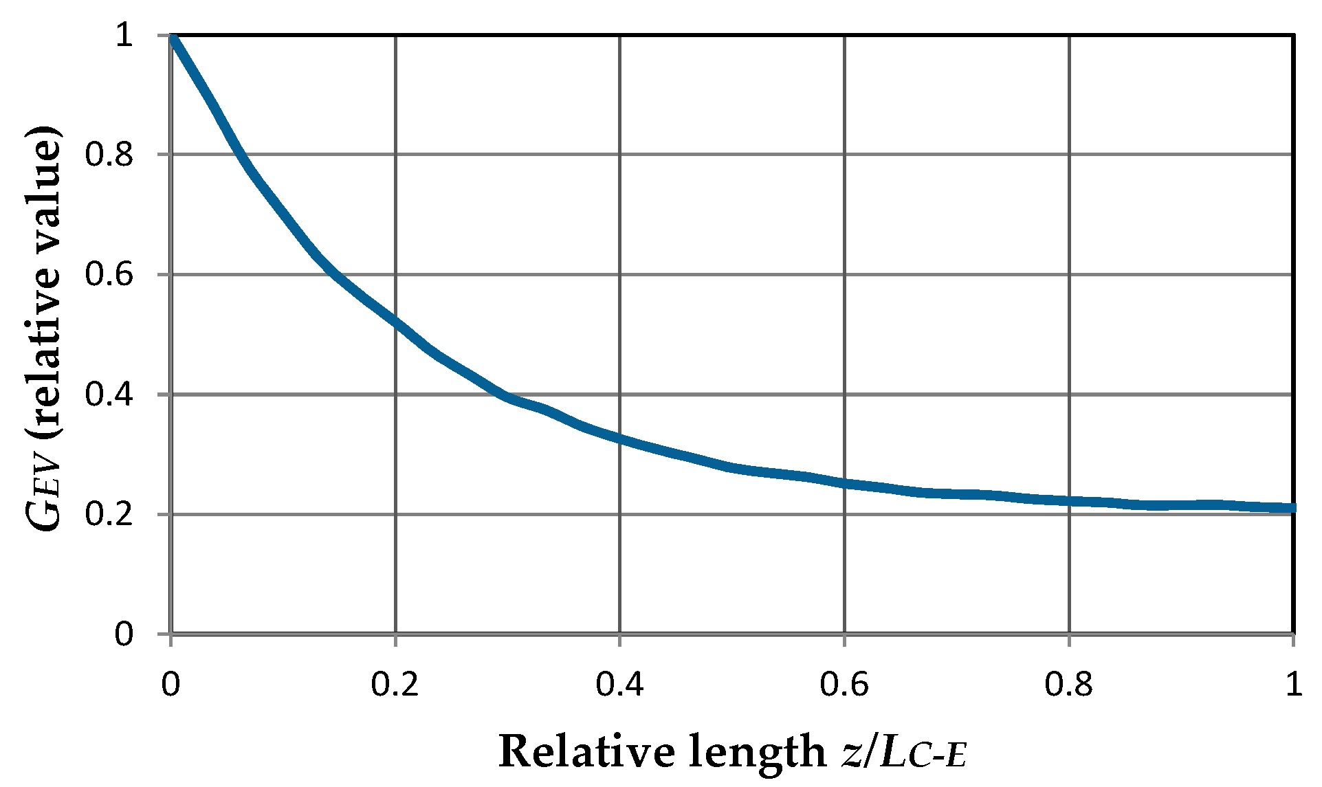
2.2.4. Length of Dryer L_C-E to Reduce Moisture Content from Critical Value X_C to Final One X_F

The combination of Equation (4) with (13), gives the length of the dryer L_C-E where the product dries from X_C to X_F:

$$L_{C-E}=-\frac{v_{Belt}}{C_2}·\ln \left[1-\frac{G_{AI}·c_A·\left(T_{AC}-T_{AE}\right)·\eta }{C_1·H_I·B_I·{\rho }_{BulkI}·v_{Belt}·r_{C-E}}·\frac{1+X_I}{X_C-X_{eq}}\right]$$

(19)

2.2.5. Temperature Difference Δt_b at the Dryer Exit and Product Exit Temperature T_PE

The combination of Equation (4) with (5) gives the temperature difference between the air and the product at the exit of the dryer (Figure 1): $\Delta T_b=T_{AE}-T_{PE}$, where T_AE is the air exit temperature and T_PE is the product exit temperature:

$$\Delta T_{mL\left(C-E\right)}=\frac{\Delta T_c-\Delta T_b}{\ln \frac{\Delta T_c}{·T_b}}=\frac{G_{AI}·c_A·\left(T_{AC}-T_{AE}\right)·\eta }{F·\mathsf{\alpha }·H_I·B_I·L_{C-E}}.$$

(20)

The temperature difference ΔT_b can be obtained by an iterative method easily through a spreadsheet. As seen in Section 2.2.1, the T_AE temperature can be set a priori and, therefore, the product exit temperature $T_{PE}=T_{AE}-\Delta T_b$ can be obtained.

2.2.6. Known Quantities and Experimental Quantities

• The input and exit temperatures of the drying air T_AI and T_AE can be defined using the guidelines 3.1.1 proposed in [1].
• The compound quantity F·α is the product of the convective heat transfer coefficient α and the form factor $F=\frac{f}{H_I·B_I}$, where f is the transverse dimension (Figure 5 in [1]) and H_I and B_I are the height and width of the bulk product placed above the belt, respectively. The quantity F·α is measured as indicated in the guidelines 3.1.9 of [1].
• The bulk density ρ_BulkI is measured as indicated in the next point I) of Section 2.3.
• The thermal energy r_I-C has an average value of 2617 kJ kg⁻¹, as indicated in guidelines 3.1.6 of [1].
• The constants C₁ and C₂, where the first one can be connected to the diffusivity of the water inside the product and to the size and the second concerns the initial delay, must be determined using the experimental method that will be described in the next Section 2.3. The same experimental method will also allow us to determine the critical moisture content X_C and the equilibrium moisture content X_eq.
• To determine the lengths L_I-C and L_C-E of the dryer, it is necessary to impose the belt speed v_Belt and the height H_I and the width B_I of the bulk product above the belt. These three quantities must be chosen a priori in order to reach the total mass flow rate of evaporated water G_EV(I-E) foreseen for the dryer. In fact, it is known that the quantity characterizing a dryer, both technically and commercially, is the G_EV(I-E) quantity. Therefore, the designer must start from: a known value of the mass flow rate G_EV(I-E); the input and final moisture content and from bulk density of the product; an equation obtained by adding the mass flow rate of evaporated water G_EV(I-C) in the L_I-C zone, and the one G_EV(C-E) of the L_C-E zone:

  $$G_{EV\left(I-E\right)}=G_{EV\left(I-C\right)}+G_{EV\left(C-E\right)}=H_I·B_I·v_{Belt}·{\rho }_{BulkI}\frac{X_I-X_F}{1+X_I}$$

  (21)

In this equation, the designer can choose the values of H_I, B_I and hence can obtain the v_Belt.

g.

Finally, the thermal energy r_C-E in the L_C-E length zone with X < X_C must be measured. The r_C-E will be greater than the r_I-C of the zone with X > X_C, since below a certain value of the moisture content X, lower than the critical one X_C, the evaporation of the bound water requires thermal energy greater than that for free-form water. In Section 2.3 the iterative method for determining the experimental values of r_C-E will be described.

2.3. Experimental Procedure and Equipment

The experimental activity was carried out using a pilot dryer. The pilot dryer was the same as in previous works [1,2] and

Table 1. Geometrical and operational data of the pilot dryer.

Quantity	Symbol	Value
Belt width	BI (m)	0.3
Total Belt length	LT (m)	6.0
Alfalfa bulk height	HI (m)	0.05
Flow section of the drying air	AA (m2)	0.15
Form factor·Convective heat transfer coefficient [1]	F·α (W·m−3·K−1)	5144

summarizes its geometrical data. All the tests were carried out by drying alfalfa consisting of leaves attached to the stems cut in pieces 5 cm long. In the table the value of the quantity F·α relative of alfalfa is also reported. This quantity F·α was experimentally evaluated in the previous work [1].

The measuring instruments used were: infrared thermometer for the alfalfa temperature; PT100 resistance thermometers for the input and exit temperature of the dryer; precision balance for weighing the sample before and after dehydration in an oven for two hours at 135 °C to measure the moisture content of the product at the input and exit; a pitot anemometer; data logger. The bulk density was calculated after measuring the mass and volume of the samples. Five replicates were made for each test.

The three purposes of the experiments were:

(I)

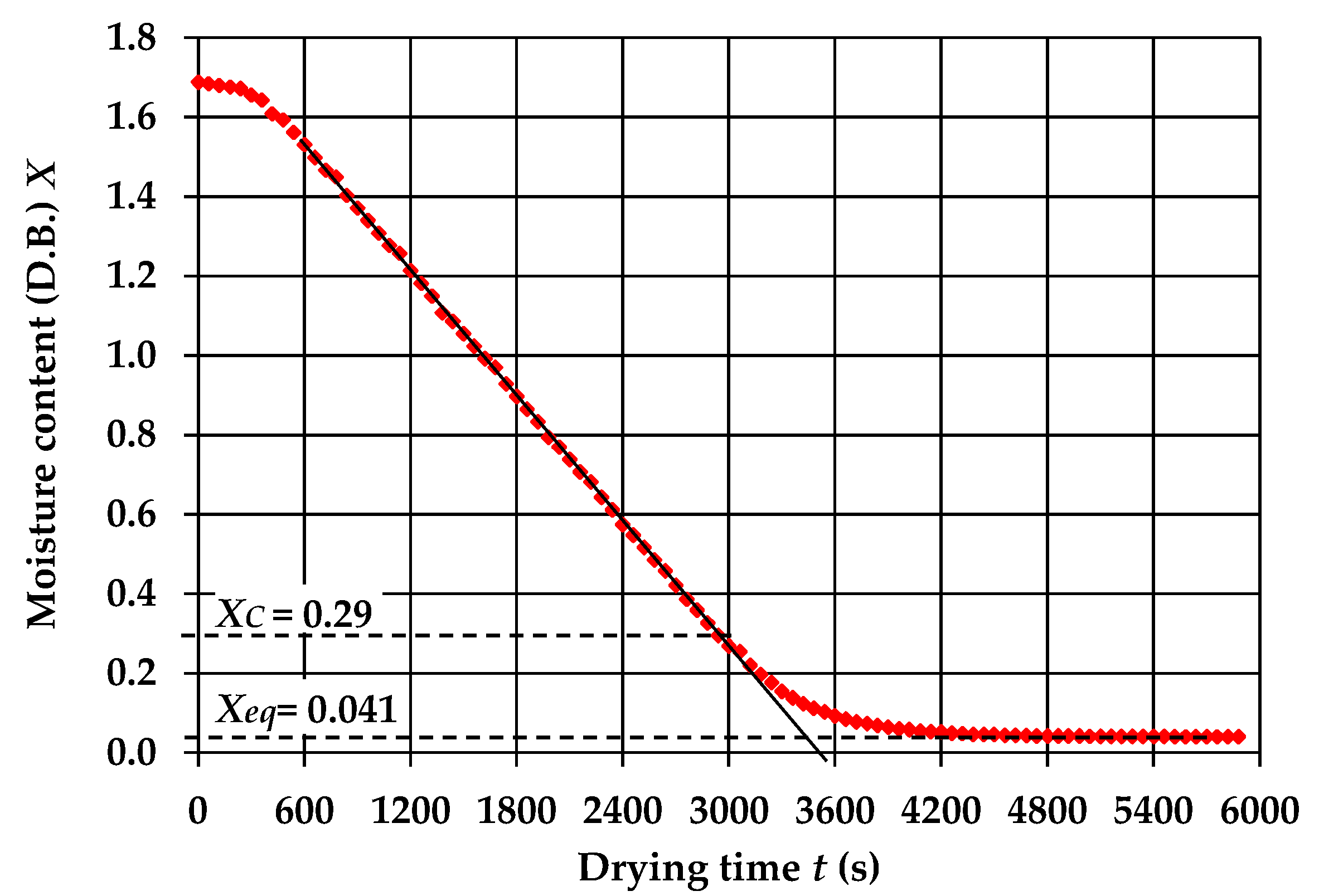
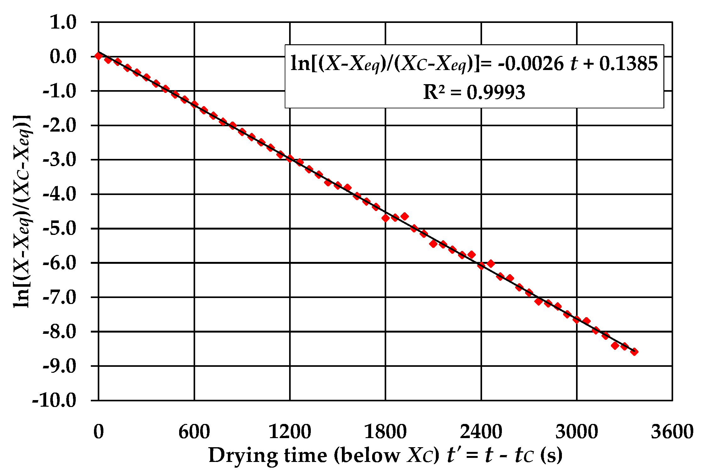
to quantify the constants C₁, C₂, the critical moisture content X_C and the equilibrium moisture content X_eq of the alfalfa were as foreseen in the previous point e. of Section 2.2.6. The four quantities, C₁, C₂, X_C and X_eq can be obtained from the experimental drying curve plotted in a diagram (time, moisture content), by interpolating the moisture content data measured each minute on a sample of the product inserted in the pilot dryer. The sample of alfalfa of initial moisture content X_I was placed with a height H_I equal to 0.05 m on a thin aluminum plate 1 m long and 0.3 m wide, i.e. like the dryer belt width. In turn, the plate was placed on a precision balance placed on the locked belt of the dryer. Only the drying air at the temperature T_AI equal to 60 °C was forced by the fan to lick the product sample. The total mass of the sample m_T = m_W + m_D, dry mass m_D plus water mass m_W, was measured each minute. Knowing [2] that $m_D=\frac{m_{TI}}{1+X_I}$, where m_TI is the initial mass of the sample, the moisture content X of the product at instant t in which the mass of the alfalfa sample m_T is measured, can be calculated as follows:

$$X=\frac{m_T}{m_D}-1=\frac{m_T}{m_{TI}}\left(1+X_I\right)-1$$

(22)

where the initial moisture content X_I is measured on a separate sample of the same alfalfa, by weighing the mass before and after drying in an oven at 135 ° C for two hours. Therefore, the drying curve plotted on the t-X diagram allows obtaining C₁, C₂, X_C and X_eq (see also the next Section 3);

(II)

to quantify the thermal energy r_C-E during drying with X<X_C by means of an iterative procedure as provided in point g. of the previous 2.2.6. The iterative procedure consists of three steps. In the first step, r_C-E is assumed equal to r_I-C that is 2617 kJ kg^-1 and a preliminary design of the dryer is performed according to guidelines 2.2. However, some guidelines are overturned because the pilot dryer already has a predetermined length L_T=L_I-C+L_C-E=6 m. Therefore, in this case the sequence of calculations is seen to impose L_T = 6 m to derive the belt speed v_Belt. For the rest of the quantities, the guidelines are the same as in Section 2.2, thus determining the air temperature T_AC and T_AE, the mass flow rate of the drying air G_AI and the product exit temperature T_PE, using equations in the Section 2.2.1, Section 2.2.3 and Section 2.2.5. The second step consists in carrying out a test on the pilot dryer functioning as required by the preliminary design. During the test, the actual temperatures T’_PE and T’_AE are measured, which will be different from those of the preliminary design T_PE and T_AE. The third step consists in looking for the r_C-E value which, inserted in the equations of guidelines 2.2, allows to restore the initial values of the T_PE and T_AE temperatures of the preliminary project, to the experimental values T’_PE and T’_AE. Since the equations of guidelines 2.2 are implementable in a spreadsheet, it is very easy to perform this third step;

(III)

to validate the mathematical model described in 2.1 and the design guidelines described in 2.2.

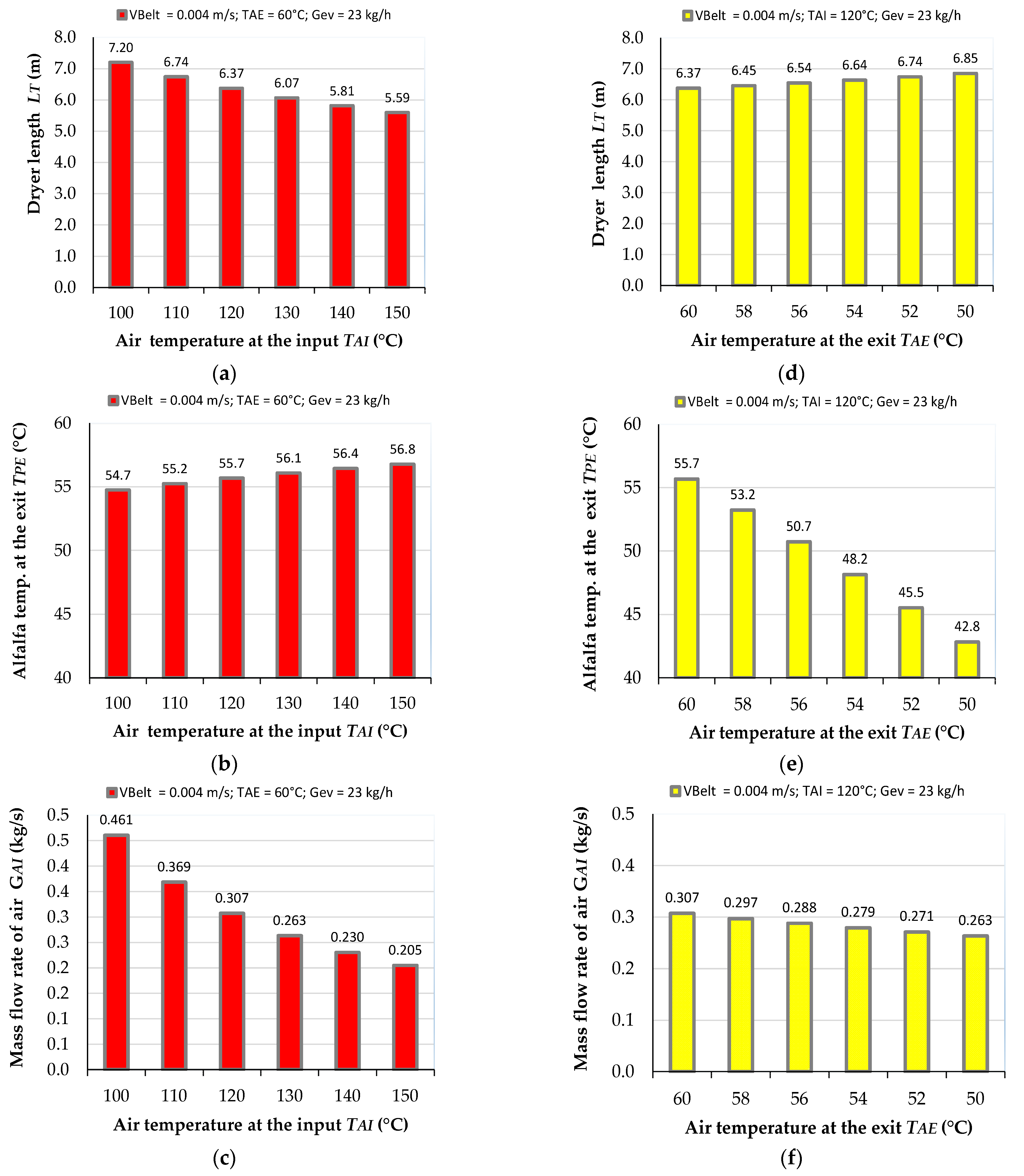
3. Results

To determine the quantities X_C, X_eq, C₁ and C₂, the series of tests was conducted as described in purpose (I) of the previous Section 2.3. Figure 3 shows the time-moisture content diagram (t-X) called drying curve. The value of the critical moisture content X_C was measured at the point where the straight section, which represents the drying phase at constant rate (dX/dt = R_C), begins to flex, exactly when the derivative dX/dt changes by 1% with respect to the value of the slope of the line equal to R_C.

When the measured moisture content value remained constant for five consecutive readings (5 min), it was defined as the equilibrium moisture content X_eq.

To determine the constants C₁ and C₂, the diagram of Figure 4 was made using data of Figure 3 relating to the phase with decreasing drying rate, i.e., for X ≤ X_C. In fact, the time on the abscissa is t’ = t − t_C, where t_C is the time to reach the critical moisture content X_C. In ordinate there is the quantity: $\ln \left(\frac{X-X_{eq}}{X_C-X_{eq}}\right).$

Starting from Equation (13) and returning to having time as an independent variable, it becomes:

$$\ln \frac{X-X_{eq}}{X_C-X_{eq}}=\ln C_1-C_2·t$$

(22)

This is the equation of a line that has a negative slope equal to −C₂ and intercept equal to ln(C₁), therefore it is sufficient to look for the regression line in the diagram of Figure 4, to obtain ln(C₁) = 0.1385 and C₂ = 0.0026.

Table 2. Results from experimental drying curve.

Quantity	Symbol	Value
Alfalfa input moisture content (D.B.)	XI	1.688 ± 0.105
Alfalfa input bulk density	ρBulkI (kg·m−3)	183 ± 7.6
Alfalfa critical moisture content (D.B.)	XC	0.290
Alfalfa equilibrium moisture content (D.B.)	Xeq	0.041
Coefficient related to delay	C1	1.149
Coefficient related to diffusivity	C2	0.0026

summarizes the results obtained.

To determine the average thermal energy r_C-E required to evaporate 1 kg of water during drying with X < X_C, the procedure adopted is that described in purpose II) of the previous Section 2.3. The results of the three steps are indicated in

Table 3. Results of the three steps to obtain the thermal energy r_C-E concerning the humidity X < X_C. The first step refers to the results of the preliminary design with r_C-E equal to r_I-C = 2617 kJ/kg. The second step concerns the experimental measurement of moisture content and temperatures of the air and of the product (red font). The third step concerns the r_C-E value found (red font) through the equations of the design guidelines 2.3 by imposing the experimental temperatures (red font).

Quantity	Symbol	1st Step Preliminary Design	2nd Step Exper. Value	3rd Step Search for rC-E
Thermal energy	rC-E (kJ kg−1)	2617		4271
Input moisture content	XI	1.688	1.688 ± 0.105	1.688
Final moisture content	XF	0.122	0.121 ± 0.01	0.122
Input bulk density	ρBulkI (kg m−3)	183	183 ± 7.6	183
Critical moisture content	XC	0.290	=	0.290
Equilibrium moisture content	Xeq	0.041	=	0.041
Air input temperature	TAI (°C)	120	119.7 ± 1.2	120
Air exit temperature	TAE (°C)	57	52.7 ± 1.1	52.7
Belt velocity	vBelt (m s−1)	0.0036	=	0.0036
Air temperature in C	TAC (°C)	63.8	=	63.8
Dryer length I-C (Figure 1)	LI-C (m)	3.55	=	3.55
Dryer length C-E (Figure 1)	LC-E (m)	2.45	=	2.45
Total dryer length	LT (m)	6.00	=	6.00
Product exit temperature	TPE (°C)	55.6	46.5 ± 0.7	46.5
Air input mass flow rate	GAI (kg s−1)	0.246	0.246 ± 0.006	0.246

.

During the first step, the dryer was preliminarily designed by imposing a thermal energy in the C-E section, where X < X_C, r_C-E is 2617 kJ/kg, i.e., the same as in the I-C section, where X > X_C. In addition, a total length L_T equal to 6 m was set for this preliminary design, which is the length of the pilot dryer (Table 1), in order to obtain the belt speed v_Belt, through the design guidelines of Section 2.2. Instead, the belt speed v_Belt is normally chosen, so that the mass flow rate of evaporated water G_EV(I-E) foreseen for the dryer is satisfied through Equation (21), and consequently, through the design guidelines 2.2, the length L_T is calculated.

Therefore, the data of the first column (first step) are related to this preliminary design (blue font). In the second step, it was planned to carry out the experimental survey on the pilot dryer, running with the data obtained in the first step. Among the experimental measurements detected, the most important were the product exit temperature T_PE (red font) and the air exit temperature T_AE (red font). As reported in the second column (2nd step) of Table 3, the values of these quantities are lower than those expected from the preliminary design: an experimental T’_AE = 52.7 °C instead of design T_AE = 57 °C and an experimental T’_PE = 46.5 °C instead of design T_PE = 55.6 °C. It is clear the experimental T’_AE lower than the design T_AE indicates that the air has more cooled to transmit a greater heat flow rate towards the product to be dried. This is an indication that the product requires a thermal energy r_C-E greater than that assumed in the preliminary design, which was 2617 kJ kg⁻¹. The decrease in the experimental T’_PE compared to the design T_PE can also be explained by the need to transmit a greater heat flow rate to the product due to r_C-E greater than 2617 kJ kg⁻¹. In fact, the experimental T’_PE settled on a value that produced a logarithmic mean temperature difference ΔT’_mL(C-E) of Equation (5) equal to 13.9 °C against the 8.5 °C of the ΔT_mL(C-E) calculated during the design of the first step. Therefore, the increase in ΔT_mL(C-E) is 63.2% and implies that the heat flow rate q_C-E has to increase by the same amount based on Equation (5), therefore based on Equation (6) also the thermal energy r_C-E has to increase by 63.2% i.e., from 2617 to 4271 kJ kg⁻¹. This last value coincides with that obtained in the third step (Table 3) according to the procedure of purpose (II) of Section 2.3, confirming that the calculations are correct.

The purpose (III) of the experiments, described in Section 2.3, concerned the validation of the mathematical modelling 2.1 and of the design guidelines 2.2, using the value of the thermal energy r_C-E equal to 4271 kJ kg⁻¹ as just determined. For a broader validation, the experiments were doubled with the air input temperature T_AI set on two values: 120 °C and 100 °C.

Table 4. Results of the validation of the mathematical modeling and design guidelines.

Quantity	Symbol	Design	Exper. Value	Design	Exper. Value
Air input temperature	TAI (°C)	120	119.7 ± 1.2	100	100.9 ± 1.1
Thermal energy (X > XC)	rI-C (kJ kg−1)	2617	=	2617	=
Thermal energy (X < XC)	rC-E (kJ kg−1)	4271	=	4271	=
Input moisture content	XI	1.688	1.688 ± 0.105	1.688	1.688 ± 0.105
Final moisture content	XF	0.122	0.120 ± 0.01	0.122	0.124 ± 0.009
Input bulk density	ρBulkI (kg m−3)	183	183 ± 7.6	183	183 ± 7.6
Critical moisture content	XC	0.290	=	0.290	=
Equilibrium moisture content	Xeq	0.041	=	0.041	=
Air exit temperature	TAE (°C)	57	56.7 ± 1.0	57	56.8 ± 0.9
Belt velocity	vBelt (m s−1)	0.00369	=	0.00344	=
Air temperature in C	TAC (°C)	67.3	66.9 ± 0.9	64.1	64.3 ± 0.8
Dryer length I-C (Figure 1)	LI-C (m)	3.47	=	3.64	=
Dryer length C-E (Figure 1)	LC-E (m)	2.53	=	2.36	=
Total dryer length	LT (m)	6.00	=	6.00	=
Product exit temperature	TPE (°C)	52	52.4 ± 0.6	52.1	52.2 ± 0.7
Air input mass flow rate	GAI (kg s−1)	0.270	0.269 ± 0.006	0.368	0.369 ± 0.005
Evaporated water flow rate	GEV (kg s−1)	0.00591	=	0.00550	=

shows the results obtained. The values of the quantities in the first column are those of the design carried out according to guidelines 2.3 with T_AI equal to 120 °C. The values of the second column are those detected during the test with T_AI equal to 120 °C and concern: the product moisture content at the input X_I and at the exit X_F; the input bulk density ρ_BulkI; the air exit temperature T_AE; the air temperature T_AC at point C (Figure 1); the product exit temperature T_PE. All the other quantities of the first column (design), particularly the length of the dryer L_T, the mass air flow rate G_AI and the speed of the belt v_Belt resulted in the same value also during the test (second column) due to the adjustments imposed on the pilot dryer.

The third and fourth columns are similar to the first and second respectively, but with air input temperature T_AI equal to 100 °C.

For both T_AI of 120 °C and 100 °C, there were no significant differences between the experimental values and the expected ones from the design on: the air exit temperatures T_AE; the product exit temperatures T_PE; the air temperatures T_AC in point C of Figure 1. Even the product exit moisture content X_F did not show significant differences between the experimental values and those expected from the design.

As consequence of these positive results validating mathematical modelling 2.1 and design guidelines 2.2, a part of the equations of the model can be used to extend a result that was obtained in the previous work [2]. In [2], an equation was obtained, numbered (12), which correlated the final moisture content X_F to the air exit temperature T_AE, valid for final moisture content greater than the critical one (X_F > X_C). In this way, it was possible to indicate the indirect measurement of the final moisture content X_F, useful for optimized adjustment of the drying operation, through the simpler, faster and cheaper measurement of the air exit temperature T_AE. Therefore, with the validated equations of the mathematical modelling of Section 2.1 proposed for drying with final moisture content lower than the critical one (X_F < X_C), the comparison between (1), (3), (4), (6) and (7) gives the following equation in place of (12) of [2]:

$$X_F=X_C+\left(X_I-X_C\right)\frac{r_{I-C}}{r_{C-E}}+\frac{G_{AI}·c_A·\left(1+X_I\right)}{B_I·H_I·v_{Belt}·{\rho }_{BulkI}·r_{I-C}}·\left(T_{AE}-T_{AI}\right)·\eta$$

(24)

Knowing the critical moisture content of the product X_C, its input moisture content X_I, its bulk density ρ_BulkI, its bulk dimensions on the belt B_I and H_I, the thermal energy values r_I-C and r_C-E, the mass flow rate of air G_AI, its input temperature T_AI, the belt speed v_Belt and by measuring the air exit temperature T_AE, Equation (24) shows that the final moisture content X_F is promptly obtained. The same equation, appropriately implemented in a PLC, suggests how to correct the X_F, if this is not the expected value, for example by changing the belt speed v_Belt, or the air input temperature T_AI.

The last result concerns a simulation using the equations of the design guidelines. The influence of the air temperature at the input T_AI on the following three variables was analyzed: the length of the dryer L_T; the product temperature at the exit T_PE; the mass flow rate of drying air G_AI. Since this air temperature at the input T_AI is chosen by the designer within a range that depends on the nature of the product [1], the simulation has highlighted the influence of this choice on the three variables defined above. The series of diagrams on the left of Figure 5a–c represents the trend of the three variables as a function of T_AI which has values between 100 °C and 150 °C. During the simulation, the following quantities were kept constant: the belt speed v_Belt equal to 0.004 m s⁻¹; the air temperature at the exit T_AE equal to 60 °C; the mass flow rate of evaporated water in the dryer G_EV equal to 23 kg h⁻¹. It is noted that the dryer length decreases significantly. This positive effect is reflected in a more compact system, but there is a slight increase in the product temperature at the exit T_PE, by just a couple of degrees, which is therefore acceptable, and a reduction in the mass flow rate of drying air G_AI to keep the mass flow rate of evaporated water G_EV constant given the increase by T_AI. Therefore, the space problem that afflicts these dryers can be mitigated with an increase in T_AI.

The series of diagrams on the right of Figure 5d–f provides the three variables—length L_T, temperature T_PE, mass flow rate G_AI—vs. the air temperature at the exit T_AE which is reduced from 60 °C to 50 °C, keeping constant: the belt speed v_Belt equal to 0.004 m s⁻¹; the air temperature at the input T_AI equal to 120 °C; the mass flow rate of evaporated water in the dryer G_EV equal to 23 kg h⁻¹. The figure shows a slight increase in the length of dryer L_T of about 0.5 m (+8%), an important decrease of the product temperature at the exit T_PE which decreases from 55.7 °C to 42.8 °C improving the organoleptic and nutritional quality. It should be remembered that the product temperature T_P remains at the wet bulb temperature T_WB up to point C (Figure 1) which is located at about 4 m from the input of the dryer. Only in the last 2.75 m, where the moisture content of the product is below the critical one, does the temperature slowly rise up to T_PE.

4. Conclusions

In the food industry, the drying operation is still very widespread with the use of various types of system. In this work, the focus was on the conveyor-belt dryer with tangential flow that is underused because it is more cumbersome and more difficult to design, but it has the advantage of greater respect for heat-sensitive food products and, therefore, greater diffusion in the future it may be able to improve food quality. This is the dryer already studied in two previous works [1,2] for the case of final moisture content higher than critical moisture content (X_F > X_C). In this work, the mathematical modelling and design guidelines have been extended to the more general situation of a final moisture content lower than the critical one (X_F < X_C).

First, all the equations of the thermo-hygrometric exchange have been set up. The associated mathematical modelling allowed us to define design guidelines and also a method to calculate the thermal energy r_C-E, necessary to evaporate the water when the moisture content is lower than the critical one (X < X_C). In fact, it is always greater than that for X > X_C since starting from a certain moisture content below the critical one X_C, there is bound water which requires higher energy to evaporate compared to latent heat.

Among the eight equations of the mathematical modelling there is one describing the diffusion phenomenon of water inside the product when the moisture content of the product X is lower than the critical one X_C. The mathematical modelling and the equations for the design guidelines, including the method for calculating the thermal energy r_C-E, have been experimentally confirmed.

A part of the equations of the mathematical modelling presented here in Section 2.1 was also used to extend the result obtained in a previous work [2] dedicated to drying with the final moisture content of the product exceeding the critical one, X_F > X_C. It was an equation that correlated the air exit temperature T_AE with the final moisture content of the product X_F which needs to be known promptly and continuously during the operation of the dryer for the optimization and reduction of energy consumption [73] and for the control of thermal damage to the dried product.

Therefore, among the results of this work there is also the new equation extended to the case X_F < X_C, able to link the final moisture content X_F to the air exit temperature T_AE. If the equation is implemented in a dryer adjustment PLC, it will be able to keep the X_F value constant and optimized, controlling the T_AE which is much easier, faster and less expensive to detect than direct methods for measuring the X_F.

Finally, the mathematical modelling and equations of the design guidelines were used to simulate the influence of air temperatures at the input T_AI and, respectively, at the exit T_AE. This last analysis showed that by reducing the mass flow rate of drying air G_AI, with the same T_AI, the temperature T_AE and consequently the exit temperature of the product T_PE can be reduced with, consequently, less thermal damage to food.

References

1. Friso, D. Conveyor-belt dryers with tangential flow for food drying: Mathematical modeling and design guidelines for final moisture content higher than the critical value. Inventions 2020, 5, 22. [Google Scholar] [CrossRef]
2. Friso, D. Conveyor-Belt Dryers with Tangential Flow for Food Drying: Development of Drying ODEs Useful to Design and Process Adjustment. Inventions 2021, 6, 6. [Google Scholar] [CrossRef]
3. Geankopolis, C.J. Transport Process Unit Operations, 3rd ed.; Prentice-Hall International: Englewood Cliffs, NJ, USA, 1993; pp. 520–562. [Google Scholar]
4. Salemović, D.R.; Dedić, A.D.; Ćuprić, N.L. Two-dimensional mathematical model for simulation of the drying process of thick layers of natural materials in a conveyor-belt dryer. Therm. Sci. 2017, 21, 1369–1378. [Google Scholar] [CrossRef] [Green Version]
5. Salemović, D.R.; Dedić, A.D.; Ćuprić, N.L. A mathematical model and simulation of the drying process of thin layers of potatoes in a conveyor-belt dryer. Therm. Sci. 2015, 19, 1107–1118. [Google Scholar] [CrossRef]
6. Xanthopoulos, G.; Okoinomou, N.; Lambrinos, G. Applicability of a single-layer drying model to predict the drying rate of whole figs. J. Food Eng. 2017, 81, 553–559. [Google Scholar] [CrossRef]
7. Khankari, K.K.; Patankar, S.V. Performance analysis of a double-deck conveyor dryer—A computational approach. Dry. Technol. 1999, 17, 2055–2067. [Google Scholar] [CrossRef]
8. Kiranoudis, C.T.; Maroulis, Z.B.; Marinos-Kouris, D. Dynamic Simulation and Control of Conveyor-Belt Dryers. Dry. Technol. 1994, 12, 1575–1603. [Google Scholar] [CrossRef]
9. Pereira de Farias, R.; Deivton, C.S.; de Holanda, P.R.H.; de Lima, A.G.B. Drying of Grains in Conveyor Dryer and Cross Flow: A Numerical Solution Using Finite-Volume Method. Rev. Bras. Prod. Agroind. 2004, 6, 1–16. [Google Scholar] [CrossRef]
10. Kiranoudis, C.T.; Markatos, N.C. Pareto design of conveyor-belt dryers. J. Food Eng. 2000, 46, 145–155. [Google Scholar] [CrossRef]
11. Friso, D. A Mathematical Solution for Food Thermal Process Design. Appl. Math. Sci. 2015, 9, 255–270. [Google Scholar] [CrossRef]
12. Askari, G.R.; Emam-Djomeh, Z.; Mousavi, S.M. Heat and mass transfer in apple cubes in a microwave-assisted fluidized bed drier. Food Bioprod. Process. 2013, 91, 207–215. [Google Scholar] [CrossRef]
13. Ben Mabrouk, S.; Benali, E.; Oueslati, H. Experimental study and numerical modelling of drying characteristics of apple slices. Food Bioprod. Process. 2012, 90, 719–728. [Google Scholar] [CrossRef]
14. Esfahani, J.A.; Vahidhosseini, S.M.; Barati, E. Three-dimensional analytical solution for transport problem during convection drying using Green’s function method (GFM). Appl. Therm. Eng. 2015, 85, 264–277. [Google Scholar] [CrossRef]
15. Esfahani, J.A.; Majdi, H.; Barati, E. Analytical two-dimensional analysis of the transport phenomena occurring during convective drying: Apple slices. J. Food Eng. 2014, 123, 87–93. [Google Scholar] [CrossRef]
16. Golestani, R.; Raisi, A.; Aroujalian, A. Mathematical modeling on air drying of apples considering shrinkage and variable diffusion coefficient. Dry. Technol. 2013, 31, 40–51. [Google Scholar] [CrossRef]
17. Jokiel, M.; Bantle, M.; Kopp, C.; Halvorsen Verpe, E. Modelica-based modelling of heat pump-assisted apple drying for varied drying temperatures and bypass ratios. Therm. Sci. Eng. Prog. 2020, 19, 100575. [Google Scholar] [CrossRef]
18. Bon, J.; Rossellò, C.; Femenia, A.; Eim, V.; Simal, S. Mathematical modeling of drying kinetics for Apricots: Influence of the external resistance to mass transfer. Dry. Technol. 2007, 25, 1829–1835. [Google Scholar] [CrossRef]
19. Baini, R.; Langrish, T.A.G. Choosing an appropriate drying model for intermittent and continuous drying of bananas. J. Food Eng. 2007, 79, 330–343. [Google Scholar] [CrossRef]
20. Da Silva, W.P.; Silva, C.M.D.P.S.; Gomes, J.P. Drying description of cylindrical pieces of bananas in different temperatures using diffusion models. J. Food Eng. 2013, 117, 417–424. [Google Scholar] [CrossRef]
21. Da Silva, W.P.; Hamawand, I.; Silva, C.M.D.P.S. A liquid diffusion model to describe drying of whole bananas using boundary-fitted coordinates. J. Food Eng. 2014, 137, 32–38. [Google Scholar] [CrossRef]
22. Macedo, L.L.; Vimercati, W.C.; da Silva Araújo, C.; Saraiva, S.H.; Teixeira, L.J.Q. Effect of drying air temperature on drying kinetics and physicochemical characteristics of dried banana. J. Food Process Eng. 2020, 43, e13451. [Google Scholar] [CrossRef]
23. Kumar, P.S.; Nambi, E.; Shiva, K.N.; Vaganan, M.M.; Ravi, I.; Jeyabaskaran, K.J.; Uma, S. Thin layer drying kinetics of Banana var. Monthan (ABB): Influence of convective drying on nutritional quality, microstructure, thermal properties, color, and sensory characteristics. J. Food Process Eng. 2019, 42, e13020. [Google Scholar] [CrossRef]
24. Mahapatra, A.; Tripathy, P.P. Modeling and simulation of moisture transfer during solar drying of carrot slices. J. Food Process Eng. 2018, 41, e12909. [Google Scholar] [CrossRef]
25. Thayze, R.B.P.; Pierre, C.M.; Vansostenes, A.M.D.M.; Jacqueline, F.D.B.D.; Daniel, C.D.M.C.; Vital, A.B.D.O.; Iran, R.D.O.; Antonio, G.B.D.L. On the study of osmotic dehydration and convective drying of cassava cubes. Defect Diffus. Forum 2021, 407, 87–95. [Google Scholar] [CrossRef]
26. Ramsaroop, R.; Persad, P. Determination of the heat transfer coefficient and thermal conductivity for coconut kernels using an inverse method with a developed hemispherical shell model. J. Food Eng. 2012, 110, 141–157. [Google Scholar] [CrossRef]
27. Corzo, O.; Bracho, N.; Pereira, A.; Vàsquez, A. Application of correlation between Biot and Dincer numbers for determining moisture transfer parameters during the air drying of coroba slices. J. Food Process. Preserv. 2009, 33, 340–355. [Google Scholar] [CrossRef]
28. Ferreira, J.P.L.; Queiroz, A.J.M.; de Figueirêdo, R.M.F.; da Silva, W.P.; Gomes, J.P.; Santos, D.D.C.; Silva, H.A.; Rocha, A.P.T.; de Paiva, A.C.C.; Chaves, A.D.C.G.; et al. Utilization of cumbeba (Tacinga inamoena) residue: Drying kinetics and effect of process conditions on antioxidant bioactive compounds. Foods 2021, 10, 788. [Google Scholar] [CrossRef] [PubMed]
29. Khan, M.A.; Moradipour, M.; Obeidullah, M.; Quader, A.K.M.A. Heat and mass transport analysis of the drying of freshwater fishes by a forced convective air-dryer. J. Food Process Eng. 2021, 44, e13574. [Google Scholar] [CrossRef]
30. Osae, R.; Essilfie, G.; Alolga, R.N.; Bonah, E.; Ma, H.; Zhou, C. Drying of ginger slices. Evaluation of quality attributes, energy consumption, and kinetics study. J. Food Process Eng. 2020, 43, e13348. [Google Scholar] [CrossRef]
31. Elmas, F.; Varhan, E.; Koç, M. Drying characteristics of jujube (Zizyphus jujuba) slices in a hot air dryer and physicochemical properties of jujube powder. J. Food Meas. Charact. 2019, 13, 70–86. [Google Scholar] [CrossRef]
32. Kaya, A.; Aydin, O.; Dincer, I. Experimental and numerical investigation of heat and mass transfer during drying of Hayward kiwi fruits (Actinidia Deliciosa Planch). J. Food Eng. 2008, 88, 323–330. [Google Scholar] [CrossRef]
33. Akdas, S.; Baslar, M. Dehydration and degradation kinetics of bioactive compounds for mandarin slices under vacuum and oven drying conditions. J. Food Process. Preserv. 2015, 39, 1098–1107. [Google Scholar] [CrossRef]
34. Barati, E.; Esfahani, J.A. A new solution approach for simultaneous heat and mass transfer during convective drying of mango. J. Food Eng. 2011, 102, 302–309. [Google Scholar] [CrossRef]
35. Corzo, O.; Bracho, N.; Alvarez, C.; Rivas, V.; Rojas, Y. Determining the moisture transfer parameters during the air-drying of mango slices using biot-dincer numbers correlation. J. Food Process. Eng. 2008, 31, 853–873. [Google Scholar] [CrossRef]
36. Janjai, S.; Lamlert, N.; Intawee, P.; Mahayothee, B.; Haewsungcharern, M.; Bala, B.K.; Müller, J. Finite element simulation of drying of mango. Biosyst. Eng. 2008, 99, 523–531. [Google Scholar] [CrossRef]
37. Villa-Corrales, L.; Flores-Prieto, J.J.; Xamàn-Villasenor, J.P.; García-Hernàndez, E. Numerical and experimental analysis of heat and moisture transfer during drying of Ataulfo mango. J. Food Eng. 2010, 98, 198–206. [Google Scholar] [CrossRef]
38. Kouhila, M.; Moussaoui, H.; Lamsyehe, H.; Tagnamas, Z.; Bahammou, Y.; Idlimam, A.; Lamharrar, A. Drying characteristics and kinetics solar drying of Mediterranean mussel (mytilus galloprovincilis) type under forced convection. Renew. Energ. 2020, 147, 833–844. [Google Scholar] [CrossRef]
39. Taghinezhad, E.; Kaveh, M.; Jahanbakhshi, A.; Golpour, I. Use of artificial intelligence for the estimation of effective moisture diffusivity, specific energy consumption, color and shrinkage in quince drying. J. Food Process Eng. 2020, 43, e13358. [Google Scholar] [CrossRef]
40. Lemus-Mondaca, R.A.; Zambra, C.E.; Vega-Gàlvez, A.; Moraga, N.O. Coupled 3D heat and mass transfer model for numerical analysis of drying process in papaya slices. J. Food Eng. 2013, 116, 109–117. [Google Scholar] [CrossRef]
41. Guiné, R.P. Pear drying: Experimental validation of a mathematical prediction model. Food Bioprod. Process. 2008, 86, 248–253. [Google Scholar] [CrossRef]
42. Singh, P.; Talukdar, P. Design and performance evaluation of convective drier and prediction of drying characteristics of potato under varying conditions. Int. J. Therm. Sci. 2019, 142, 176–187. [Google Scholar] [CrossRef]
43. Pereira, J.C.A.; da Silva, W.P.; Gomes, J.P.; Queiroz, A.J.M.; de Figueiredo, R.M.F.; de Melo, B.A.; Santiago, A.M.; de Lima, A.G.B.; de Macedo, A.D.B. Continuous and intermittent drying of rough rice: Effects on process effective time and effective mass diffusivity. Agriculture 2020, 10, 282. [Google Scholar] [CrossRef]
44. Sabarez, H.T. Mathematical modeling of the coupled transport phenomena and color development: Finish drying of trellis-dried sultanas. Dry. Technol. 2014, 32, 578–589. [Google Scholar] [CrossRef]
45. Moussaoui, H.; Idlimam, A.; Lamharrar, A. The characterization and modeling kinetics for drying of taraxacum officinale leaves in a thin layer with a convective solar dryer. Lect. Notes Electr. Eng. 2019, 519, 656–663. [Google Scholar] [CrossRef]
46. Obajemihi, O.I.; Olaoye, J.O.; Cheng, J.-H.; Ojediran, J.O.; Sun, D.-W. Optimization of process conditions for moisture ratio and effective moisture diffusivity of tomato during convective hot-air drying using response surface methodology. J. Food Process Preserv. 2021, 45, e15287. [Google Scholar] [CrossRef]
47. Obajemihi, O.I.; Olaoye, J.O.; Ojediran, J.O.; Cheng, J.-H.; Sun, D.W. Model development and optimization of process conditions for color properties of tomato in a hot-air convective dryer using box–behnken design. J. Food Process Preserv. 2020, 44, e14771. [Google Scholar] [CrossRef]
48. Taghinezhad, E.; Kaveh, M.; Szumny, A. Optimization and prediction of the drying and quality of turnip slices by convective-infrared dryer under various pretreatments by rsm and anfis methods. Foods 2021, 10, 284. [Google Scholar] [CrossRef]
49. Castro, A.M.; Mayorga, E.Y.; Moreno, F.L. Mathematical modelling of convective drying of fruits: A review. J. Food Eng. 2018, 223, 152–167. [Google Scholar] [CrossRef]
50. Chandra Mohan, V.P.; Talukdar, P. Three dimensional numerical modeling of simultaneous heat and moisture transfer in a moist object subjected to convective drying. Int. J. Heat Mass Tran. 2010, 53, 4638–4650. [Google Scholar] [CrossRef]
51. Defraeye, T. When to stop drying fruit: Insights from hygrothermal modelling. Appl. Therm. Eng. 2017, 110, 1128–1136. [Google Scholar] [CrossRef] [Green Version]
52. Defraeye, T.; Radu, A. International Journal of Heat and Mass Transfer Convective drying of fruit: A deeper look at the air-material interface by conjugate modeling. Int. J. Heat Mass Tran. 2017, 108, 1610–1622. [Google Scholar] [CrossRef] [Green Version]
53. Fanta, S.W.; Abera, M.K.; Ho, Q.T.; Verboven, P.; Carmeliet, J.; Nicolai, B.M. Microscale modeling of water transport in fruit tissue. J. Food Eng. 2013, 118, 229–237. [Google Scholar] [CrossRef]
54. Da Silva, W.P.; e Silva, C.M.; e Silva, D.D.; de Araújo Neves, G.; de Lima, A.G. Mass and heat transfer study in solids of revolution via numerical simulations using finite volume method and generalized coordinates for the Cauchy boundary condition. Int. J. Heat Mass Tran. 2010, 53, 1183–1194. [Google Scholar] [CrossRef]
55. Aversa, M.; Curcio, S.; Calabro, V.; Iorio, G. An analysis of the transport phenomena occurring during food drying process. J. Food Eng. 2007, 78, 922–932. [Google Scholar] [CrossRef]
56. Da Silva, W.P.; Precker, J.W.; e Silva, D.D.; e Silva, C.D.; de Lima, A.G. Numerical simulation of diffusive processes in solids of revolution via the finite volume method and generalized coordinates. Int. J. Heat Mass Tran. 2009, 52, 4976–4985. [Google Scholar] [CrossRef]
57. Datta, A.K. Porous media approaches to studying simultaneous heat and mass transfer in food processes. I: Problem formulations. J. Food Eng. 2007, 80, 80–95. [Google Scholar] [CrossRef]
58. Defraeye, T. Advanced computational modelling for drying processes—A review. Appl. Energy 2014, 131, 323–344. [Google Scholar] [CrossRef]
59. Defraeye, T.; Verboven, P.; Nicolai, B. CFD modelling of flow and scalar exchange of spherical food products: Turbulence and boundary-layer modelling. J. Food Eng. 2013, 114, 495–504. [Google Scholar] [CrossRef] [Green Version]
60. Erbay, Z.; Icier, F. A review of thin layer drying of foods: Theory, modeling, and experimental results. Crit. Rev. Food Sci. Nutr. 2010, 50, 441–464. [Google Scholar] [CrossRef]
61. Giner, S.A. Influence of Internal and External Resistances to Mass Transfer on the constant drying rate period in high-moisture foods. Biosyst. Eng. 2009, 102, 90–94. [Google Scholar] [CrossRef]
62. Khan, F.A.; Straatman, A.G. A conjugate fluid-porous approach to convective heat and mass transfer with application to produce drying. J. Food Eng. 2016, 179, 55–67. [Google Scholar] [CrossRef]
63. Lamnatou, C.; Papanicolaou, E.; Belessiotis, V.; Kyriakis, N. Conjugate heat and mass transfer from a drying rectangular cylinder in confined air flow. Numer. Heat Tran. 2009, 56, 379–405. [Google Scholar] [CrossRef]
64. Oztop, H.F.; Akpinar, E.K. Numerical and experimental analysis of moisture transfer for convective drying of some products. Int. Commun. Heat Mass Tran. 2008, 35, 169–177. [Google Scholar] [CrossRef]
65. Ruiz-Lòpez, I.I.; García-Alvarado, M.A. Analytical solution for food-drying kinetics considering shrinkage and variable diffusivity. J. Food Eng. 2007, 79, 208–216. [Google Scholar] [CrossRef]
66. Vahidhosseini, S.M.; Barati, E.; Esfahani, J.A. Green’s function method (GFM) and mathematical solution for coupled equations of transport problem during convective drying. J. Food Eng. 2016, 187, 24–36. [Google Scholar] [CrossRef]
67. Van Boekel, M.A.J.S. Kinetic modeling of food quality: A critical review. Compr. Rev. Food Sci. Food Saf. 2008, 7, 144–158. [Google Scholar] [CrossRef]
68. Wang, W.; Chen, G.; Mujumdar, A.S. Physical interpretation of solids drying: An overview on mathematical modeling research. Dry. Technol. 2007, 25, 659–668. [Google Scholar] [CrossRef]
69. Chandramohan, V.P. Convective drying of food materials: An overview with fundamental aspect, recent developments, and summary. Heat Transf. Asian Res. 2020, article in press. [Google Scholar] [CrossRef]
70. Demirpolat, A.B. Investigation of mass transfer with different models in a solar energy food-drying system. Energies 2019, 12, 3447. [Google Scholar] [CrossRef] [Green Version]
71. Çerçi, K.N.; Daş, M. Modeling of heat transfer coefficient in solar greenhouse type drying systems. Sustainability 2019, 11, 5127. [Google Scholar] [CrossRef] [Green Version]
72. Perry, R.H. Chemical Engineers Handbook, 5th ed.; McGraw-Hill International: Singapore, 1984; pp. 11–20. [Google Scholar]
73. Friso, D. Energy saving with total energy system for cold storage in Italy: Mathematical modeling and simulation, exergetic and economic analysis. Appl. Math. Sci. 2014, 8, 6529–6546. [Google Scholar] [CrossRef]
Figure 1. The conveyor-belt dryer with tangential flow and diagram of the temperature of the air and product with final moisture content XF lower than the critical one XC (XF < XC).
Inventions 06 00043 g001
Figure 2. Mass flow rate of evaporated water GEV vs. z-coordinate within the LC-E zone, corresponding to the direction of the belt in the C-E zone where the moisture content is X < XC.
Inventions 06 00043 g002
Figure 3. Experimental drying curve of alfalfa. From it, the critical moisture content XC and the equilibrium moisture content Xeq can be obtained.
Inventions 06 00043 g003
Figure 4. Alfalfa drying curve modified to obtain the constants C1 and C2, the first can be linked to the diffusivity of the water inside the product and to the size, the second to the initial delay.
Inventions 06 00043 g004
Figure 5. Simulation using the equations of the design guidelines. Left, histograms vs. air temperature at the dryer input TAI (with vBelt, TAE and GEV kept constant), of the: (a) dryer length LT; (b) alfalfa temperature at the exit of the dryer TPE; (c) mass flow rate of the drying air GAI. Right, histograms of the same variables, but vs. air temperature at the dryer exit TAE with vBelt, TAI and GEV kept constant: (d) dryer length LT; (e) alfalfa temperature at the exit of the dryer TPE; (f) mass flow rate of the air GAI.
Inventions 06 00043 g005