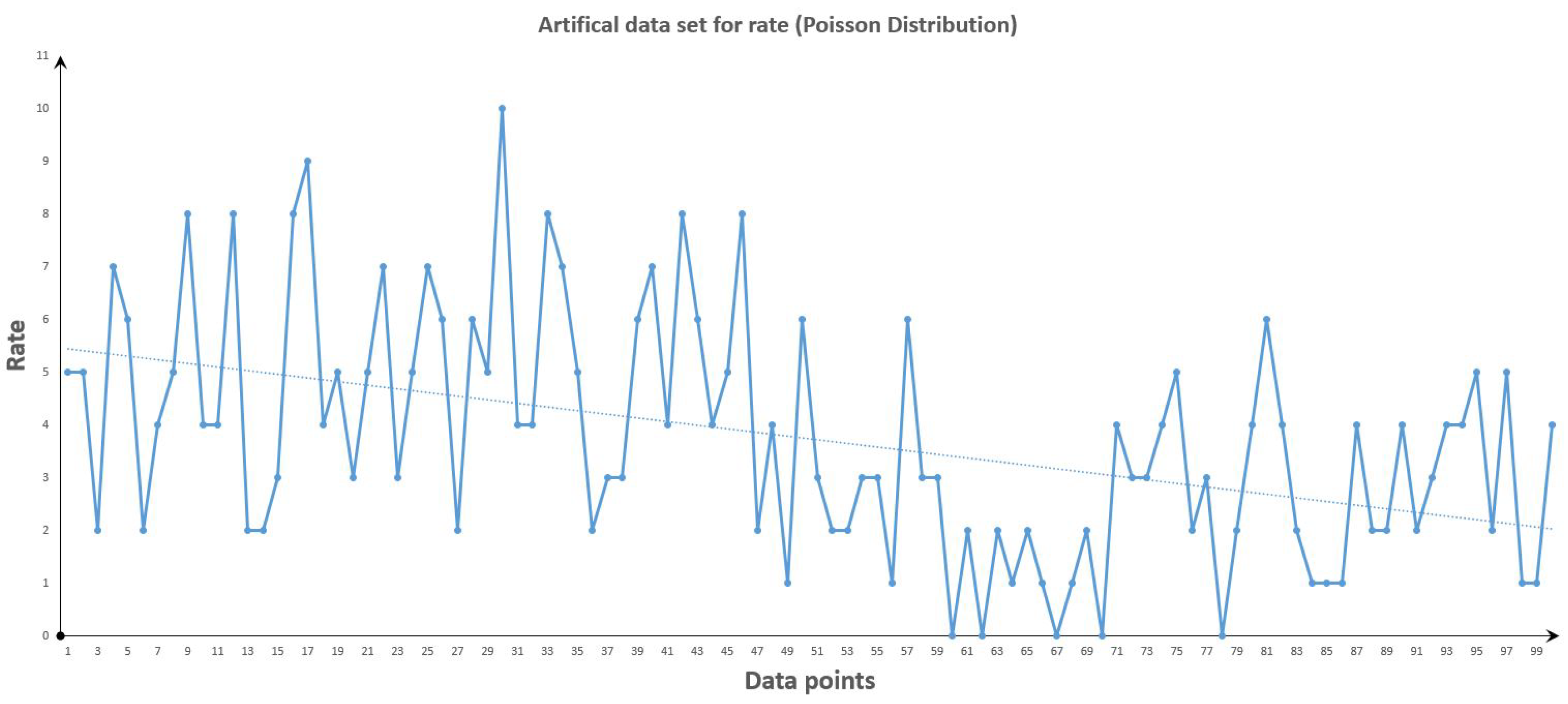
Figure 1.
Artificial Data set for rate (Poisson Distribution).
Figure 1.
Artificial Data set for rate (Poisson Distribution).
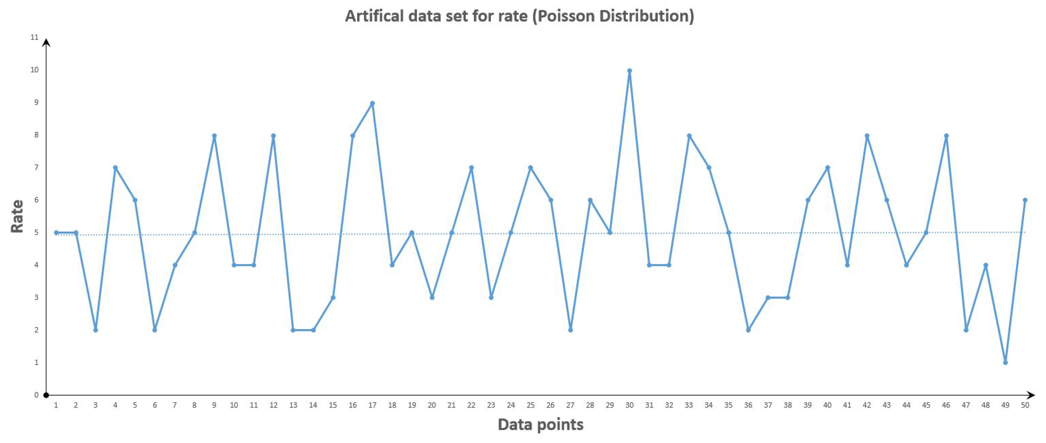
Figure 2.
Artificial Data set for Poisson Distribution before change point.
Figure 2.
Artificial Data set for Poisson Distribution before change point.
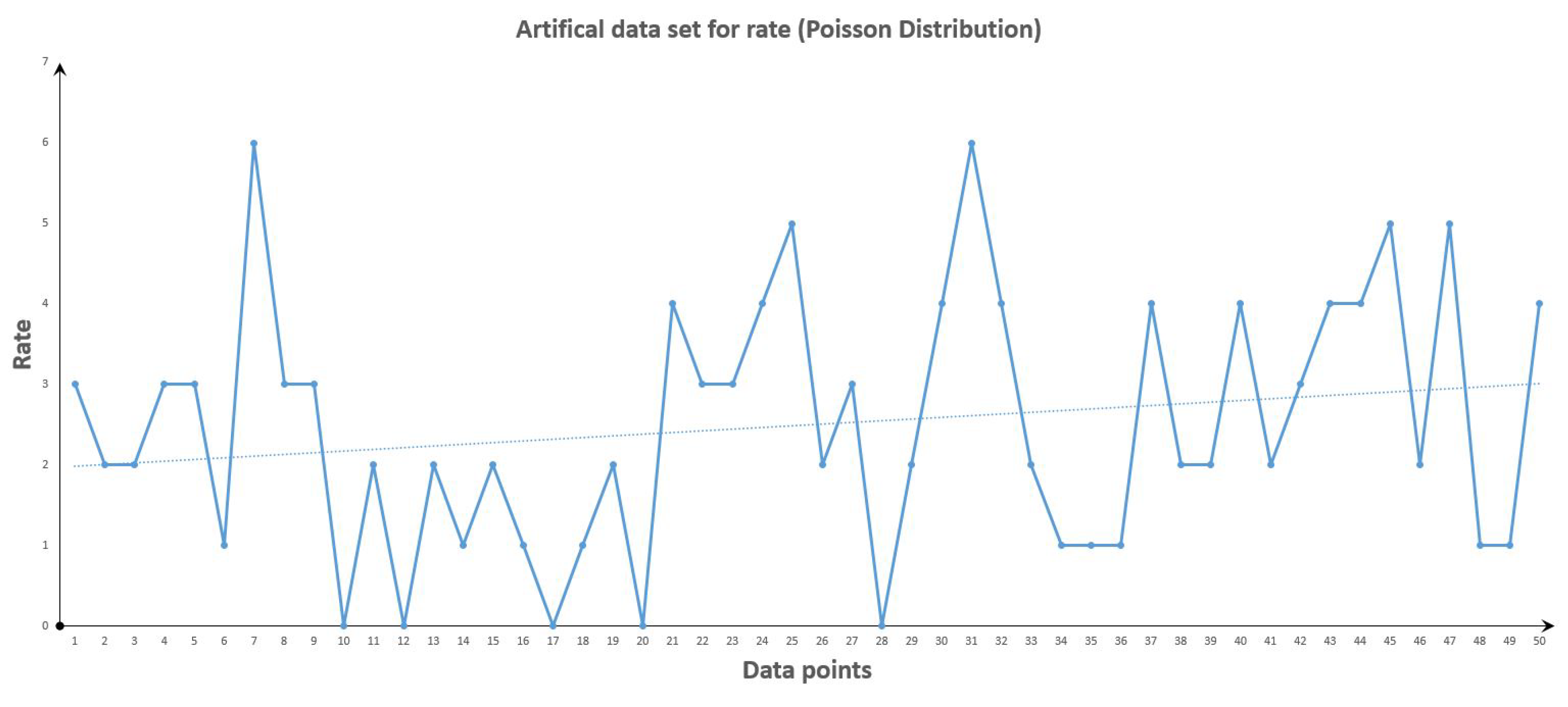
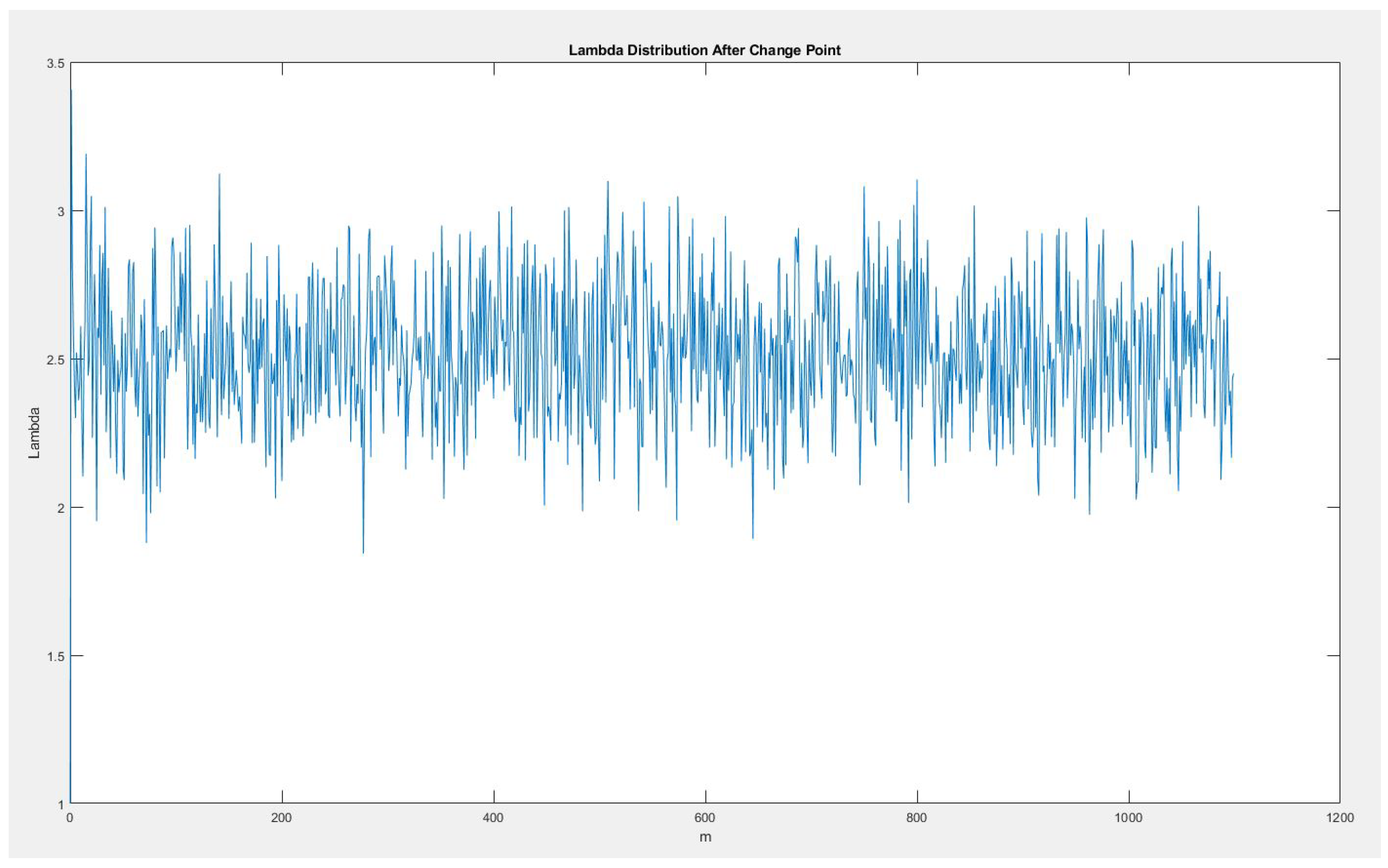
Figure 3.
Artificial Data set for Poisson Distribution after change point.
Figure 3.
Artificial Data set for Poisson Distribution after change point.
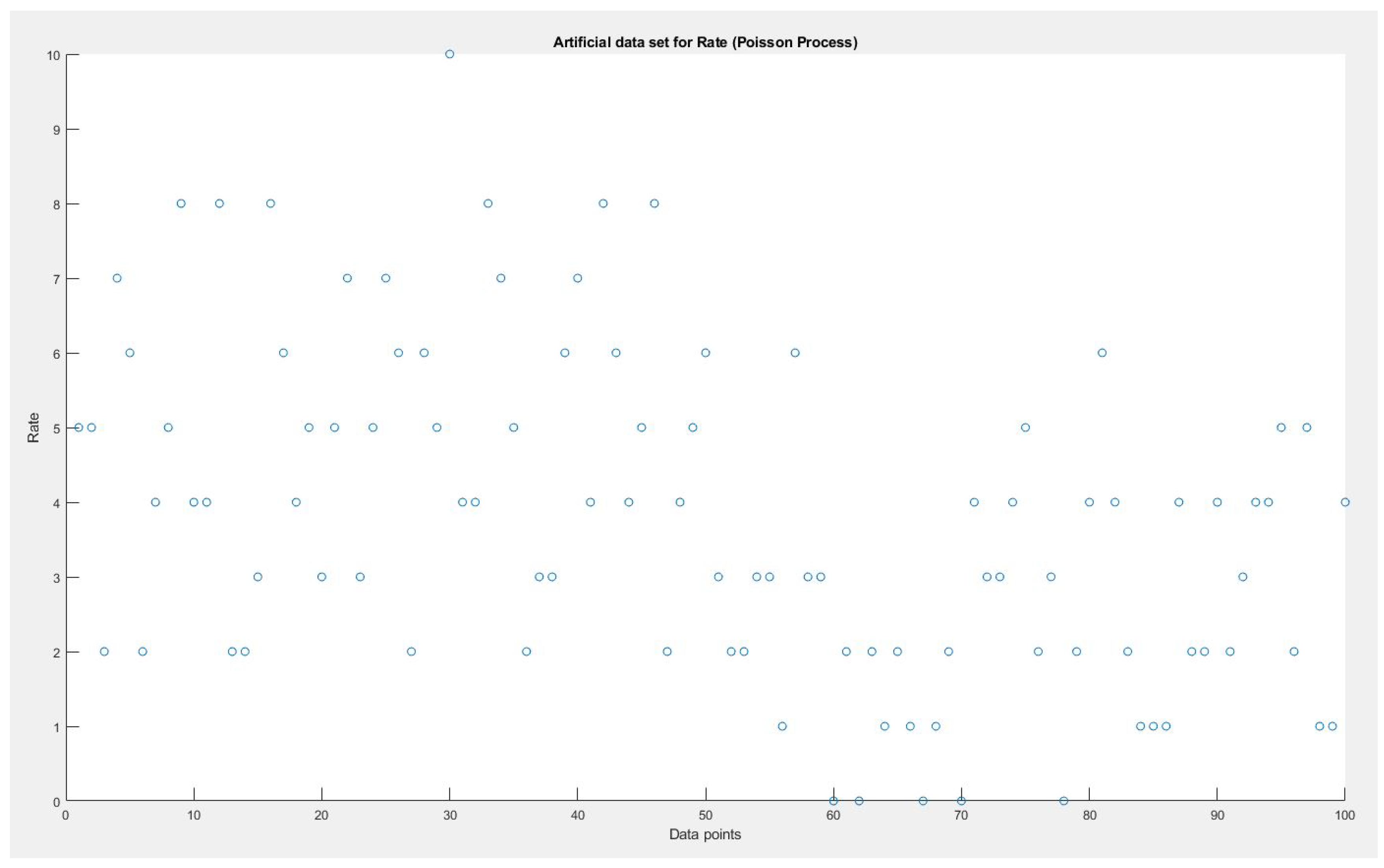
Figure 4.
Artificial Data set time series for Poisson Distribution.
Figure 4.
Artificial Data set time series for Poisson Distribution.
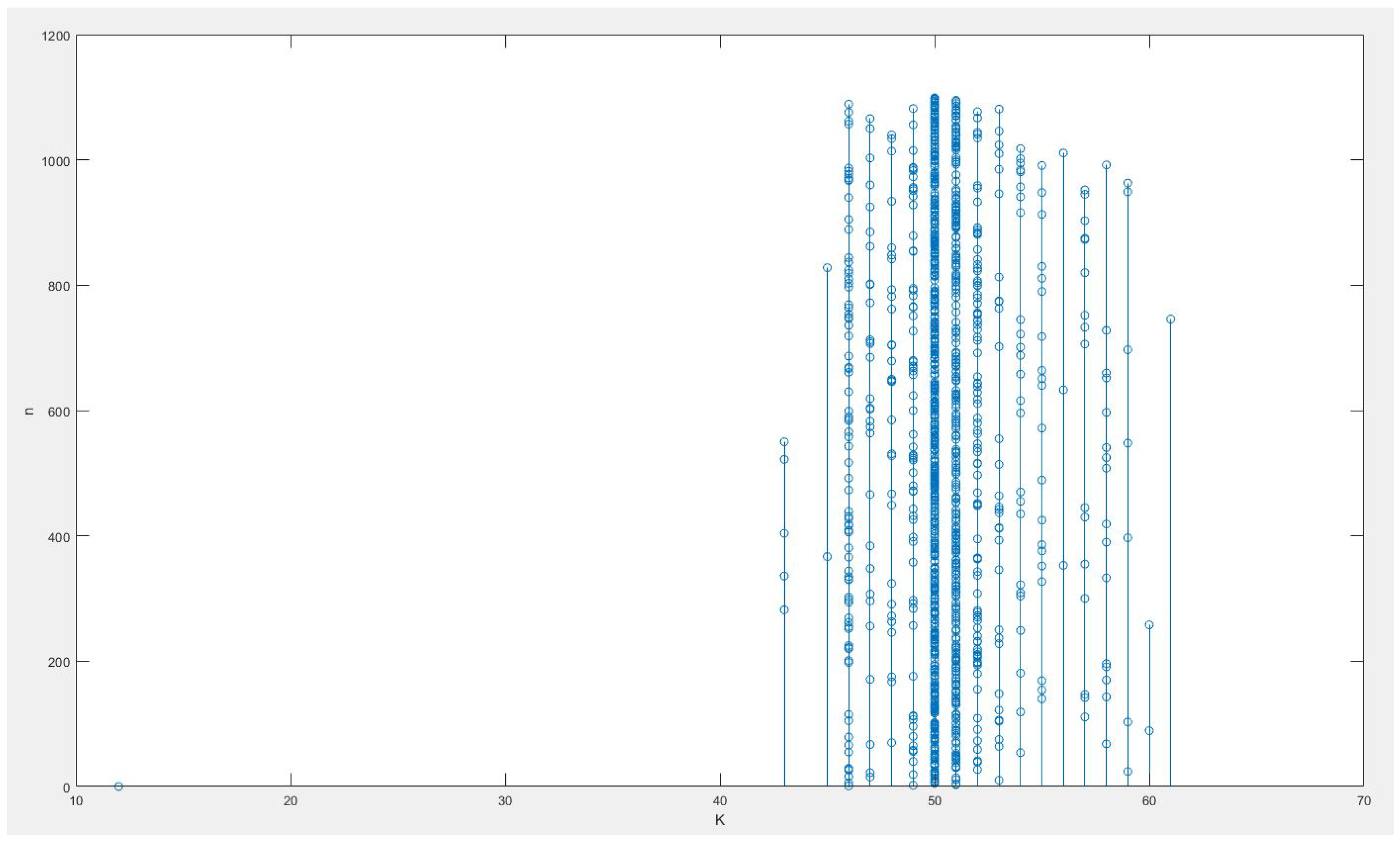
Figure 5.
Change point .
Figure 5.
Change point .
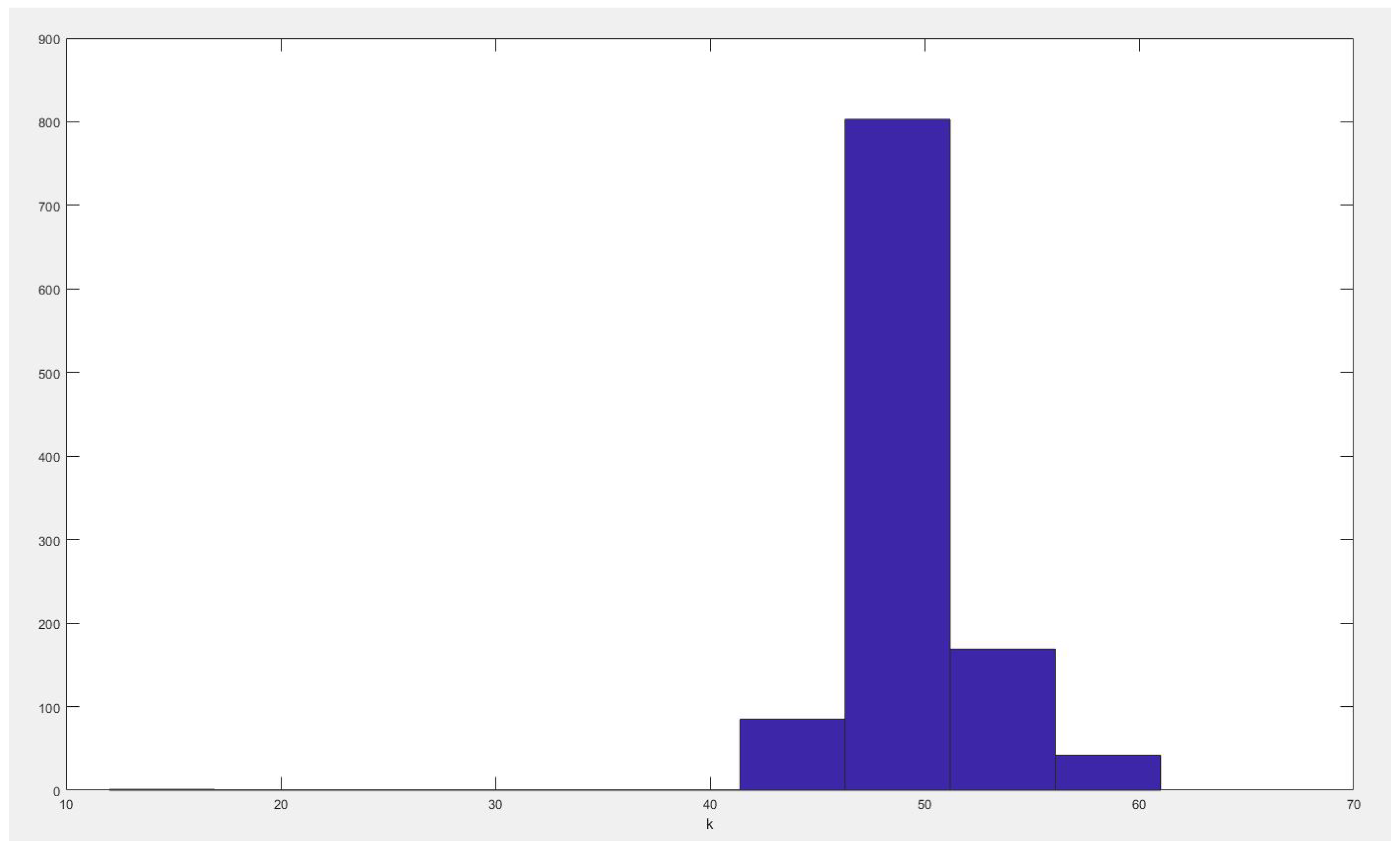
Figure 6.
Change point frequency histogram.
Figure 6.
Change point frequency histogram.
Figure 7.
Change point density histogram.
Figure 7.
Change point density histogram.
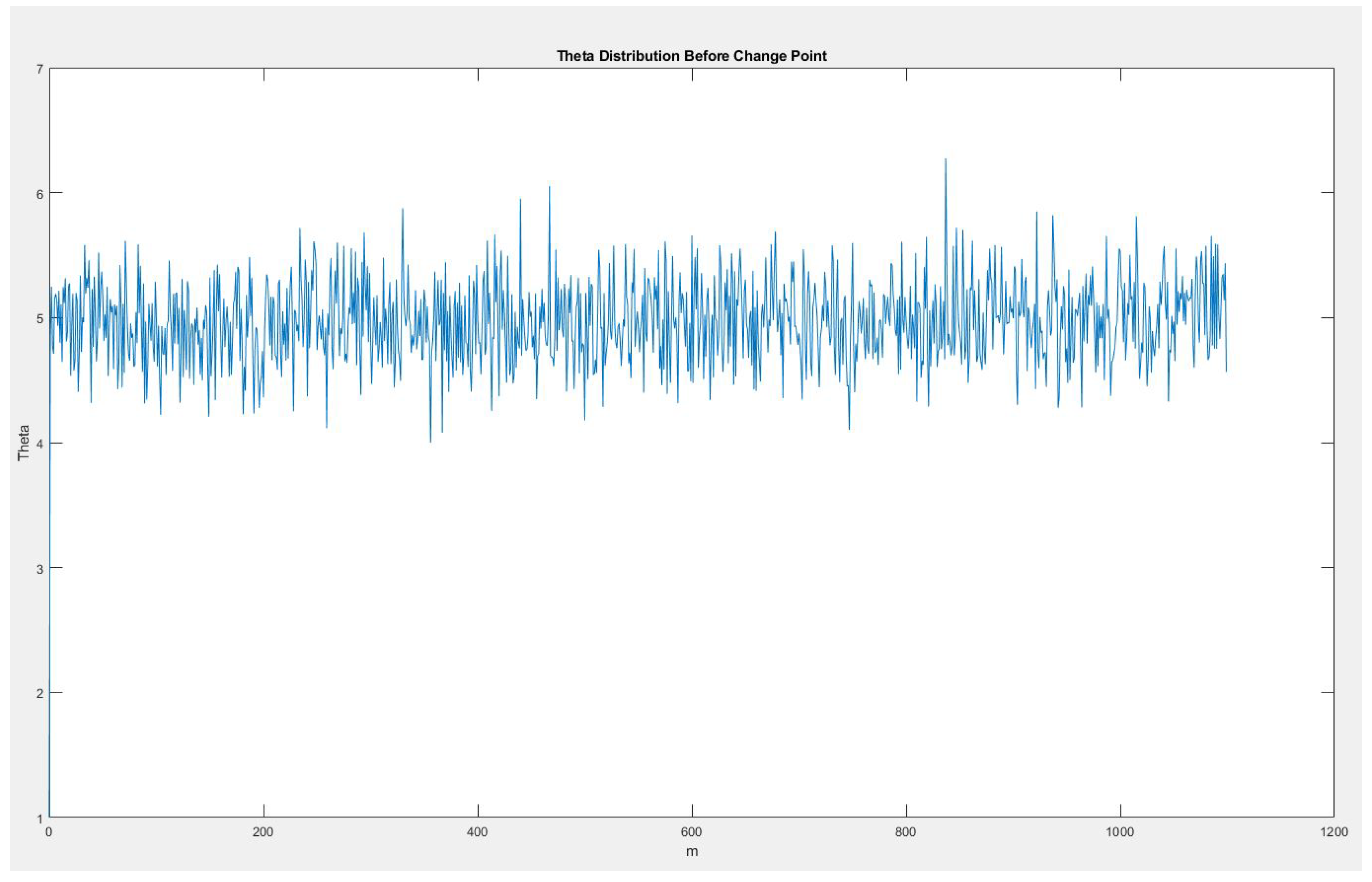
Figure 8.
Rate before change point.
Figure 8.
Rate before change point.
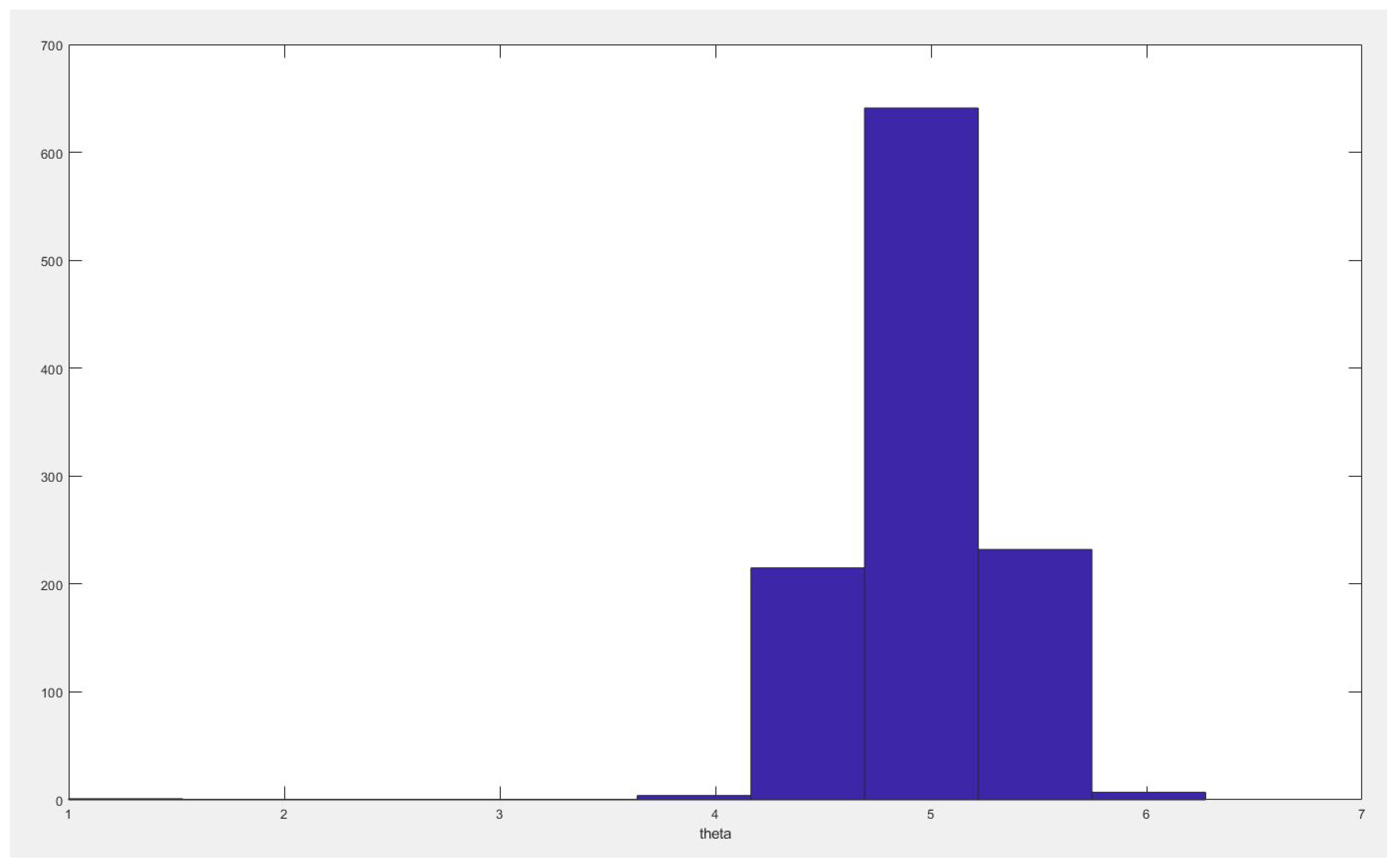
Figure 9.
Rate before change point density histogram.
Figure 9.
Rate before change point density histogram.
Figure 10.
Rate after change point.
Figure 10.
Rate after change point.
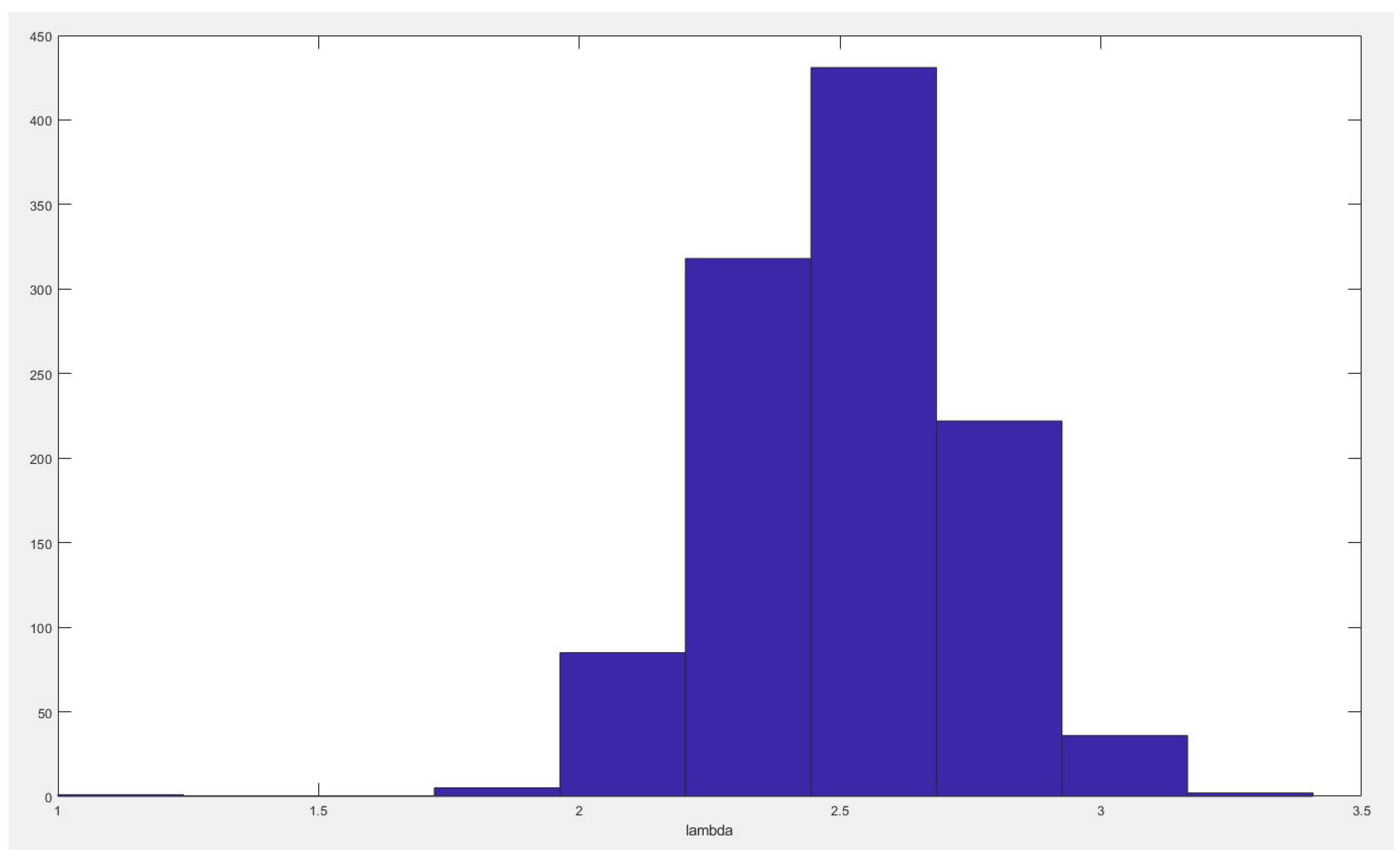
Figure 11.
Rate after change point density histogram.
Figure 11.
Rate after change point density histogram.
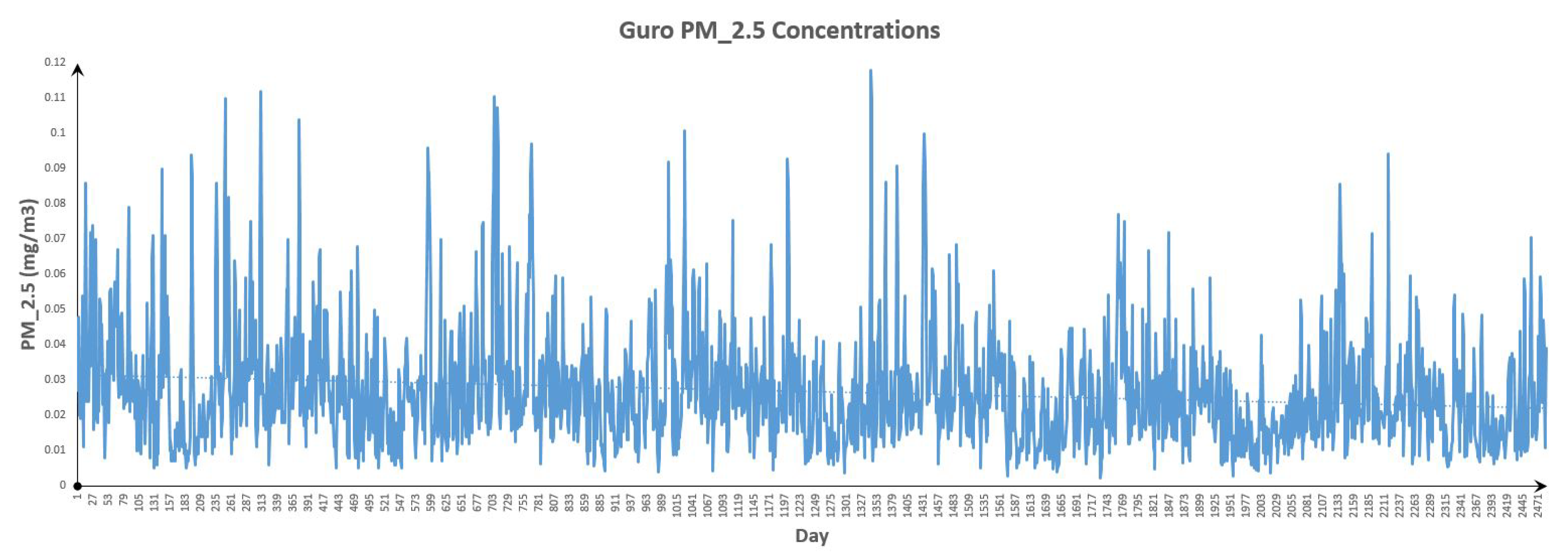
Figure 12.
Guro Data.
Figure 12.
Guro Data.
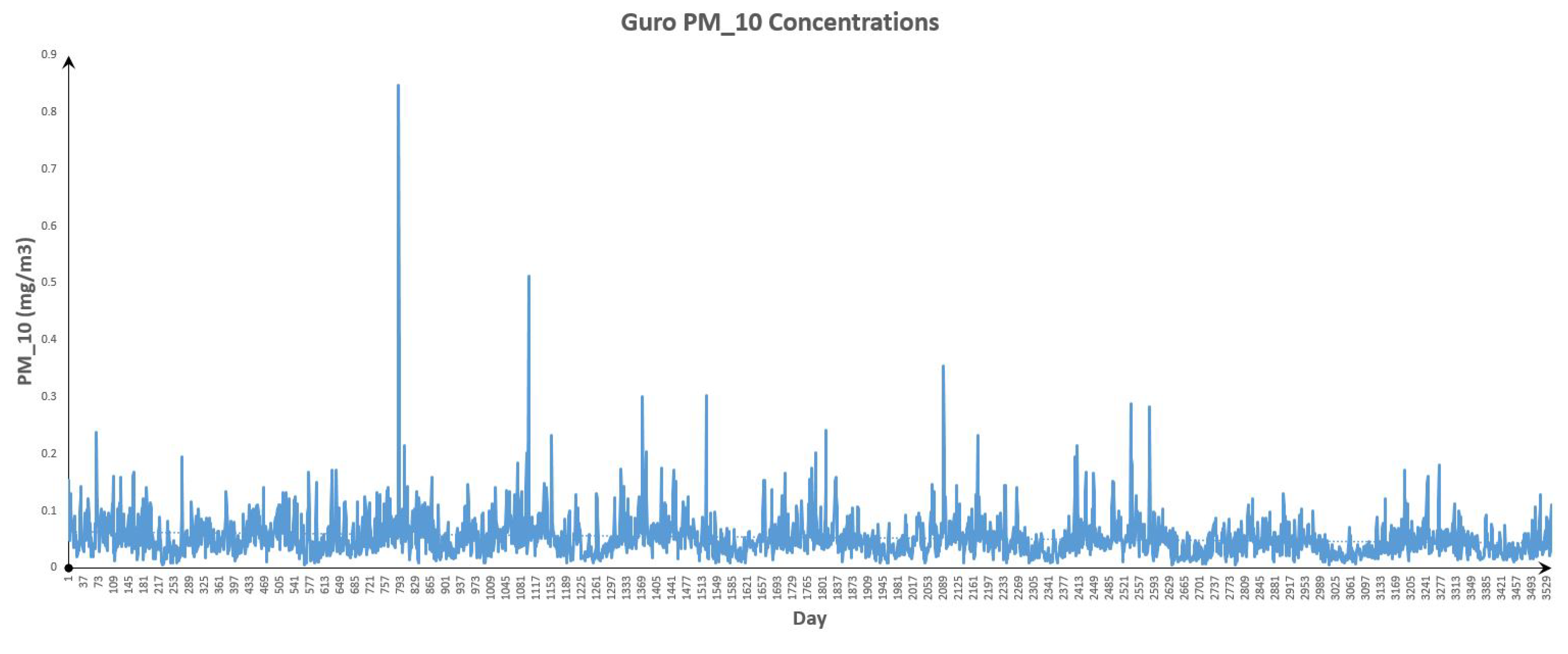
Figure 13.
Guro Data.
Figure 13.
Guro Data.
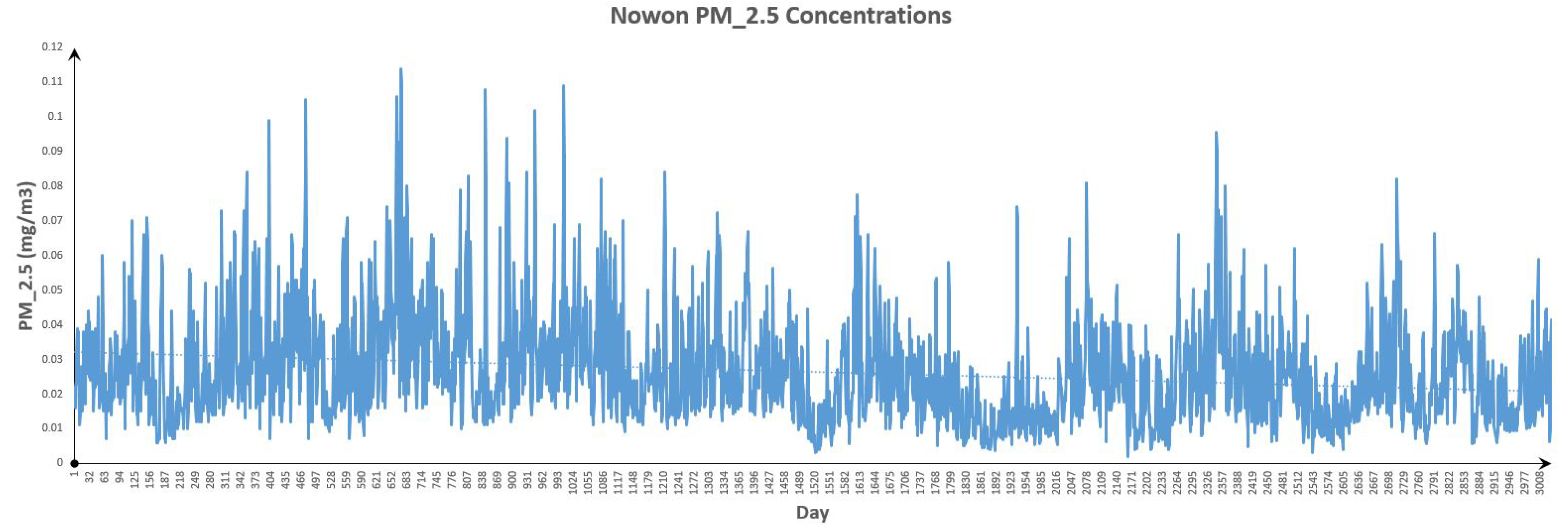
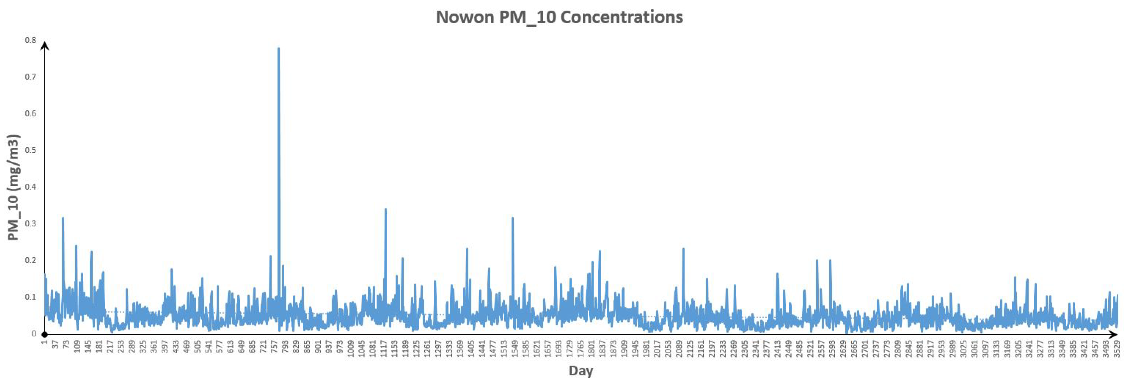
Figure 14.
Nowon Data.
Figure 14.
Nowon Data.
Figure 15.
Nowon Data.
Figure 15.
Nowon Data.
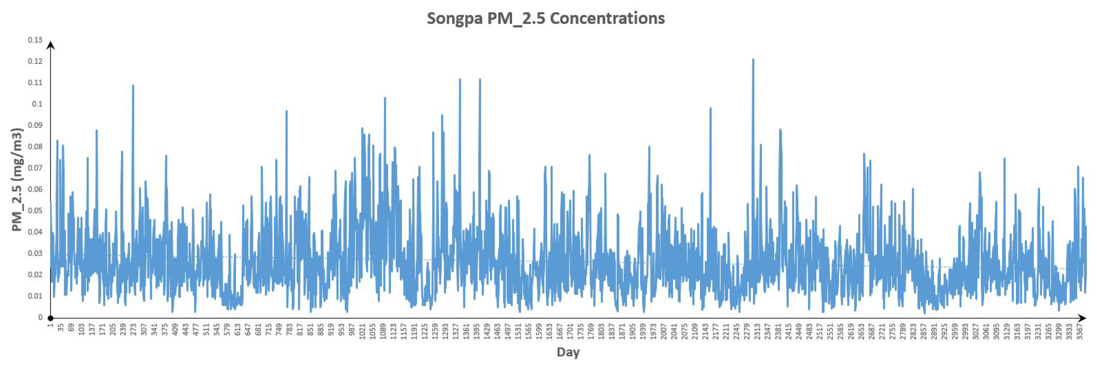
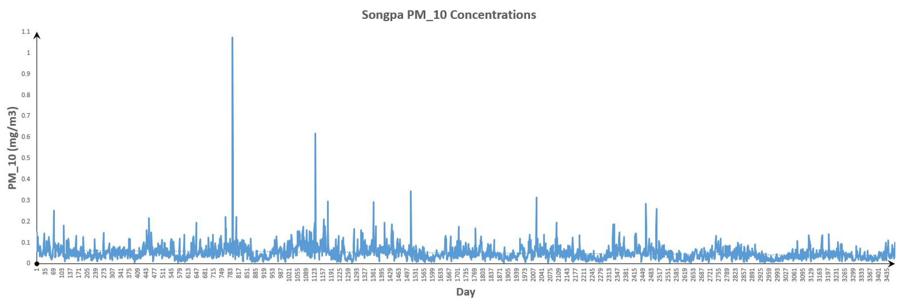
Figure 16.
Songpa Data.
Figure 16.
Songpa Data.
Figure 17.
Songpa Data.
Figure 17.
Songpa Data.
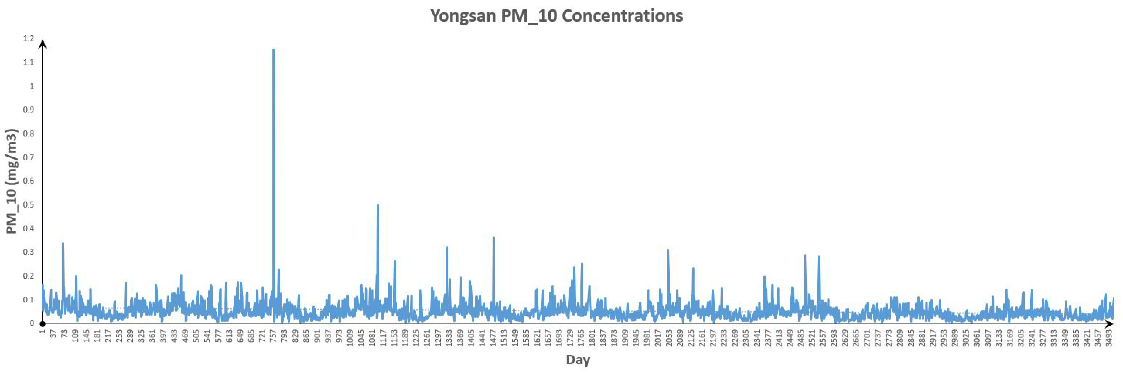
Figure 18.
Yongsan Data.
Figure 18.
Yongsan Data.
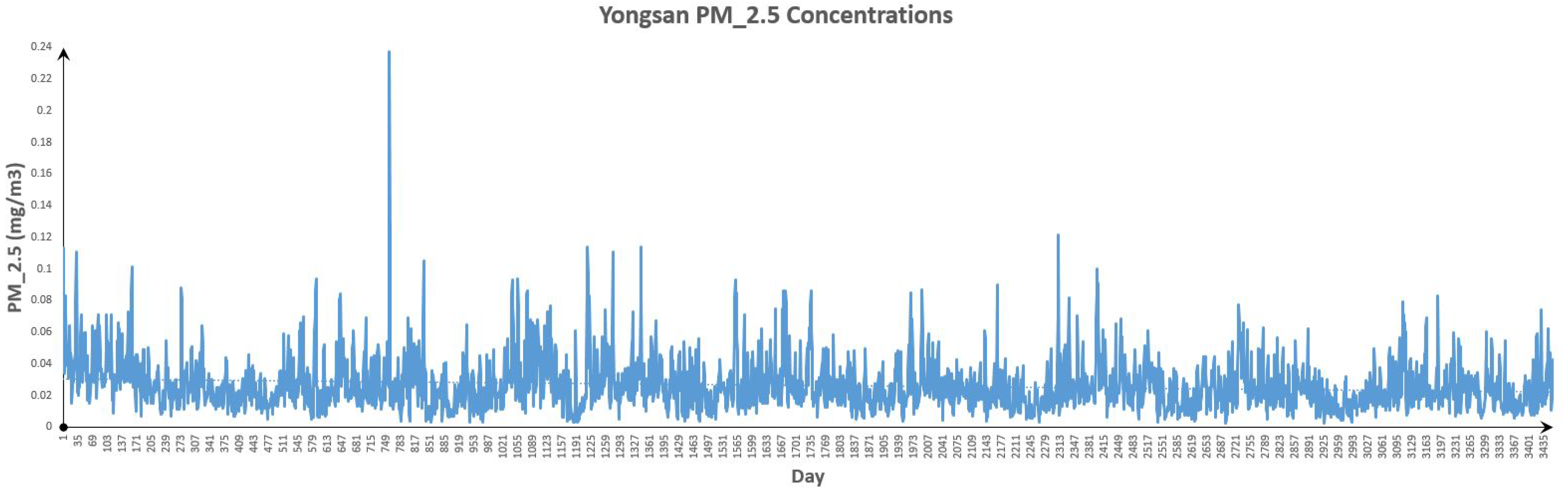
Figure 19.
Yongsan Data.
Figure 19.
Yongsan Data.
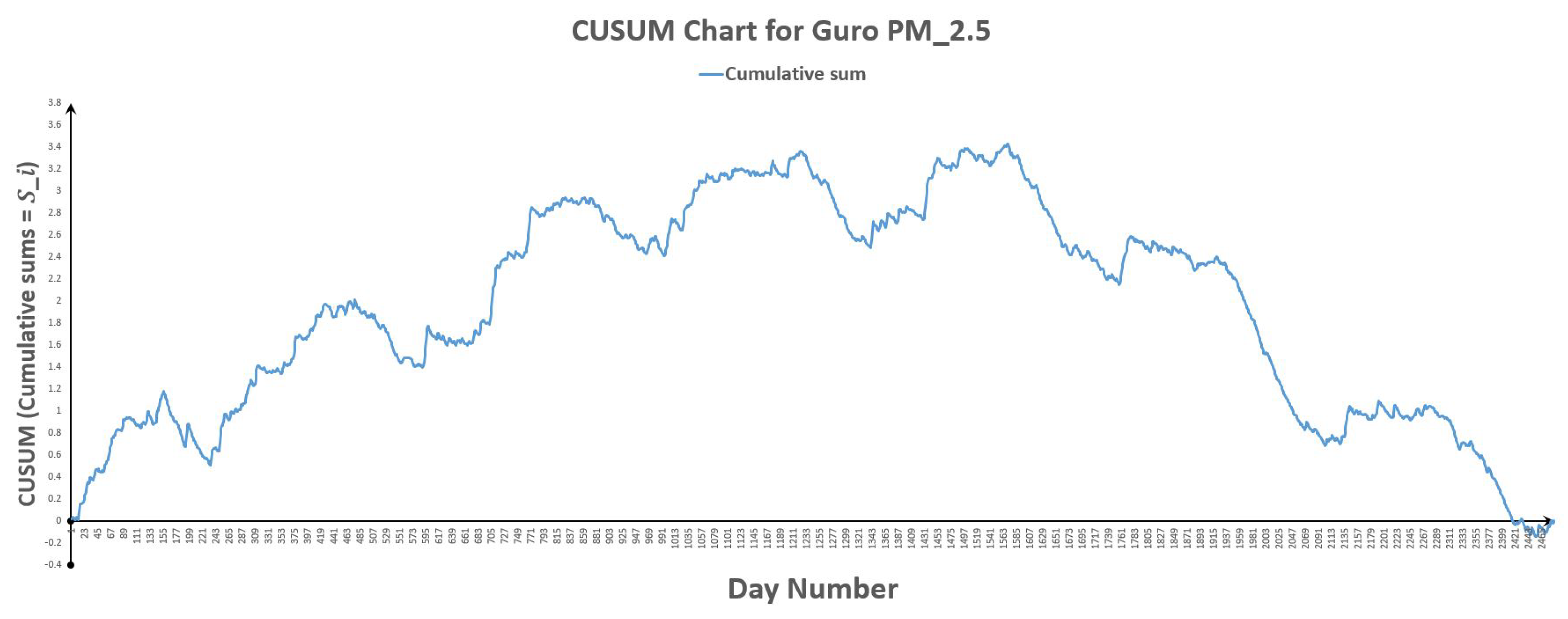
Figure 20.
CUSUM chart for Guro .
Figure 20.
CUSUM chart for Guro .
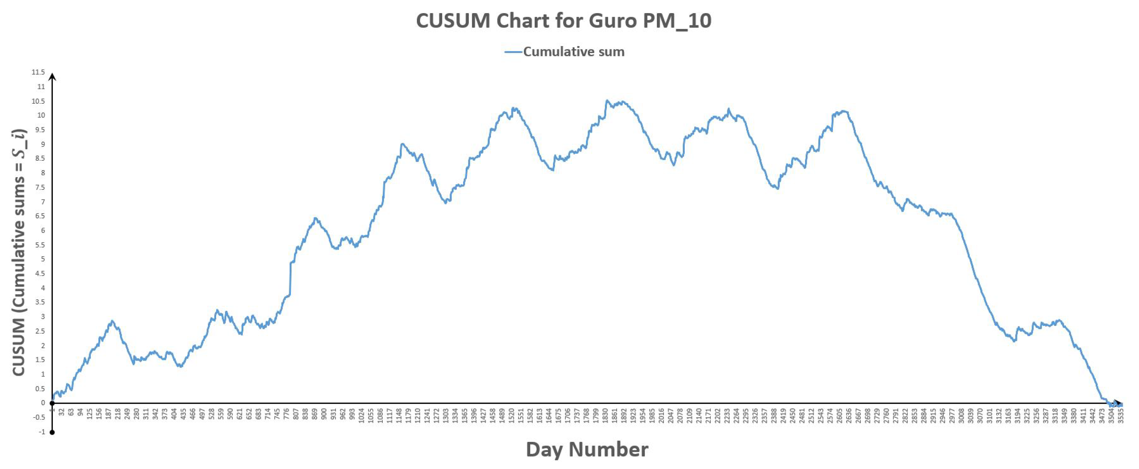
Figure 21.
CUSUM chart for Guro .
Figure 21.
CUSUM chart for Guro .
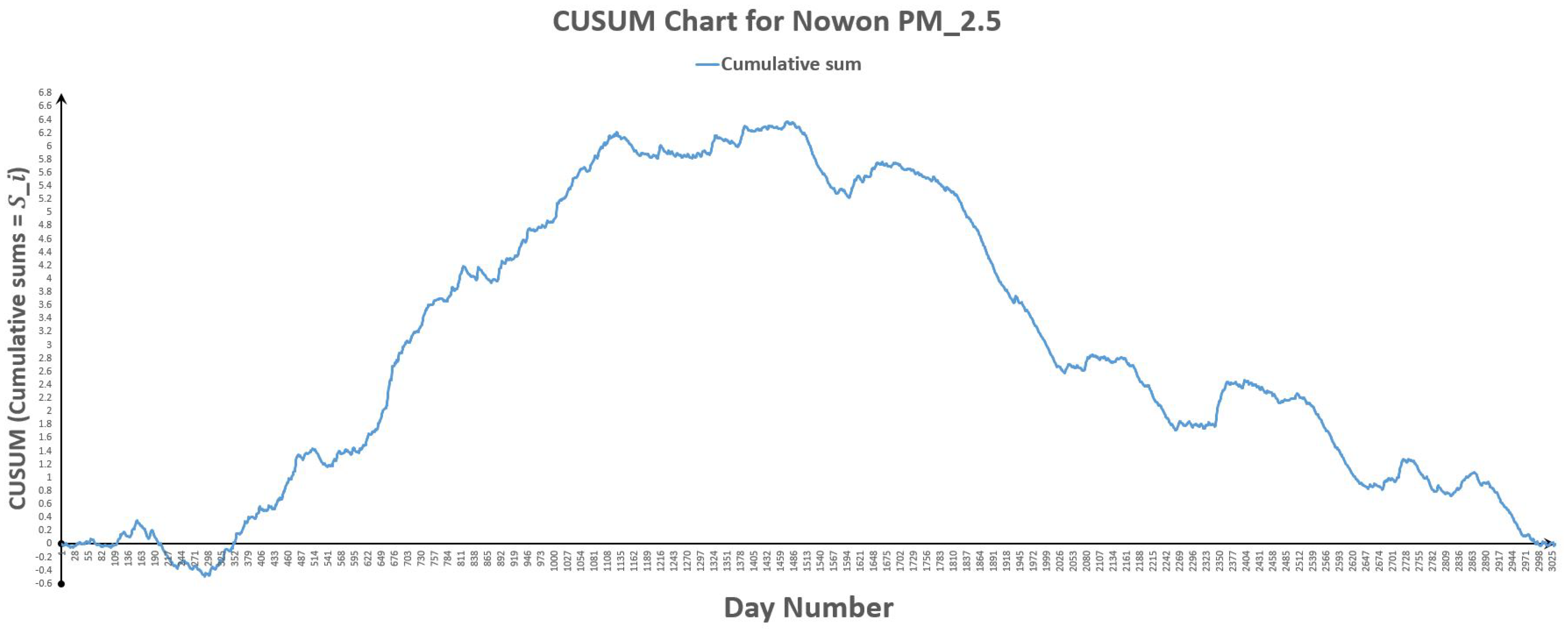
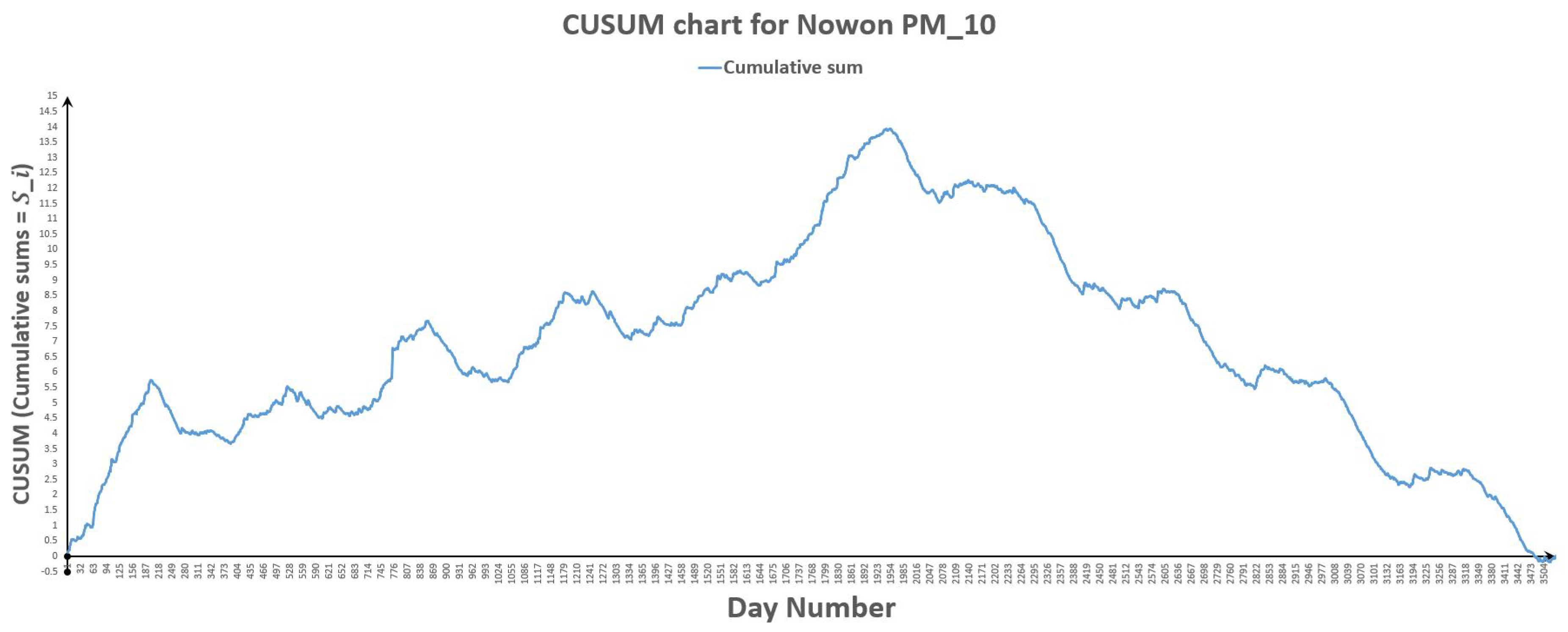
Figure 22.
CUSUM chart for Nowon .
Figure 22.
CUSUM chart for Nowon .
Figure 23.
CUSUM chart for Nowon .
Figure 23.
CUSUM chart for Nowon .
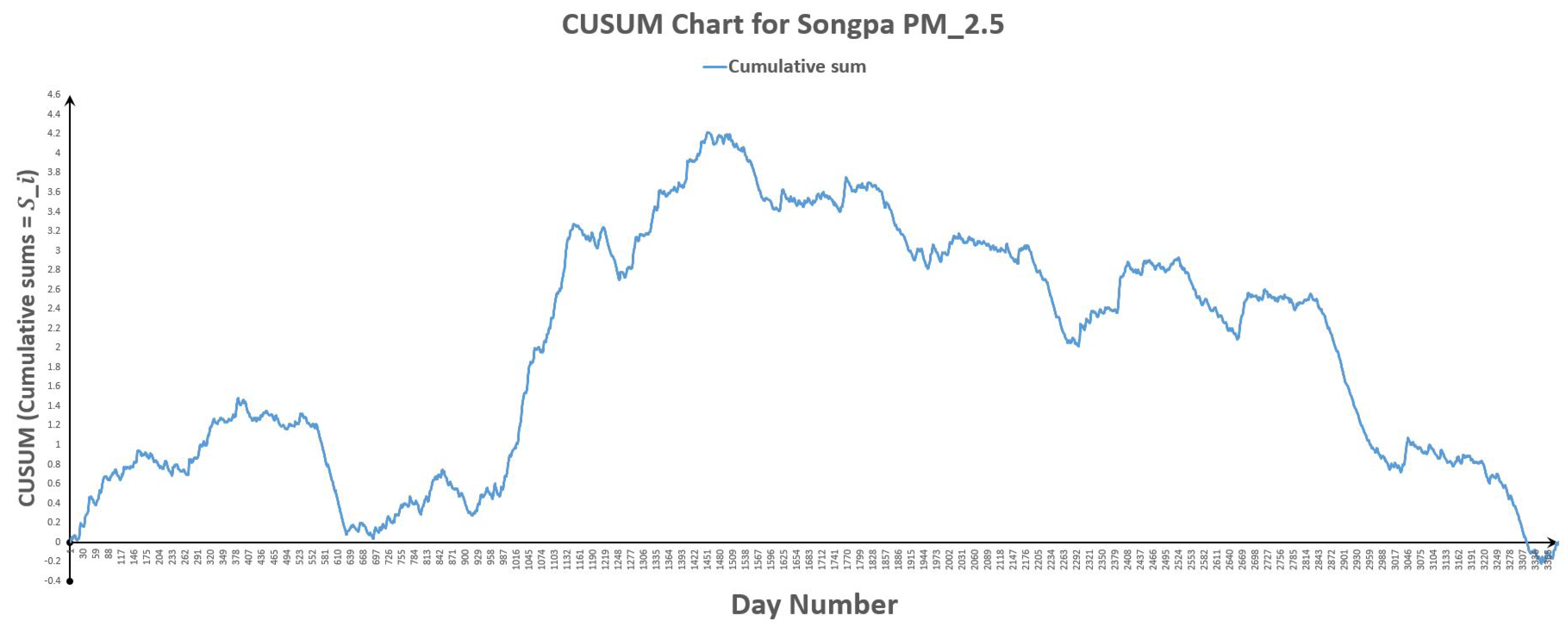
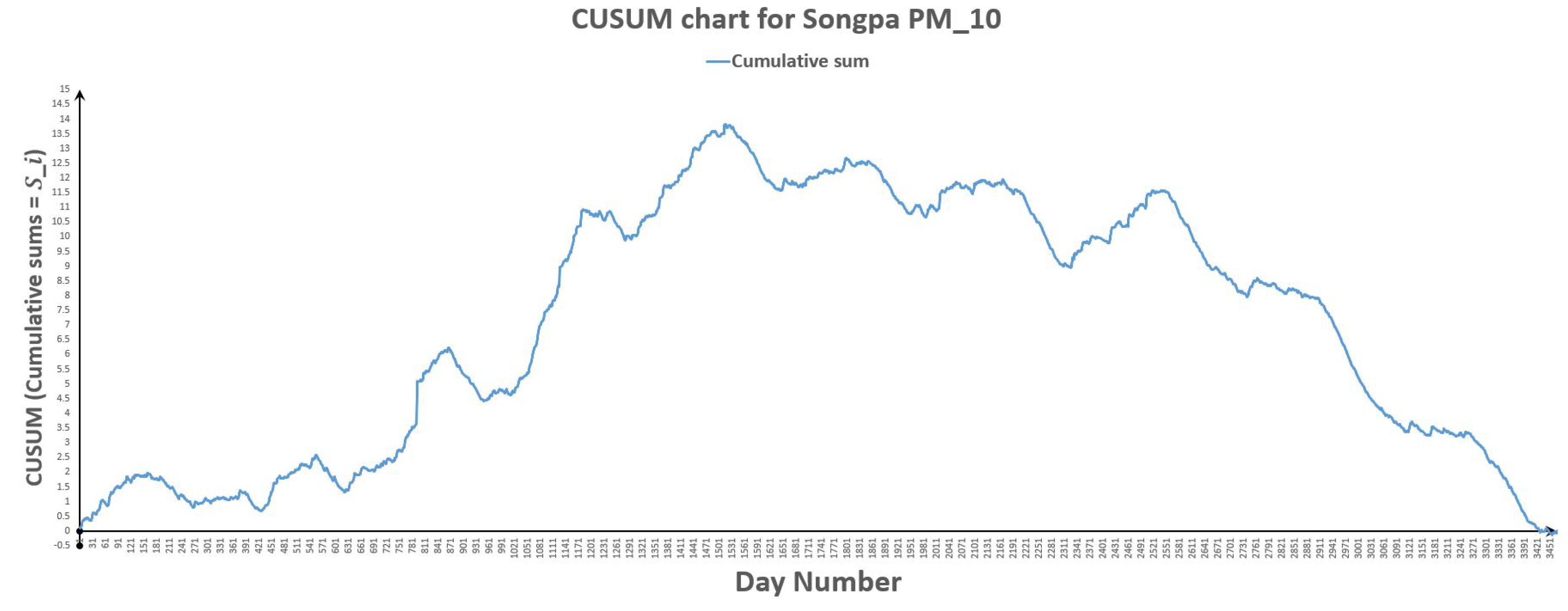
Figure 24.
CUSUM chart for Songpa .
Figure 24.
CUSUM chart for Songpa .
Figure 25.
CUSUM chart for Songpa .
Figure 25.
CUSUM chart for Songpa .
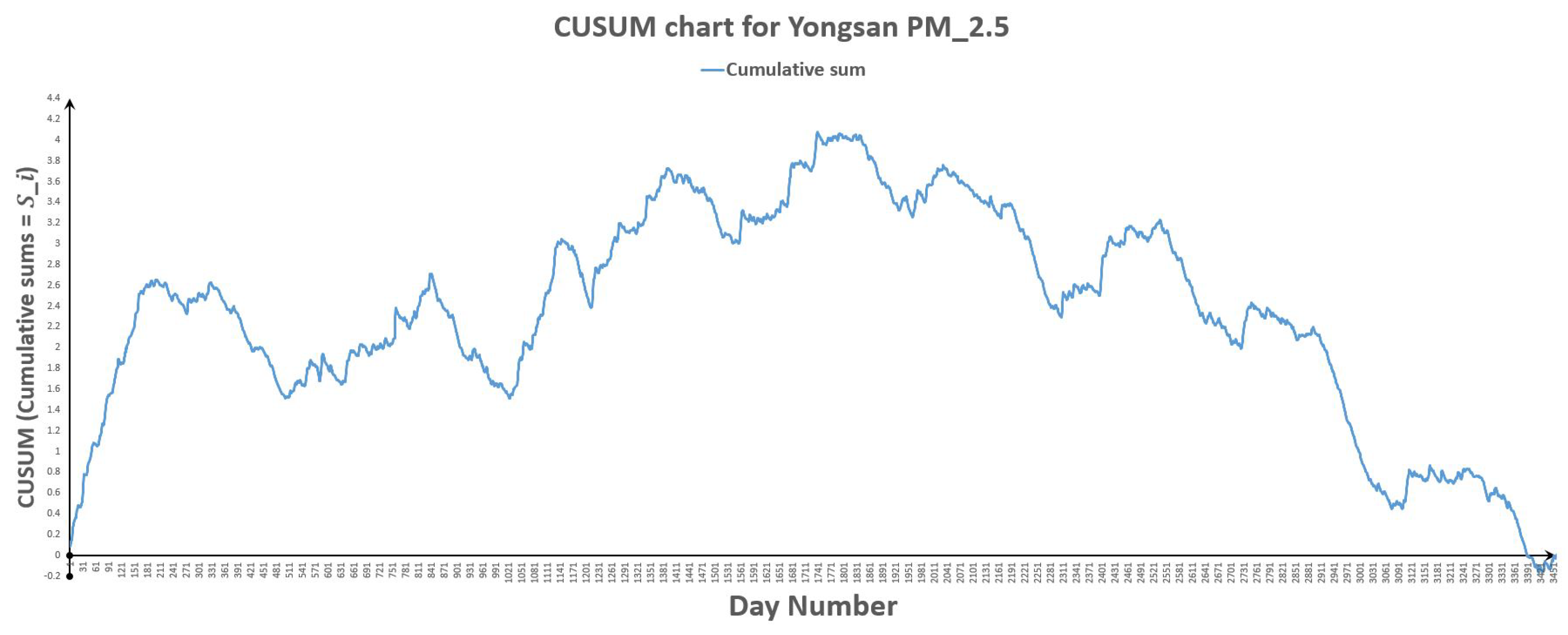
Figure 26.
CUSUM chart for Yongsan .
Figure 26.
CUSUM chart for Yongsan .
Figure 27.
CUSUM chart for Yongsan .
Figure 27.
CUSUM chart for Yongsan .
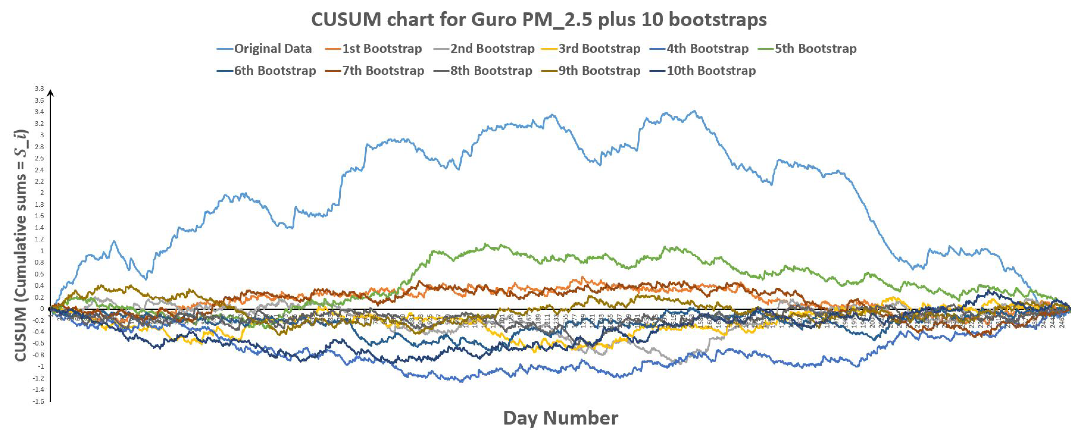
Figure 28.
CUSUM chart for Guro plus 10 bootstraps.
Figure 28.
CUSUM chart for Guro plus 10 bootstraps.
Figure 29.
CUSUM chart for Guro plus 10 bootstraps.
Figure 29.
CUSUM chart for Guro plus 10 bootstraps.
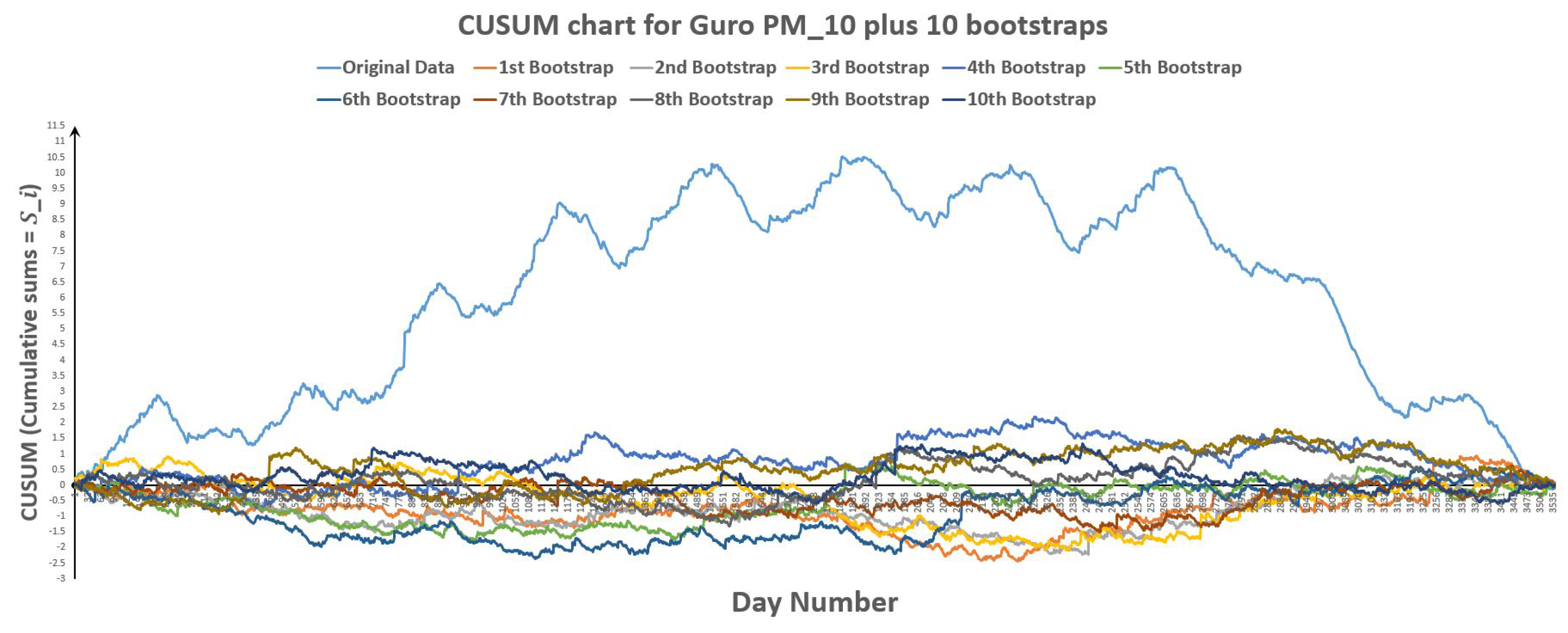
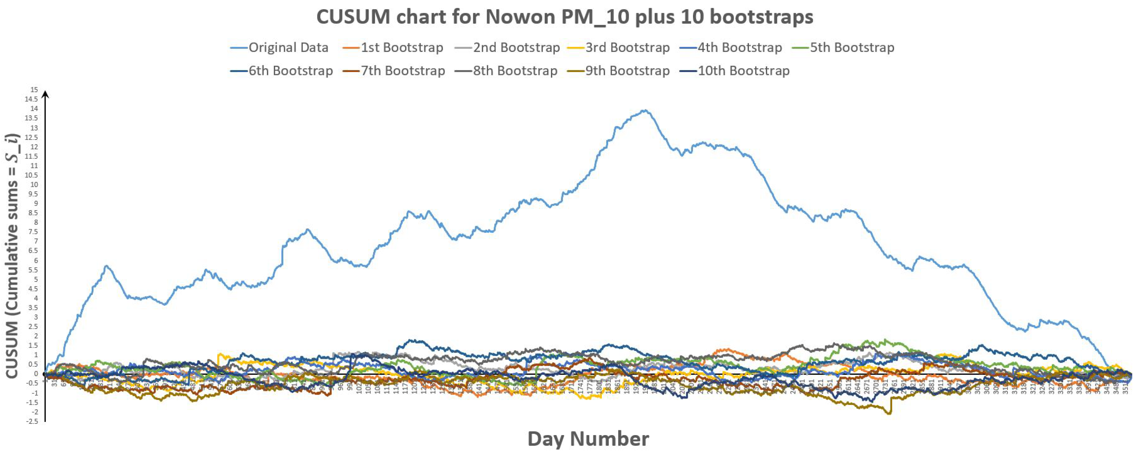
Figure 30.
CUSUM chart for Nowon plus 10 bootstraps.
Figure 30.
CUSUM chart for Nowon plus 10 bootstraps.
Figure 31.
CUSUM chart for Nowon plus 10 bootstraps.
Figure 31.
CUSUM chart for Nowon plus 10 bootstraps.
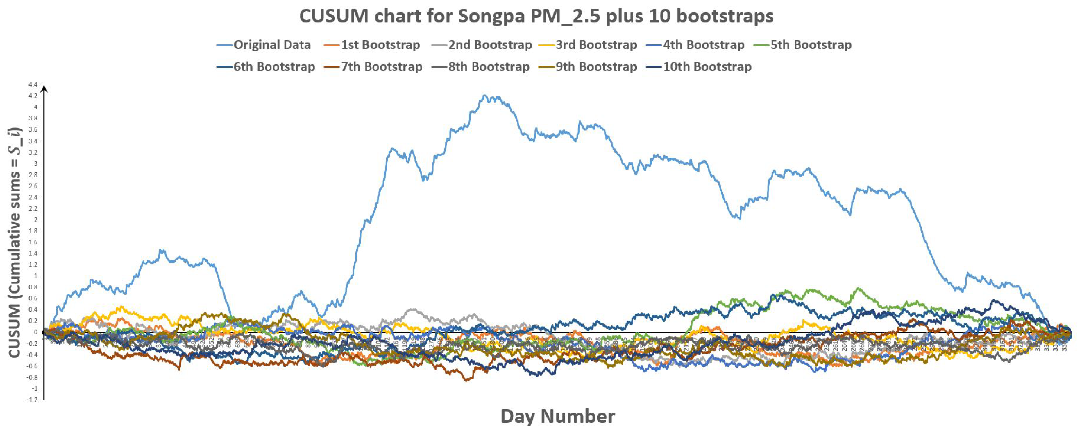
Figure 32.
CUSUM chart for Songpa plus 10 bootstraps.
Figure 32.
CUSUM chart for Songpa plus 10 bootstraps.
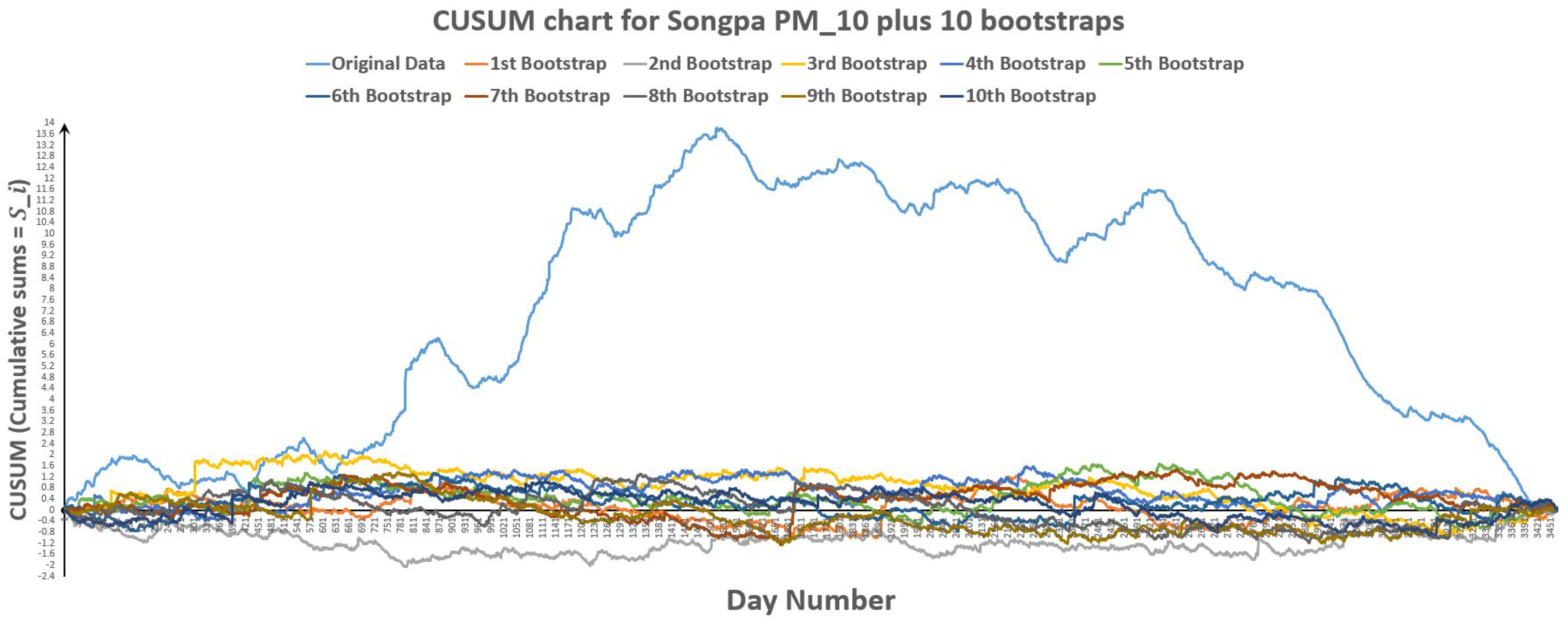
Figure 33.
CUSUM chart for Songpa plus 10 bootstraps.
Figure 33.
CUSUM chart for Songpa plus 10 bootstraps.
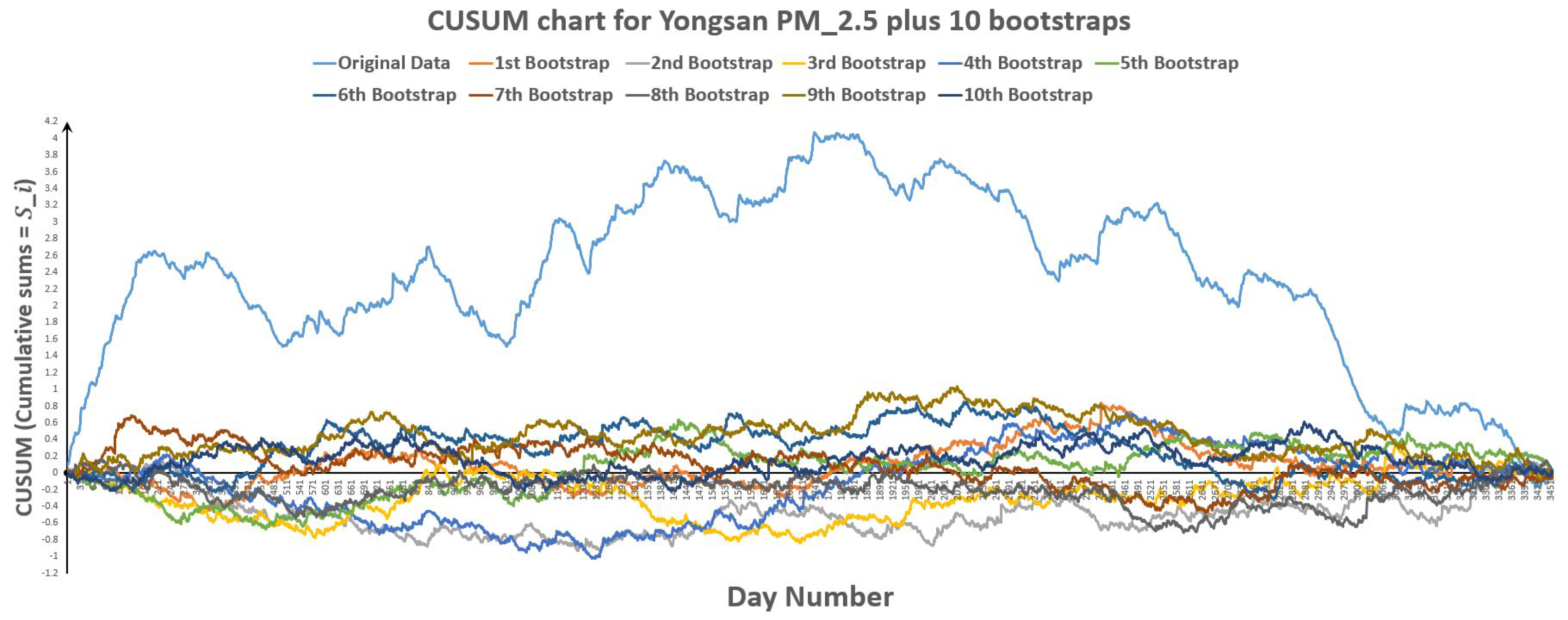
Figure 34.
CUSUM chart for Yongsan plus 10 bootstraps.
Figure 34.
CUSUM chart for Yongsan plus 10 bootstraps.
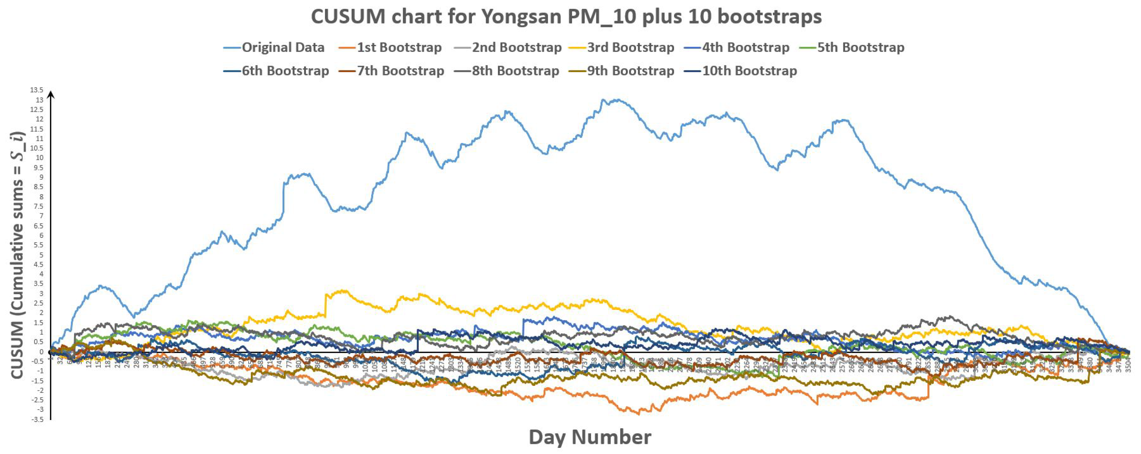
Figure 35.
CUSUM chart for Yongsan plus 10 bootstraps.
Figure 35.
CUSUM chart for Yongsan plus 10 bootstraps.
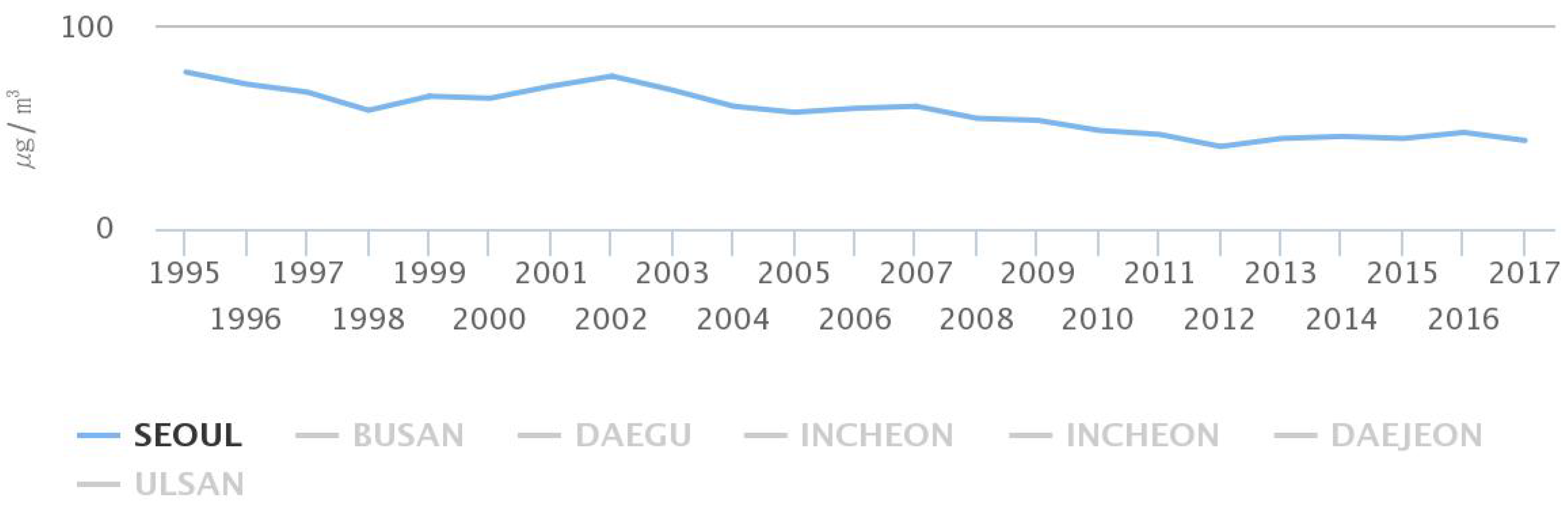
Figure 36.
Annual Particulate Matter trend in Seoul (airkorea).
Figure 36.
Annual Particulate Matter trend in Seoul (airkorea).
Table 1.
Previous studies on this topic.
Table 1.
Previous studies on this topic.
| Document | Change-Point Detection | BCPD | Time Series |
|---|
| (Bayesian Change-Point Detection) |
|---|
| Cabrieto et al. (2018) [4] | Kernel change point detection, | - | - |
| | correlation changes | - | - |
| Keshavarz et al. (2018) [5] | Generalized likelihood ratio test, | - | - |
| | One-dimensional Gaussian process | - | - |
| Kucharczyk et al. (2018) [6] | Likelihood ratio test, | - | - |
| | fractional Brownian motion | - | - |
| Lu et al. (2017) [8] | Change-point detection, machine monitoring, | - | Time Series |
| | Anomaly measure (AR model), Martingale test | - | |
| | On-line change detection, | - | - |
| Hilgert et al. (2016) [11] | autoregressive dynamic models, | - | - |
| | CUSUM-like scheme | - | - |
| Górecki et al. (2017) [13] | Change point detection, heteroscedastic, | - | Time series |
| | Karhunen-Loeve expansions | - | |
| Bucchia and Wendler (2017) [14] | Change point detection, bootstrap, | - | |
| | Hilbert space valued random fields, | - | Time series |
| | (Cramer–von Mises type test) | - | |
| Zhou et al. (2015) [16] | Sequential change point detection, | - | - |
| | linear quantile regression models | - | - |
| Lu and Chang (2016) [18] | Detecting change points, | - | - |
| | mean/variance shifts, FCML-CP algorithm | - | - |
| Liu et al. (2013) [10] | Change point detection, | - | Time series |
| | relative density ratio estimation | - | |
| Ruggieri and Antonellis (2016) [19] | - | Bayesian sequential change point detection | - |
| Keshavarz and Huang (2014) [25] | - | Bayesian and Expectation Maximization methods, | - |
| | - | multivariate change point detection | - |
| Kurt et al. (2018) [27] | - | Bayesian change point model, | - |
| | - | SIP-based DDoS attacks detection | - |
| Wu et al. (2017) [28] | - | Post classification change detection, | - |
| | - | iterative slow feature analysis, | - |
| | - | Bayesian soft fusion | - |
| Gupta and Baker (2017) [22] | - | Spatial event rates, change point, | - |
| | - | Bayesian statistics, induced seismicity | - |
| Marino et al. (2017) [30] | - | Change point, multiple biomarkers, | - |
| | - | ovarian cancer | - |
| Jeon et al. (2016) [32] | - | Abrupt change point detection, | - |
| | - | annual maximum precipitation, fused lasso | - |
| Bardwell and Fearnhead (2017) [23] | - | Bayesian Detection, Abnormal Segments | Time series |
| Chen et al. (2017) [34] | - | Bayesian change point analysis, | - |
| | - | extreme daily precipitation | - |
| | | Bayesian approach and | |
| This study | Change point detection | likelihood ratio test for | Time series |
| | | change point detection | |
Table 2.
Change point (k) for artificial data set.
Table 2.
Change point (k) for artificial data set.
| Change Point (k) for Artificial Data Set |
|---|
| | K |
| before change | after change | change point |
| 5.0 | 2.5 | 50 |
Table 3.
Normal distribution.
Table 3.
Normal distribution.
| Normal Distribution |
|---|
| Area | | |
| Mean Is the Location | Variance Is Scale or Deviation |
| Guro | 0.02675 | 0.01614 |
| Nowon | 0.02652 | 0.01551 |
| Songpa | 0.02638 | 0.01544 |
| Yongsan | 0.02649 | 0.01621 |
Table 4.
Normal distribution.
Table 4.
Normal distribution.
| Normal Distribution |
|---|
| Area | | |
| | Mean Is the Location | Variance Is Scale or Deviation |
| Guro | 0.05340 | 0.03644 |
| Nowon | 0.05036 | 0.03331 |
| Songpa | 0.05193 | 0.03811 |
| Yongsan | 0.05379 | 0.03958 |
Table 5.
Converged values of parameters (Probabilistic Method)
Table 5.
Converged values of parameters (Probabilistic Method)
| Converged Values of Parameters (Probabilistic Method) |
|---|
| | Guro | Nowon |
| Replication | | | | | K | | | | | K |
| mean | Replication | Replication | Replication | Replication | Replication | Replication | Replication | Replication | Replication | Replication |
| | mean | mean | mean | mean | mean | mean | mean | mean | mean | mean |
| 0.0293 | 0.0246 | | | 1229.02 | 0.0296 | 0.0235 | | | 1497.30 |
| 0.0292 | 0.0246 | | | 1261.72 | 0.0296 | 0.0235 | | | 1529.49 |
| 0.0294 | 0.0246 | | | 1199.08 | 0.0296 | 0.0236 | | | 1475.20 |
| 0.0294 | 0.0246 | | | 1214.48 | 0.0295 | 0.0236 | | | 1485.39 |
| 0.0292 | 0.0246 | | | 1232.26 | 0.0295 | 0.0235 | | | 1527.50 |
| 0.0294 | 0.0246 | | | 1202.37 | 0.0295 | 0.0236 | | | 1478.39 |
| 0.0293 | 0.0247 | | | 1236.93 | 0.0294 | 0.0236 | | | 1497.28 |
| 0.0292 | 0.0246 | | | 1248.80 | 0.0295 | 0.0235 | | | 1524.84 |
| 0.0293 | 0.0245 | | | 1253.42 | 0.0295 | 0.0235 | | | 1525.16 |
| 0.0294 | 0.0247 | | | 1206.30 | 0.0294 | 0.0236 | | | 1487.82 |
| | | | | | | | | | |
| Mean of 10 | 0.0293 | 0.0246 | | | 1228.44 | 0.0295 | 0.0235 | | | 1502.84 |
| replications | | | | | | | | | | |
| | Songpa | Yongsan |
| Replication | | | | | K | | | | | K |
| mean | Replication | Replication | Replication | Replication | Replication | Replication | Replication | Replication | Replication | Replication |
| | mean | mean | mean | mean | mean | mean | mean | mean | mean | mean |
| 0.0280 | 0.0245 | | | 1788.62 | 0.0302 | 0.0248 | | | 1563.53 |
| 0.0281 | 0.0245 | | | 1753.39 | 0.0302 | 0.0248 | | | 1534.23 |
| 0.0282 | 0.0245 | | | 1709.28 | 0.0308 | 0.0249 | | | 1457.41 |
| 0.0281 | 0.0246 | | | 1725.05 | 0.0308 | 0.0249 | | | 1482.48 |
| 0.0281 | 0.0245 | | | 1774.62 | 0.0303 | 0.0249 | | | 1543.11 |
| 0.0282 | 0.0246 | | | 1702.20 | 0.0308 | 0.0249 | | | 1476.89 |
| 0.0282 | 0.0247 | | | 1732.44 | 0.0313 | 0.0249 | | | 1458.11 |
| 0.0280 | 0.0246 | | | 1768.74 | 0.0303 | 0.0248 | | | 1552.81 |
| 0.0281 | 0.0245 | | | 1785.43 | 0.0304 | 0.0248 | | | 1545.42 |
| 0.0282 | 0.0245 | | | 1718.40 | 0.0316 | 0.0249 | | | 1397.51 |
| | | | | | | | | | |
| Mean of 10 | 0.0281 | 0.0246 | | | 1745.82 | 0.0307 | 0.0248 | | | 1501.15 |
| replications | | | | | | | | | | |
Table 6.
Converged values of parameters (Probabilistic Method)
Table 6.
Converged values of parameters (Probabilistic Method)
| Converged values of parameters (Probabilistic Method) |
|---|
| | Guro | Nowon |
| Replication | | | | | K | | | | | K |
| mean | Replication | Replication | Replication | Replication | Replication | Replication | Replication | Replication | Replication | Replication |
| | mean | mean | mean | mean | mean | mean | mean | mean | mean | mean |
| 0.0580 | 0.0472 | | | 1951.13 | 0.0571 | 0.0439 | | | 1815.41 |
| 0.0578 | 0.0468 | | | 2074.00 | 0.0566 | 0.0436 | | | 1903.76 |
| 0.0579 | 0.0471 | | | 1985.46 | 0.0572 | 0.0439 | | | 1817.89 |
| 0.0579 | 0.0470 | | | 2021.47 | 0.0571 | 0.0437 | | | 1865.10 |
| 0.0578 | 0.0469 | | | 2063.70 | 0.0562 | 0.0434 | | | 1967.87 |
| 0.0580 | 0.0470 | | | 2015.71 | 0.0575 | 0.0439 | | | 1826.11 |
| 0.0580 | 0.0470 | | | 2018.96 | 0.0571 | 0.0438 | | | 1848.09 |
| 0.0578 | 0.0469 | | | 2057.58 | 0.0565 | 0.0436 | | | 1914.57 |
| 0.0578 | 0.0467 | | | 2076.96 | 0.0571 | 0.0435 | | | 1883.78 |
| 0.0580 | 0.0471 | | | 1986.92 | 0.0581 | 0.0440 | | | 1762.35 |
| | | | | | | | | | |
| Mean of 10 | 0.0579 | 0.0470 | | | 2025.19 | 0.0571 | 0.0437 | | | 1860.49 |
| replications | | | | | | | | | | |
| | Songpa | Yongsan |
| Replication | | | | | K | | | | | K |
| mean | Replication | Replication | Replication | Replication | Replication | Replication | Replication | Replication | Replication | Replication |
| | mean | mean | mean | mean | mean | mean | mean | mean | mean | mean |
| 0.0578 | 0.0438 | | | 1965.25 | 0.0597 | 0.0457 | | | 2006.82 |
| 0.0576 | 0.0435 | | | 2034.64 | 0.0596 | 0.0453 | | | 2055.41 |
| 0.0576 | 0.0437 | | | 1997.23 | 0.0599 | 0.0457 | | | 1968.12 |
| 0.0577 | 0.0436 | | | 2019.75 | 0.0598 | 0.0455 | | | 2000.97 |
| 0.0575 | 0.0435 | | | 2068.54 | 0.0595 | 0.0454 | | | 2064.62 |
| 0.0575 | 0.0437 | | | 2019.05 | 0.0598 | 0.0456 | | | 1996.19 |
| 0.0576 | 0.0436 | | | 2030.35 | 0.0597 | 0.0455 | | | 2022.05 |
| 0.0575 | 0.0434 | | | 2055.77 | 0.0596 | 0.0454 | | | 2042.75 |
| 0.0574 | 0.0435 | | | 2062.38 | 0.0596 | 0.0453 | | | 2055.56 |
| 0.0575 | 0.0437 | | | 2002.31 | 0.0599 | 0.0456 | | | 1982.16 |
| | | | | | | | | | |
| Mean of 10 | 0.0576 | 0.0436 | | | 2025.53 | 0.0597 | 0.0455 | | | 2019.46 |
| replications | | | | | | | | | | |
Table 7.
Change point (k) for Normal distribution, parameters before the change point , and parameters after the change point .
Table 7.
Change point (k) for Normal distribution, parameters before the change point , and parameters after the change point .
| Probabilistic Method for Change Point Detection (Normal Distribution) |
|---|
| Parameters | Guro | Nowon | Songpa | Yongsan |
| (mg/m) | 0.02931 | 0.02950 | 0.02812 | 0.03066 |
| (mg/m) | 0.02461 | 0.02354 | 0.02456 | 0.02485 |
| | | | |
| | | | |
| 1228.44 | 1502.84 | 1745.82 | 1501.15 |
| 1.00032 | 1.00020 | 1.00086 | 1.00285 |
| 0.000004 | 0.000003 | 0.000002 | 0.000033 |
| 0.99986 | 1.00009 | 1.00012 | 0.99999 |
| 0.000002 | 0.000002 | 0.000002 | 0.000001 |
| 1.000105 | 0.999798 | 0.999982 | 1.000099 |
| | | | |
| 1.000165 | 1.000371 | 0.999849 | 0.999884 |
| | | | |
| 0.99985 | 0.99995 | 1.00011 | 1.00098 |
| 698111.33 | 521067.70 | 853426.78 | 1008921.72 |
Table 8.
Last point before change (k) and first point after change () through the CUSUM approach (Normal distribution).
Table 8.
Last point before change (k) and first point after change () through the CUSUM approach (Normal distribution).
| CUSUM Approach for Change Point Detection (Normal Distribution) |
|---|
| Area | | | | | K | | | | | | Confidence |
| Seoul, | before change | after change | Variance | Variance | Last point | First point | Most extreme | Highest point | Lowest point | Magnitude | level |
| South Korea | (mg/m) | (mg/m) | before change | after change | before change | after change | point | in CUSUM | in CUSUM | of change | % |
| Guro | 0.02894 | 0.02301 | 0.00029642 | 0.00017677 | 1570 | 1571 | 3.428 | 3.428 | −0.143 | 3.572 | 100 % |
| Nowon | 0.03084 | 0.02242 | 0.00027245 | 0.00017550 | 1474 | 1475 | 6.370 | 6.370 | −0.486 | 6.856 | 100 % |
| Songpa | 0.02928 | 0.02420 | 0.00028241 | 0.00019390 | 1455 | 1456 | 4.218 | 4.218 | −0.223 | 4.441 | 100 % |
| Yongsan | 0.02884 | 0.02412 | 0.00032178 | 0.00019152 | 1738 | 1739 | 4.076 | 4.076 | −0.167 | 4.243 | 100 % |
Table 9.
Change point (k) for Normal distribution, parameters before the change point , and parameters after the change point .
Table 9.
Change point (k) for Normal distribution, parameters before the change point , and parameters after the change point .
| Probabilistic Method for Change Point Detection (Normal Distribution) |
|---|
| Parameters | Guro | Nowon | Songpa | Yongsan |
| (mg/m) | 0.05789 | 0.05706 | 0.05758 | 0.05970 |
| (mg/m) | 0.04696 | 0.04372 | 0.04361 | 0.04550 |
| | | | |
| | | | |
| 2025.19 | 1860.49 | 2025.53 | 2019.46 |
| 1.00046 | 1.00417 | 1.00059 | 1.00053 |
| 0.00001 | 0.00003 | 0.00001 | 0.00001 |
| 0.99980 | 1.00165 | 1.00057 | 1.00038 |
| 0.00004 | 0.00001 | 0.00001 | 0.00001 |
| 1.038910 | 1.000918 | 1.000627 | 1.000106 |
| | | | |
| 1.221403 | 1.001116 | 1.000223 | 1.000568 |
| | | | |
| 1.00095 | 1.00245 | 1.00078 | 1.00059 |
| 625170.52 | 599959.50 | 404584.27 | 522327.71 |
Table 10.
Last point before change (k) and first point after change () through the CUSUM approach (Normal distribution).
Table 10.
Last point before change (k) and first point after change () through the CUSUM approach (Normal distribution).
| CUSUM Approach for Change Point Detection (Normal Distribution) |
|---|
| Area | | | | | K | | | | | | Confidence |
| Seoul, | before change | after change | Variance | Variance | Last point | First point | Most extreme | Highest point | Lowest point | Magnitude | level |
| South Korea | (mg/m) | (mg/m) | before change | after change | before change | after change | point | in CUSUM | in CUSUM | of change | % |
| Guro | 0.05914 | 0.04721 | 0.00166718 | 0.00088748 | 1836 | 1837 | 10.538 | 10.538 | −0.118 | 10.656 | 100 % |
| Nowon | 0.05743 | 0.04153 | 0.00139338 | 0.00061631 | 1952 | 1953 | 13.949 | 13.949 | −0.194 | 14.143 | 100 % |
| Songpa | 0.06106 | 0.04484 | 0.00217706 | 0.00077376 | 1515 | 1516 | 13.838 | 13.838 | −0.126 | 13.963 | 100 % |
| Yongsan | 0.06105 | 0.04617 | 0.00216982 | 0.00082027 | 1795 | 1796 | 13.046 | 13.046 | −0.108 | 13.154 | 100 % |


