An Innovative Stochastic Multi-Agent-Based Energy Management Approach for Microgrids Considering Uncertainties

Abstract

In microgrids a major share of the energy production comes from renewable energy sources such as photovoltaic panels or wind turbines. The intermittent nature of these types of producers along with the fluctuation in energy demand can destabilize the grid if not dealt with properly. This paper presents a multi-agent-based energy management approach for a non-isolated microgrid with solar and wind units and in the presence of demand response, considering uncertainty in generation and load. More specifically, a modified version of the lightning search algorithm, along with the weighted objective function of the current microgrid cost, based on different scenarios for the energy management of the microgrid, is proposed. The probability density functions of the solar and wind power outputs, as well as the demand of the households, have been used to determine the amount of uncertainty and to plan various scenarios. We also used a particle swarm optimization algorithm for the microgrid energy management and compared the optimization results obtained from the two algorithms. The simulation results show that uncertainty in the microgrid normally has a significant effect on the outcomes, and failure to consider it would lead to inaccurate management methods. Moreover, the results confirm the excellent performance of the proposed approach.

1. Introduction

The lifestyle of today leads to a substantial growth in the demand for energy in residential areas. To fulfill this increasing demand, it is inevitable that there is a need to increase the generation capacity of the current energy grid. Economic and environmental benefits of distributed generation (DG) with the priority on renewable energy resource usage makes it a much better alternative compared to building expensive and polluting fossil fuel power plants that are then far away from many consumers. However, despite all the economic and environmental benefits that come with DG, it also adds more complexity to the already sophisticated and complex power system. One of the main challenges is to provide consumers with the same level of reliability and power quality that traditional power systems offer. Microgrids, which are used to divide the big bulky energy grid into smaller, more manageable units, proved to be good candidates to tackle this issue [1,2]. In this paper we assume that microgrids are always still connected to the overall grid; i.e., the paper assumes a grid-connected microgrid. However, for reasons of simplicity we will only use the term microgrid from now on.

The major share of the energy production in microgrids usually comes from renewable energy sources such as photovoltaic panels (PV) or wind turbines (WT). The intermittent nature of such units can cause fluctuation and power imbalance in the system. Hence, energy management in microgrids considering the uncertainties in generation/demand has always been of paramount importance to researchers in this field [3,4,5,6].

1.1. State-of-the-Art

Research on all aspects of microgrids has become very popular in the recent past. In this review we will concentrate on optimization objectives in microgrids only since this is the topic of this paper.

Reference [3] presents a review of existing optimization objectives, tools, and solution approaches used in microgrid energy management. In [6], a summary of various uncertainty quantification methods along with a comparative analysis on utilized communication technologies are presented. An energy management solution based on a Bayesian optimization algorithm (BOA) is proposed by [7] in which the optimization problem is formulated without a closed-form objective function expression, and solved using a BOA-based data-driven framework. In [8], a two-layer predictive energy management system (EMS) for microgrids was proposed. The upper layer reduces the total operational cost and the lower layer try to remove the forecast fluctuations. In [9], an optimal scheduling of a standalone microgrid under system uncertainties is proposed. This model uses a dynamic programming method to solve a single-objective optimization problem to reduce the operation and emission costs.

Flexibility and cooperative behavior of multi-agent systems (MASs) make them appropriate candidates for energy management in Smart grids [10]. There have been numerous studies utilizing benefits of MAS-based solution approaches in control and energy management of microgrids [11,12]. A MAS-based game theoretic optimization approach consisting of a double-auction mechanism for the day-ahead market and reverse auction model for the hour-ahead and real-time markets is proposed in [13]. In [14], a game theoretic non-cooperative distributed coordination control (NCDCC) scheme is suggested, trying to address multi-operator energy trading for microgrids. There is some MAS research utilizing fuzzy-logic controllers to mitigate the effects of unpredictability in microgrid energy management which can be found in comprehensive reviews [15,16]. Optimal operation of energy storage systems has also gained popularity in microgrid management [17]. Authors in [18] proposed three different storage strategies for a battery agent in a PV-based microgrid. In their MAS framework, since long-term data of the grid is not available for agents, they perform a rolling horizon scheduling by collaborating to each other to reach global cost reduction.

Recent developments in communication technology put the practicality of demand response programs (DRPs) to the center of attention [19]. In [20], a game theoretic demand-side management (DSM) model is proposed which can reduce the peak-to-average ratio and flattens the load profile. They suggest using blockchain technologies to implement the decentralized DSM. In [21] various types of DRPs, based on price elasticity and customer benefit are compared considering the effect of uncertainties in the microgrid operation. They concluded that emergency DRP (EDRP) is the best performer in terms of maximizing consumer benefits, and real-time pricing (RTP) has the lowest operation costs among different incentive-based and time-based programs. However, the impact of demand response programs on the consumer’s level of convenience is not considered in the investigated models. Authors in [22,23] addressed this issue by proposing an MAS-based DSM approach for a microgrid, in which the level of consumer convenience is considered as an important factor in decision-making.

1.2. Artificial Intelligence (AI) Techniques in Microgrid Energy Management

The utilization of nature-inspired techniques in microgrid management systems has become very popular. Most of these algorithms fit into two main categories, namely, swarm intelligence (SI) approaches and evolutionary algorithms (EA).

SI systems (cf. http://www.scholarpedia.org/article/Swarm_intelligence (accessed July 2019)) are composed of many individuals that coordinate their behaviors and actions in a way that results in achievements that are bigger than the sum of all individuals. In order to achieve this, they rely on decentralized control, emergence and self-organization. Examples of such are colonies of ants and termites, schools of fish, flocks of birds, but also particle swarm optimization (PSO). The latter is a population-based stochastic optimization technique for the solution of continuous optimization problems. It is inspired by social behaviors in flocks of birds and schools of fish. A set of software agents, called particles, search for good solutions to a given continuous optimization problem. Each particle is a solution of the considered problem and uses its own experience and the experience of neighbor particles to choose how to move in the search space.

An EA (cf. Wikipedia on these topics (accessed July 2019)) is a generic population-based metaheuristic optimization algorithm. It uses mechanisms inspired by biological evolution, such as reproduction, mutation, recombination, and selection. Candidate solutions to the optimization problem play the role of individuals in a population, and the fitness function determines the quality of the solutions. Evolution of the population then takes place after the repeated application of the above operators. One popular type of EA is a genetic algorithm (GAs). Starting from a pool or a population of possible solutions to the given problem these solutions then undergo recombination and mutations (like in natural genetics), producing new children. This process is repeated over various generations. Each individual (or candidate solution) is assigned a fitness value (based on its objective function value) and the fitter individuals are given a higher chance to mate and yield more “fitter” individuals. This is in line with the Darwinian theory of “Survival of the Fittest”.

In [24], a PSO of the cost function is proposed which aims to feed highly fluctuating industrial load using PV generation, wind farms, and conventional energy generation. In order to optimally maintain the state-of-charge in batteries, a multi-objective particle swarm optimization (MOPSO) algorithm is introduced by [25] in an AC/DC microgrid based on renewable energy production. However, the most common drawbacks of swarm intelligence algorithms are that they may get trapped in local minima or they may converge too early.

The authors in [26] propose an ant-lion optimizer (ALO) algorithm and recurrent neural network (RNN) for energy management within microgrids. In their model, demand response (DR) is done by utilizing the RNN. The economic dispatch issues are solved by deploying the ALO algorithm. An improved GA is proposed by [27] that works based on a Tabu search that is analyzing the economic operation of a typical microgrid. [28] proposes an improved quantum genetic algorithm to optimize a multi-objective model for a microgrid with an electric vehicle that serves as a generation and load unit at the same time. Despite the benefits of using various EA algorithms for the microgrid energy management issues, they still suffer from having a slow convergence rate despite requiring high computational power.

Taking uncertainties into consideration will increase the planning accuracy and lead to the better energy management methods. One of the uncertainty sources is climate change that affects the energy generation and the load estimation, as well as electricity prices [29]. The production, the load, and the price of electricity in the energy management systems are estimated by several methods, and the error of this estimation creates a deviation from the optimal planning. In [30], the power production grading is considered for the combined analysis of uncertainty. The Monte Carlo simulation for scenario generation and the PSO algorithm for optimization of an islanded microgrid are recommended. In [31], authors try to compensate the uncertainty of the wind speed by using a battery and the charging/discharging management. In [32], the optimal planning of a microgrid with low voltage renewable resources is provided, considering the uncertainty of electricity prices. The normal logarithmic probability distribution function is used for the variable price of the reserve and a two-level randomized programming approach is implemented using mixed integer non-linear programming (MINLP) in the GAMS software environment.

In this paper an innovative stochastic scenario-based MAS energy management approach for microgrids is proposed. For this purpose, a new weighted objective function based on scenarios is provided, in which, each scenario influences the objective function according to its probability of occurrence. To generate different scenarios, the probability density function of the variables and the roulette wheel (RW) mechanism are used. Also, a modified version of the lightning search algorithm is proposed to solve the optimization problem of energy management.

The specific contributions of this research are the following:

• Uncertainty
  The wind and solar generation uncertainty, as well as the load uncertainty, and the interaction of the load and the generation are considered simultaneously in a multi-agent based microgrid energy management approach.
• Weighted Objective Function
  A new weighted objective function is proposed for the microgrid energy management in which each contingency influences the objective function in terms of its own probability coefficient obtained from the deployed Probability Density Function.
• Metaheuristic Optimization Method
  A modified version of the Lightning Search Algorithm is presented for the energy management problem. Having higher accuracy than its previous version, the modified algorithm permits a more precise energy management of a microgrid under uncertainty.

The rest of this paper is organized as follows: In Section 2, the optimization problem is formulated, and the proposed objective function and constraints are defined. In Section 3, the model of uncertainties, photovoltaic system, and wind turbine are mathematically expressed. A brief introduction of the Lightning Search Algorithm comes in Section 4. The model of the underlying microgrid is presented in Section 5. Section 6 presents and discusses the simulation results. Finally, Section 7 concludes the paper.

2. Problem Formulation

Microgrid energy management can be seen as an optimization problem which aims at determining the operation of the microgrid, including the DG unit commitment and demand response programs. As noted in [3], there is a broad spectrum of objective functions, from capital and operational cost to various environmental concerns. In the following, we describe the objective function and constraints for our microgrid model.

2.1. Proposed Objective Function

To reduce the utilization cost of the microgrid in the context of DG and demand-response programs, the objective function can be described as follows:

$$\begin{array}{c}Minf\left(X\right)=Min{\sum }_{k=1}^{N_S}{\pi }_k{\sum }_{t=1}^T{cost}^t\\ =Min{\displaystyle {\displaystyle \sum }_{k=1}^{N_S}}{\pi }_k{\displaystyle {\displaystyle \sum }_{t=1}^T}\left[P_{Grid}\left(t\right)\times B_{Grid}\left(t\right)+P_{PV}\left(t\right)\times B_{PV}+P_{WT}\left(t\right)\times B_{WT}-Pro{f}_{LS}\left(t\right)\right]\end{array}$$

(1)

where $N_S$ is the number of samples, ${\pi }_k$ is the probability of each sample, and $P_{Grid}\left(t\right)$ and $B_{Grid}\left(t\right)$ are the amount of power exchanged with the grid and its price in time $t$, accordingly. $P_{PV}\left(t\right)$ and $P_{WT}\left(t\right)$ are the power bought from PV and WT; $B_{PV}$ and $B_{WT}$ are the prices of PV and WT per kilowatt; and finally, $Pro{f}_{LS}\left(t\right)$ is the gained profit from the load shedding, which can be determined as:

$$Pro{f}_{LS}\left(t\right)=P_{LS}\left(t\right)\times V\left(t\right)$$

(2)

where $P_{LS}\left(t\right)$ the curtailed power amount from the consumer side in hour $t$, and $V\left(t\right)$ is the suggested price of reducing the consumption in that specific hour.

2.2. Constraints

The first constraint is the balance between the amount of power produced and those consumed in order to avoid deficiencies.

$$P_{Grid}\left(t\right)+P_{PV}\left(t\right)+P_{WT}\left(t\right)=P_{Load}\left(t\right)-P_{LS}\left(t\right)+P_{Loss}\left(t\right)\forall t\in \{1,\dots ,T\}$$

(3)

where the power loss, $P_{Loss}\left(t\right)$, in the microgrid is assumed to be 10% of the overall power in time $t$.

The maximum and minimum production capacities for all energy generation sources (EGs) in a microgrid are formulated as:

$$P_{PV}^{min}.u\left(t\right)\le P_{PV}\left(t\right)\le P_{PV}^{max}.u\left(t\right)\forall t\in \{1,\dots ,T\}$$

(4)

$$P_{WT}^{min}.u\left(t\right)\le P_{WT}\left(t\right)\le P_{WT}^{max}.u\left(t\right)\forall t\in \{1,\dots ,T\}$$

(5)

where $P_{PV}^{min}$, $P_{PV}^{max}$ are the minimum and maximum output power of PV; and $P_{WT}^{min}$, $P_{WT}^{max}$ are the minimum and maximum output power of WT. The on and off states of EGs can be expressed by the binary variable $u\left(t\right)$.

3. Uncertainties in the Proposed Model

Studies and research on power systems need to consider various uncertainties. Regarding the tendency of most power systems to be privately owned, as well as taking into account the constant changes in load and generation, the uncertainty issue in controlling and exploiting power systems is becoming a serious issue [33]. Uncertainties reflect the lack of accurate information on the values of parameters, system components, and measurements. Continuous changes of parameters, unmodelled dynamics, and unprecise measurements, are the main sources of uncertainty in the power systems [34,35,36]. Load, as the most uncertain variable, plays an important role in the performance of the microgrid system. Time and weather are two main factors of variation for instability in demand. Daily and weekly changes in demand are mainly correlated to energy usage patterns of consumers. Normal distribution is a very popular load distribution and is widely used [33]. The probability density function (PDF) for the normal distribution of load is given by the following equation:

$$f\left(P_L\right)=\frac{1}{\sqrt{2\pi }\times {\sigma }_{PL}}exp(-\frac{{(P_L-{\mu }_{PL})}^2}{2\times {\sigma }_{PL}^2}).$$

(6)

where $P_L$ is the load power; ${\mu }_{PL}$ and ${\sigma }_{PL}$ are the mean of and the variance in the load power.

3.1. Photovoltaic (PV) System Model

Solar radiation, the size of each photovoltaic (PV) unit, panel efficiency, and temperature conditions are the factors that determine the output power of PV panels. Due to the intermittency of solar radiation, the output power of PV is probabilistic. In many studies the Beta PDF is used to describe PV behavior [37,38].

$$f_{pv}^t\left(s{i}^t\right)=\{\begin{array}{cc}\frac{\Gamma \left({\alpha }^t+{\beta }^t\right)}{\Gamma \left({\alpha }^t\right)\Gamma \left({\beta }^t\right)}{(s{i}^t)}^{{\alpha }^t-1}{(1-s{i}^t)}^{{\beta }^t-1}& for{\alpha }^t>0,{\beta }^t>0\hfill \\ 0& otherwise\hfill \end{array}$$

(7)

where $s{i}^t\left(kw/m^2\right)$ is a random variable of solar radiation intensity, $\Gamma$ is the Gamma function, and ${\alpha }^t,{\beta }^t$ are parameters of the Beta function. Depending on the mean (${\mu }_s^t$) and the variance (${\sigma }_s^t$) of the radiation data, the value of ${\alpha }^t$ and ${\beta }^t$ for every time interval are:

$${\beta }^t=\left(1-{\mu }_s^t\right)(\frac{{\mu }_s^t\left(1-{\mu }_s^t\right)}{\left({\sigma }_s^t\right)}-1)$$

(8)

$${\alpha }^t=\frac{{\mu }_s^t{\beta }^t}{1-{\mu }_s^t}$$

(9)

The output power of PV panels in each time interval can be calculated as:

$${\mathrm{P}}_{pv}\left(s{i}^t\right)={\eta }_{pv}.{\mathrm{A}}_{pv}.s{i}^t$$

(10)

where ${\eta }_{pv}$ and ${\mathrm{A}}_{pv}\left(m^2\right)$ are the efficiency and the size of the PV panel, respectively [39].

3.2. Wind Turbine (WT) System Model

The output power of wind turbines depends on the wind speed. The probabilistic nature of wind speed can be modelled by the Weibull probability distribution [40,41,42].

$$f_w^t\left(v\right)=\left(\frac{k^t}{c^t}\right){\left(\frac{v^t}{c^t}\right)}^{k^t-1}exp\left(-{\left(\frac{v^t}{c^t}\right)}^{k^t}\right)for{c}^t>1,k^t>0$$

(11)

where $f_w^t\left(v\right)$ is the Weibull distribution function, $v^t\left(\frac{m}{s}\right)$ is a random variable for wind. $k^t$ and $c^t$ are shape and scale parameters of the Weibull distribution as follows,

$$k^t={(\frac{{\sigma }_v^t}{{\mu }_v^t})}^{-1.086}$$

(12)

$$C^t=\frac{{\mu }_v^t}{\Gamma (1+\frac{1}{K^t})}$$

(13)

where ${\mu }_v^t$ and ${\sigma }_v^t$, are the mean wind speed and its variance, respectively. These parameters are calculated based on historical data for every interval. The power output of a wind turbine which is a function of the wind speed, can be described as:

$${\mathrm{P}}_{WT}\left(t\right)=\{\begin{array}{l}0,v^t\le v_{cut-in}or{v}^t\ge v_{cut-out}\\ {\mathrm{P}}_r\left(\frac{v^{t^3}-v_{cut-in}{}^3}{v_r^3-v_{cut-in}{}^3}\right),v_{cut-in}<v^t\le v_r\\ P_r,v_r<v^t\le v_{cu-out}\end{array}$$

(14)

where $v_{cut-in}$, $v_{cut-out}$ and $v_r$, are cut-in speed, cut-out speed and rated speed of the wind accordingly. In Figure 1, $P_r$ is the output power at the rated wind speed $v_r$.

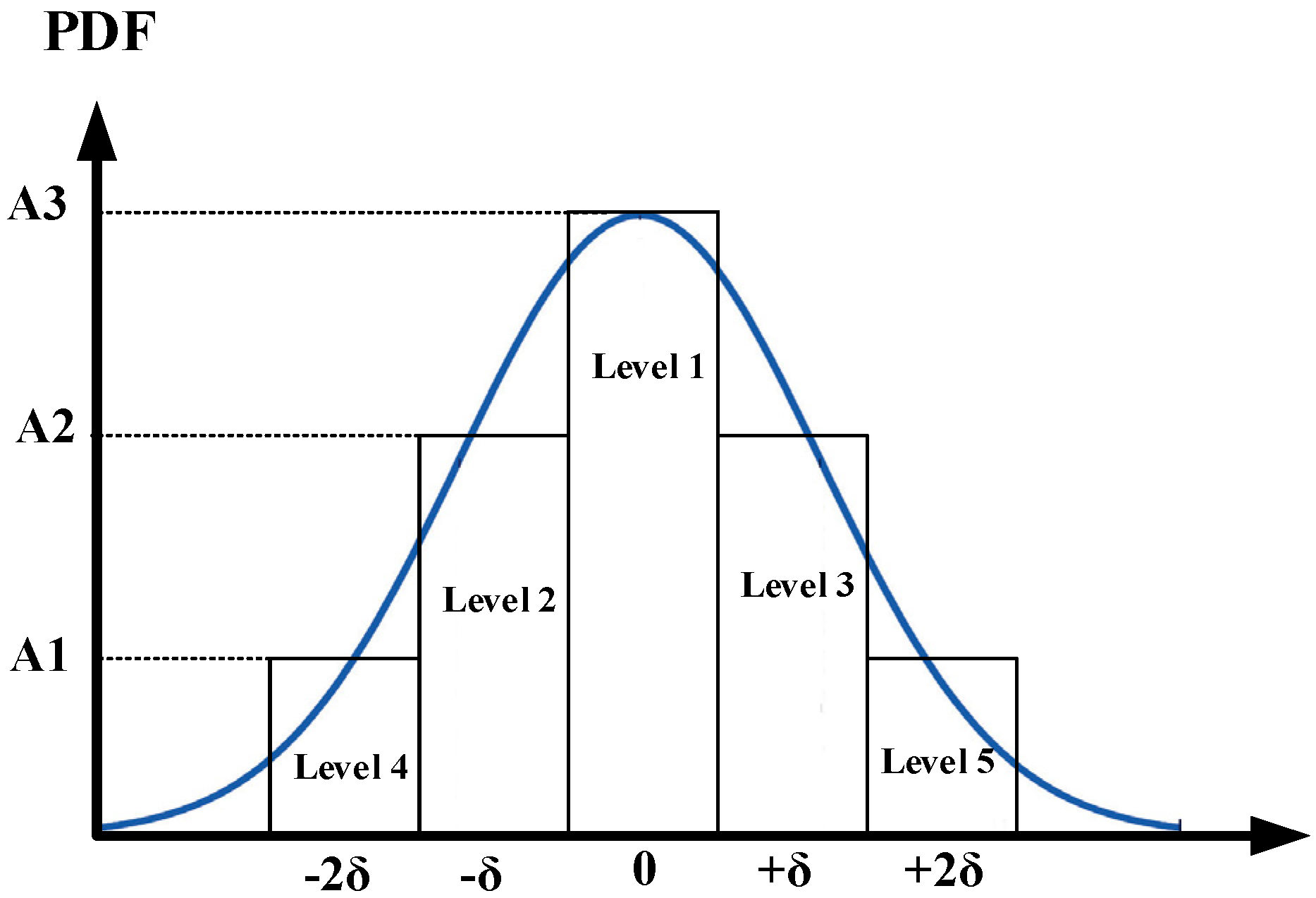
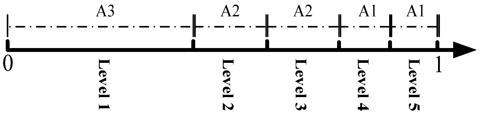
3.3. Scenario Generation

Fitness proportionate selection is one of the most popular ways of parent selection. The general idea is that every individual can become a parent with a probability which is proportional to its fitness. Therefore, fitter individuals have a higher chance of mating and propagating their features to the next generation. Such a selection strategy favors the more fit individuals in the population, resulting in better individuals over time. In our approach first the PDF is divided into several probability levels based on the required precision. Each of them represents the error rate on that section. For example, the PDF in Figure 2 is divided into 5 levels.

To provide each probability level with a random variable to select potentially useful solutions for recombination, the roulette wheel selection algorithm [43] is used (Figure 3). In a roulette wheel selection, a circular wheel is given that is divided into n pies, where n is the number of individuals in the population. Each individual gains a portion of the circle which is proportional to its fitness value. A fixed point is chosen on the wheel circumference and the wheel is rotated. The region of the wheel which comes in front of the fixed point is chosen as the parent.

In Figure 3, the roulette wheel was divided into 5 pies according to the levels considered in the PDF. The intended length for level 1 is A3, which is 70% of the total length of the line. The intended length for Level 2 and Level 3 is A2, which is 10% of the total length of the line and the length for the level 4 and level 5 is equal to A1, which is 5% of the total length of the line. As shown in Figure 3, the sum of the probabilities of the levels is equal to one.

First, a random number with a normal distribution is selected in the interval [0,1]. Then, depending on the obtained value, the appropriate part of the roulette-wheel is selected. This selection process is repeated every hour; e.g., as the level 1 is greater, the probability of choosing level 1 is higher than the other levels.

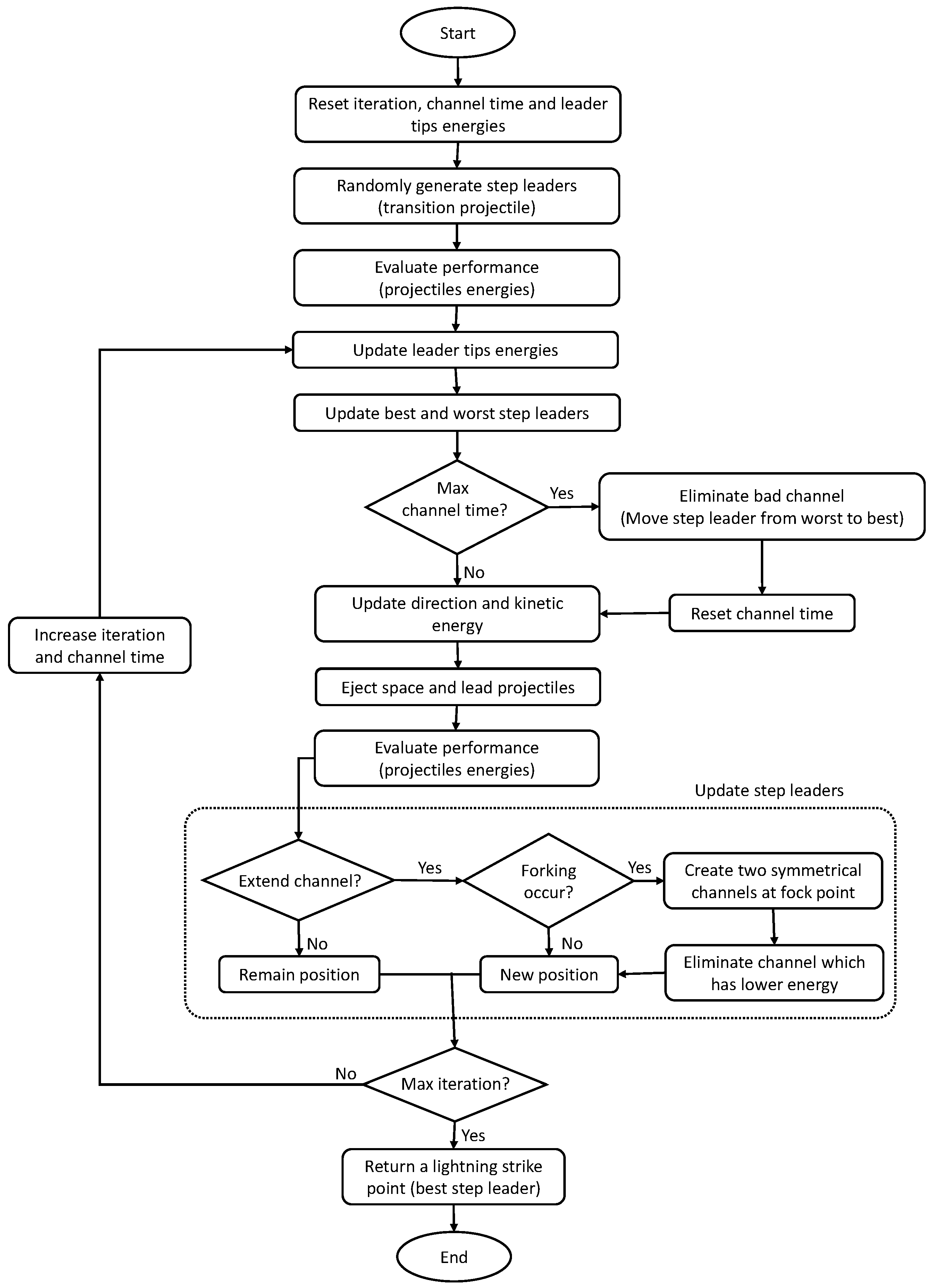
4. Lightning Search Algorithm (LSA)

The lightning search algorithm (LSA), which was first introduced in [44,45], is an effective metaheuristic optimization method for solving real-valued numerical optimization problems. LSA was inspired by the natural phenomenon of lightning and the mechanism of step leader propagation. LSA generalizes the mechanism of step leader propagation. It defines its search space on the basis of a probabilistic movement of a fast particle, named a projectile, in a lightening event; i.e., it considers the involvement of this projectile in the formation of the binary tree structure of the step leader and in the concurrent formation of two leader tips at fork points instead of a conventional step leader mechanism. Similar to other metaheuristics algorithms, the LSA needs a population to begin the search. Projectiles which are similar to the particles concept in PSO, suggest random solutions to solve the problem by the lightning search algorithm. A projectile loses its kinetic energy through movement in the atmosphere. The velocity of a projectile and its kinetic energy are displayed as follows [44,46]:

$$v_p={\left[1-{(1/\sqrt{1-{(v_0/c)}^2}-s{F}_i/m{c}^2)}^{-2}\right]}^{-0.5}$$

(15)

$$E_p=\left(\left(1/\sqrt{1-{(v_p/c)}^2}\right)-1\right)m{c}^2$$

(16)

where $v_0$ is initial speed; $m$ is the mass and $c$ is the light speed; $s$ is the traveled path and $F_i$ is the rate of ionization. The smaller mass of a projectile and shorter path traveled means the larger space it can explore, as the velocity and the ionization ability are higher. Hence, the relative energy of the step leaders determines the power of exploration and the utilization capacity of the LSA. The algorithm uses three different types of particles. The transition projectile begins to populate the search for solutions. The space and lead projectiles are engaged in exploration and they attempt to find and exploit the optimal solution. This results in three different search methods that are deployed. Exponential random behavior is executed by the space projectile that attempts to become the step leader. Opposition theory is used to realize the concurrent formation of two leader tips at fork points. Finally, local search is conducted by the lead projectile that is meant to represent the best positioned projectile that originated from a number N of step leaders [44,46]. In Equation (17), a random variable $x^T$ modeled by uniform PDF, expresses an ejected projectile in a random direction.

$$f\left(x^T\right)=\{\begin{array}{cc}1/b-a\hfill & \hfill a\le x^T\le b\\ 0\hfill & \hfill x^T<a\left|\right|x^T>b\end{array}$$

(17)

where $a$ and $b$ are lower and upper bounds of solution space. The next step after initializing the required solution space is for the projectiles to ionize the vicinity of their old step leaders. This can be modelled by creating a random number using exponential probability density function:

$$f\left(x^S\right)=\{\begin{array}{ll}\frac{1}{\mu }{e}^{\frac{-x^S}{\mu }}& x^S\ge 0\\ 0& x^S<0\end{array}$$

(18)

where $\mu$ is the shaping parameter of the exponential PDF. The new position of the space projectile can be determined by Equation (19), in which $\mathrm{e}xpRand$ is an exponential random number and $P_i^S$ is the old position of space projectiles. The most extended projectile will be the new lead projectile.

$$P_{i\_new}^S=P_i^S\pm \mathrm{e}xpRand\left({\mu }_i\right)$$

(19)

The closest projectiles to the Earth have the least potential to extend the tips, therefore, they can be modelled by creating a random number using normal probability density function.

$$f\left(x^L\right)=\frac{1}{\sigma \sqrt{2\pi }}{e}^{\frac{-{(x^L-\mu )}^2}{2{\sigma }^2}}$$

(20)

As the lead projectile $P^L$ finds the best solution or move toward the Earth, the scale parameter $\sigma$ exponentially decreases. The new position of the lead projectile can be modeled as Equation (21), in which $\mathrm{n}ormRand$ is a random number created by normal PDF and $P_i^L$ is Position of the old lead projectile [44]. In order to improve the performance of the LSA algorithm, a damping rate is added. The value of damping coefficient is dynamic, and it is 0.9 for initial iteration and 0.2 for last iteration.

$$P_{i\_new}^L=P_i^L\pm D\times \mathrm{n}ormRand\left({\mu }_L,{\sigma }_L\right)$$

(21)

LSA proved to have a higher conversion rate than other nature inspired metaheuristic algorithms. Figure 4 illustrates the steps of the LSA in a flowchart.

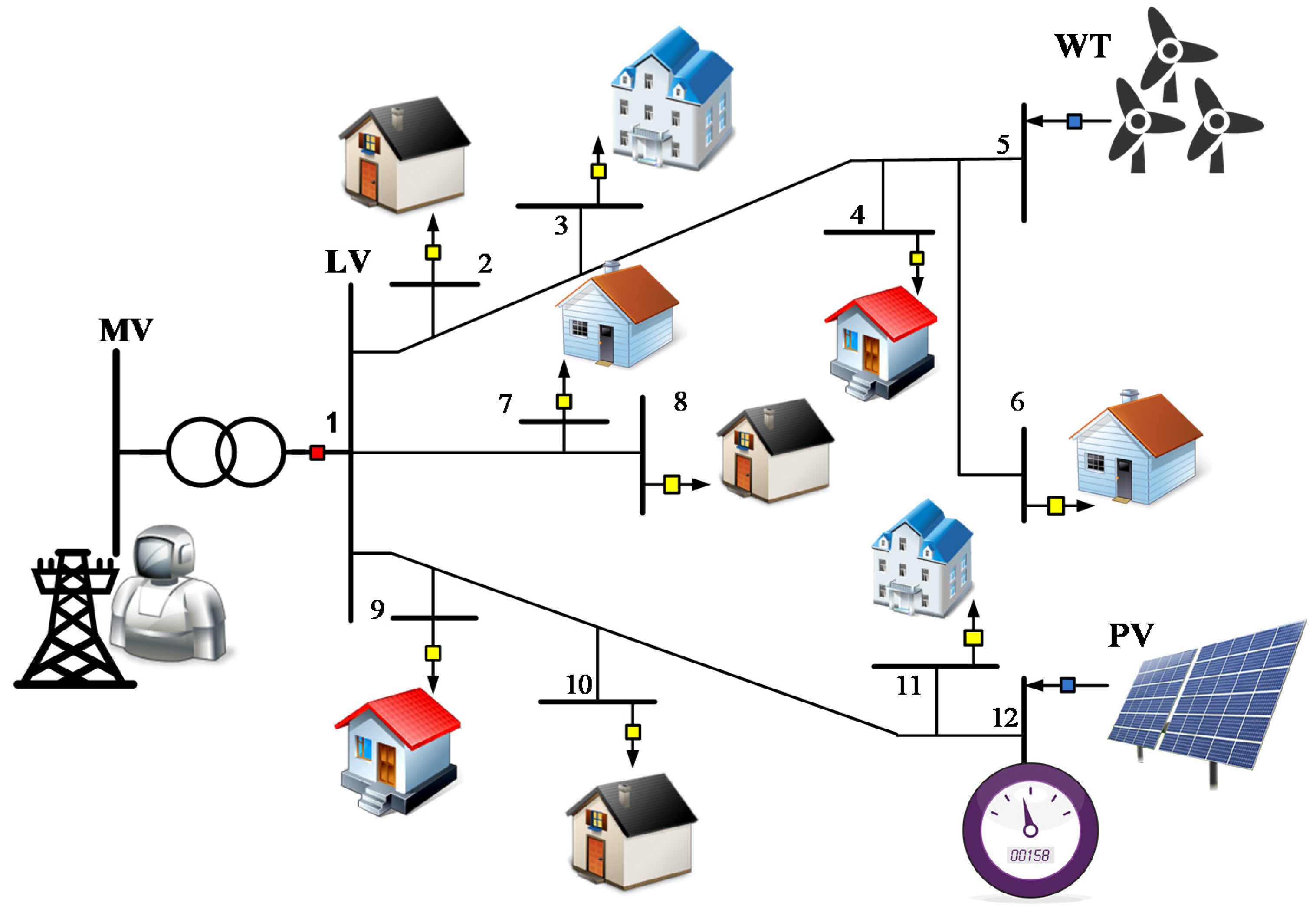
5. Case Study: Microgrid System Model

The model of the underlying microgrid is illustrated in Figure 5. This system is connected to the grid via a 20 KV/0.4 KV transformer to continuously exchange power. The household model includes sensitive loads, adjustable loads and dynamic loads. Obviously, load as the most probable variable of uncertainty plays a very important role in the performance of the power system. Moreover, time and weather are two major factors for the definitive component of demand changes. Daily and weekly changes in demand depend on the behavior of patterns of different energy consumers. In this network, photovoltaic panels and wind turbines are used as EGs. A 100 KW PV panel and a 70 KW wind turbine are installed in the underlaying microgrid. The PV can generate nominal power only if solar irradiation is 1000 w/m². The maximum wind turbine power will be obtained if the wind speed is between the rated and the cut-out speed. The minimum output power of these two resources is zero.

The forecasted daily consumption of households for 24 h is shown in Figure 6a in the early hours, the consumption of households is at the minimum level of 50 KW. At peak hours it can reach up to 200 KW. In order to forecast the daily energy demand, an appropriate PDF is selected, and its parameters are determined using the consumption data of the last days. Then for the upcoming days, the amount of daily consumption for each hour is forecasted by the load PDF.

The price of the power exchanged with the main grid is considered as Time-of-Use (TOU) price, which is shown in Figure 6b. Various scenarios for TOU pricing can be considered. But the one that encourages consumers to shift their consumption to non-peak hours with the low-cost electricity is acceptable, since it can maximize the profitability. The minimum price of power is less than 2 cents per kilowatt and the maximum is 40 cents per kilowatt. As mentioned earlier the power produced by PVs depends on the intensity of the radiation by the sun and the ambient temperature. The predicted values of those two parameters are shown in Figure 7. According to Figure 7b, solar power extraction is only possible from 8 a.m. to 18 p.m., and for the rest of the day, due to the lack of radiation intensity, the PV power output will be zero. The maximum intensity of the radiation of the sun in the studied region at 12 o’clock is approximately 1000 watts per square meter. The ambient temperature also varies from 15 to 30 °C.

Moreover, as the wind turbine output power is influenced by the wind speed in the region, a wind speed forecast is required (Figure 8). The minimum wind speed in the studied region is about 6 m/s and its maximum speed is about 11 m/s.

6. Simulation Result

In this paper, the energy management of the microgrid under load and generation uncertainty is performed by utilizing PSO and LSA. The parameters of these two algorithms are shown in

Table 1. Selected parameters for particle swarm optimization (PSO) and LSA.

LSA	Population	Iteration	α	β	γ
	100	50	0.2	0.8	0.2
PSO	Population	Iteration	C1 = C2	Vmax	Vmin	W
	100	50	2	0.4	0.9	0.7

. We tried to select the parameters so that their performance can be fairly compared.

It is worth mentioning that, different algorithms were used. However, their results were neglected to avoid redundancy. Only the results of the PSO are accumulated in the paper due to its better performance, as well as its similarity to the LSA. The optimization is done by optimal utilization of resources as well as load curtailment in different hours of a day. Simulations are repeated in two parts. In the first part, the optimization is carried out with assumption of certainty in the data of radiation intensity, wind speed and the load, whereas in the second part, simulation is repeated with uncertainty consideration. The overall roadmap for microgrid energy management is as follows:

Step 1:

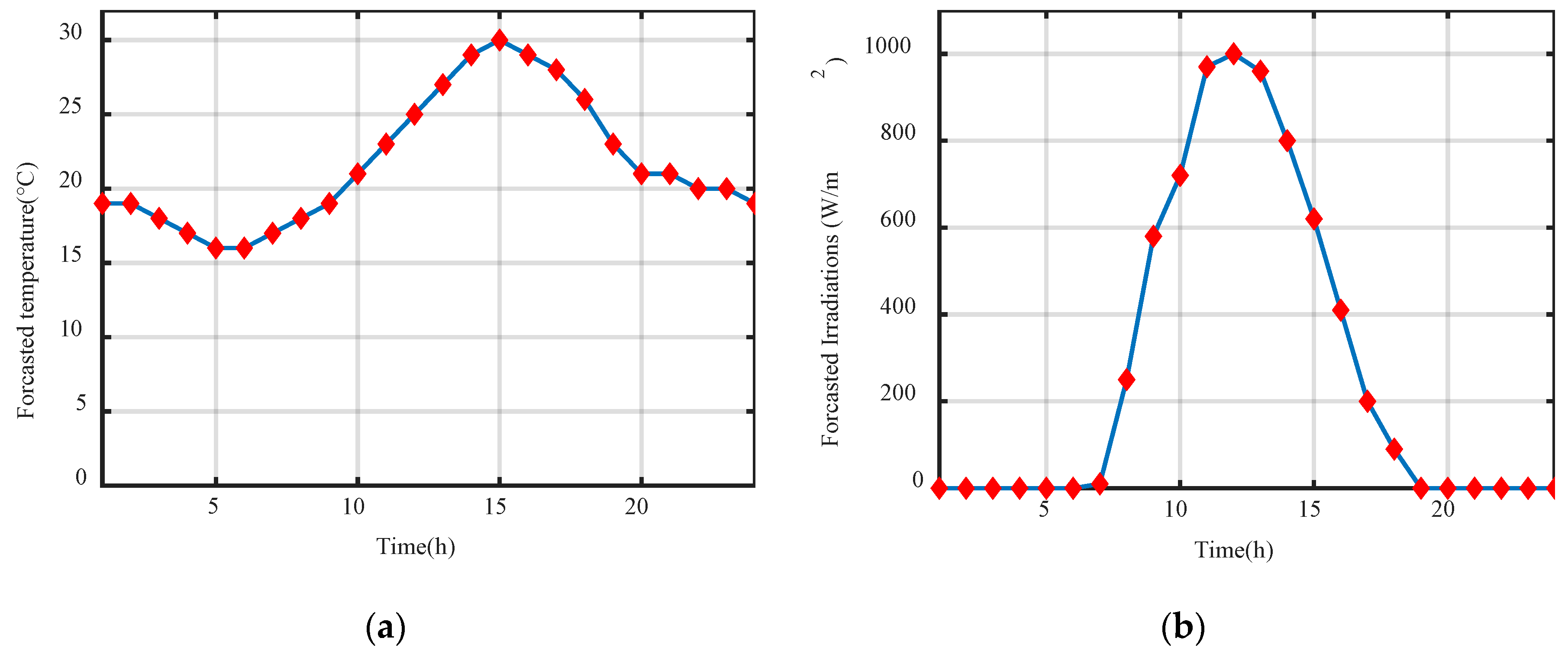
Collecting the solar radiation, the wind speed and the load data in the microgrid.

Step 2:

Selecting the appropriate PDF for the variables (irradiation, wind speed and load) using the values obtained in step one.

Step 3:

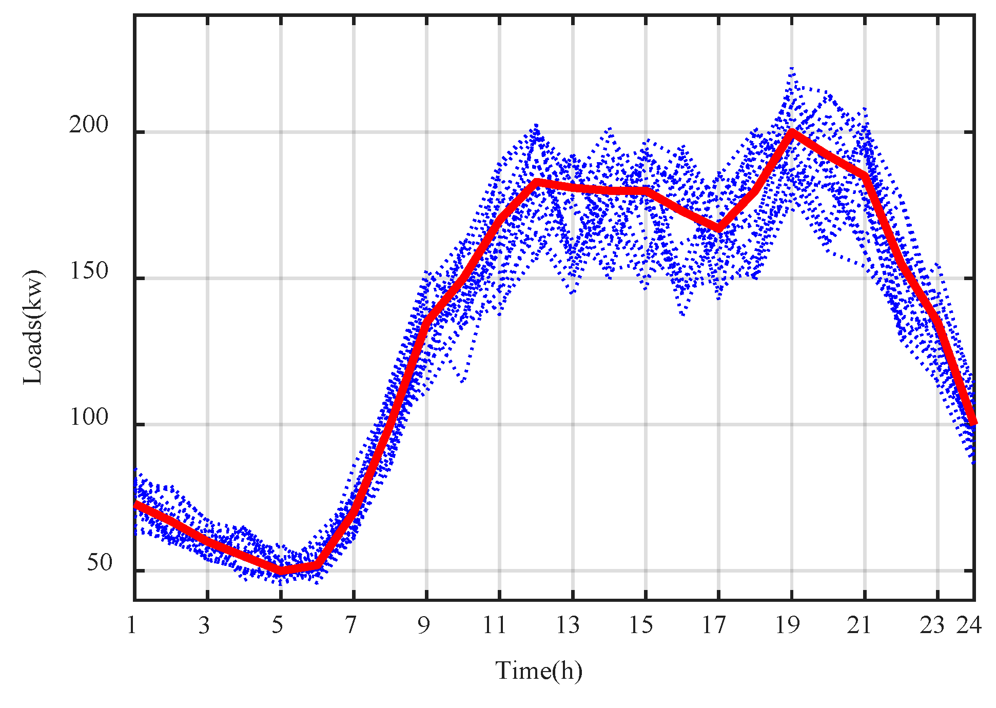
Generating random data for the irradiations, the wind speed, and the load using the PDFs designed in step two.

Step 4:

Selecting scenarios using the roulette wheel mechanism.

Step 5:

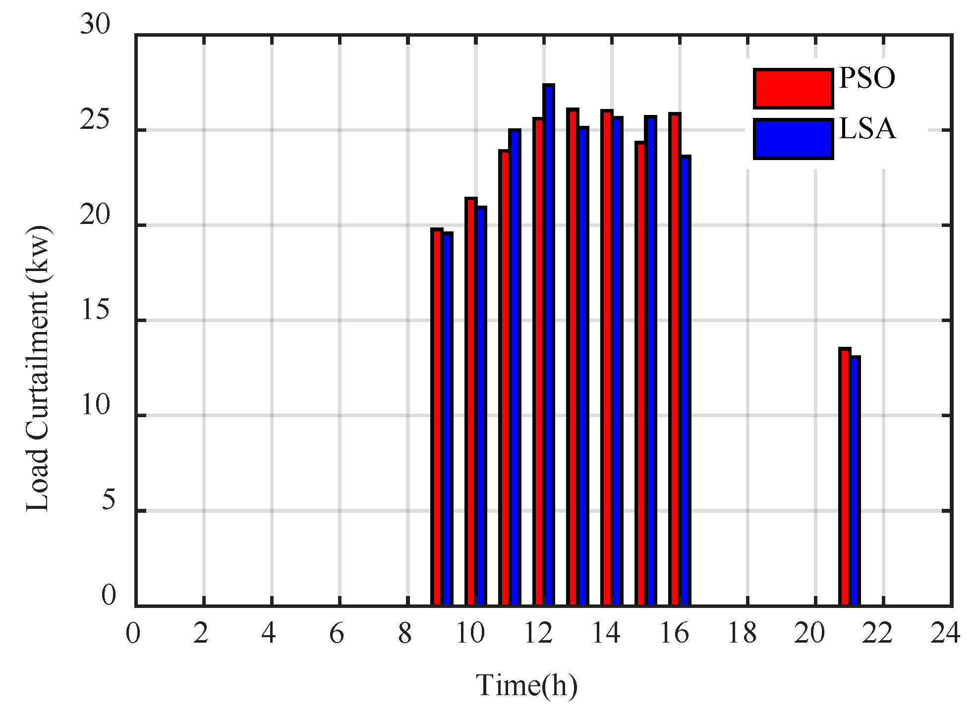
Calculating the optimal microgrid energy management by deploying the modified version of LSA algorithm and using the proposed objective function.

6.1. Part One: Optimization Regardless of Uncertainty

In the first scenario, the optimal utilization of the microgrid is accomplished by reducing the cost through resource management, as well as shedding a part of load, PSO and LSA. Each of the algorithms was executed 20 times (20 trials). In Figure 9, optimization results are shown in 20 different runs of the two algorithms.

In Figure 9, the values of the best solution for 20 trials of the algorithms are shown. All the results (costs) obtained by the LSA are less than the PSO results. Additionally, the LSA responses are closer to each other. The lowest and the highest costs after optimization by the LSA is obtained with 1467.4 € in the fourth trial and 1472.1 € in the 18th trial. While the costs after optimization by the PSO are changed in the broader range. The lowest cost for the PSO is achieved in the seventh trial and it is about 1504.7 €. The worst solution for the PSO is 1518.3 € which is obtained in the third trial.

The best, worst, mean and standard deviation in the first scenario are calculated and presented in

Table 2. Optimization results the first scenario (20 trials).

	Best (€)	Worst (€)	Average (€)	SD
PSO	1504.7	1518.3	1509.7	6.67
LSA	1467.4	1472.1	1470.6	2.41

.

According to the Table 2, the best responses in performing 20 trials of the PSA and LSA algorithms are estimated to be 1504.7 € and 1467.4 €, respectively, while the worst responses for these two algorithms are 1518.3 € and 1472.1 €. The average response of the PSO algorithm is 1509.7 € and the average response of the LSA algorithm is 1470.6 €. The greater deviation of the results of the particle swarm algorithm has led to a standard deviation of 6.67, while the standard deviation of the results of the LSA algorithm is 2.41. The lower standard deviation means the higher proximity of the results obtained in different runs and hence, the higher accuracy of the algorithm. In order to evaluate the effect of the losses on the energy management study, they are changed from 5% to 15%, and the operation cost is calculated. With 5% microgrid losses the cost is 1403.8 €, after the energy management was conducted by the LSA algorithm. If the losses are 15%, the cost of the operation will be 1494.6 €. Figure 10 shows the convergence process of the algorithms to the best response.

As shown in Figure 10, the particle swarm algorithm converges to 1504.7 € after 24 iterations, and the lightning search algorithm has reached a final value of 1467.4 € after 23 iterations. The cost of the microgrid in 24 h in case of the optimal energy management by LSA is approximately 37.3 € lower than those of PSO. The microgrid operational costs are predicted to be about 4711.6 € in the absence of distributed generation and lack of energy management, and only by supplying energy from the main grid. In the presence of solar and wind resources and the demand response ability it drops by approximately 69% using LSA and 68% using PSO. The percentage of cost reduction for the two algorithms is almost the same, which confirms the efficiency of both algorithms. Figure 11 shows the share of distributed generation and the amount of energy purchased from the network in 24 h, optimized by LSA and PSO.

In Figure 11, the blue bars, are the amount of load per hour. The red bars show the energy demand after the load curtailment by the algorithm. Orange and violet bars are the amount of power produced by solar and wind, respectively. Finally, the green bars indicate the amount of electrical energy exchanged with the upstream network. As expected, to reduce the cost of the microgrid utilization, in the time of higher energy prices, the required power is going to be mostly provided by PV and WT, whereas in the time of cheaper price most of the required energy is purchased from the main grid. At 10, 11, 12, and 14, the amount of power exchanged is negative, indicating that electricity is supplied to the upstream network to increase profitability. The profitability of electricity sales in these four hours is about 500 €. At peak hours, due to the high price of electrical energy, solar and wind resources are injected into the network at their maximum capacity. It should be noted that the maximum allowed load curtailment is 15% of the total load at the same hour which is usually done at peak hours of consumption. The amount of load curtailment in each hour is shown in Figure 12.

The load curtailment has occurred between 9 to 16, due to the higher price of electrical energy at those hours. The maximum load curtailment is less than 30 KW per hour. Discarding uncertainties causes the simulation result not to have enough executive guarantee and the result will be different from the actual value, especially when the sources of uncertainty in the system are high. In this paper, due to the presence of distributed generations, such as wind and solar sources, and their random nature, there is a significant difference between simulation results without considering uncertainties and the real-world values.

6.2. Part Two: Optimization Considering Uncertainties

In this section, the optimal utilization of the microgrid is done, taking into account the uncertainties of solar and wind power as well as the load uncertainty. First, 50 scenarios of solar radiation intensity, wind speed, and load, were generated using the probability distribution functions described in Section 3.3, Solar and wind power outputs in various scenarios are shown in Figure 13.

In Figure 13, the forecasted power is shown by the bold red line and the power output of various scenarios are shown with blue points. The maximum difference between the forecasted output power of EGs and the scenarios is in the finite range. The maximum deviation for solar power ranges from −24.3 kilowatt to 25.36 KW, and for wind power is −24.4 to 25.36 KW. Figure 14 shows the amount of electrical energy requested by households over a period of 24 h in different scenarios.

The difference between the predicted demand and the loads estimated by scenarios is in the finite range of −36.8 KW in hour 13, and 32.8 KW in hour 20. The PSO and LSA are used to manage the resource energies and determine the amount of load curtailment.

In the presence of uncertainty, PSO and LSA were run 20 times, and the best, worst, mean, and standard deviation is calculated. The results obtained by the optimization are presented in

Table 3. Optimization results for 20 trials in part 2.

Scenario	Algorithm	Best (€)	Worst (€)	Average (€)	SD	Simulation Time (s)
S1	PSO	1546.3	1572.7	1564.6	5.43	64.33
	LSA	1534.4	1543.1	1537.2	2.82	57.41
S2	PSO	1764.2	1791.3	1778.2	6.43	67.24
	LSA	1758.1	1771.2	1765	2.72	59.23
S3	PSO	1521.6	1546.5	1534.9	5.14	65.84
	LSA	1507.5	1518.4	1512.2	2.63	58.26
S4	PSO	1842.6	1876.9	1864.7	7.77	65.56
	LSA	1833.4	1842.2	1837.9	3.13	57.44
S5	PSO	1661.7	1686.3	1674.3	6.23	65.72
	LSA	1632.1	1638	1635.5	2.34	58.69
S6	PSO	1573.2	1597.4	1589.4	5.89	66.82
	LSA	1560.2	1569.7	1565.3	2.38	53.67
S7	PSO	1612.6	1646.5	1638.3	7.21	67.42
	LSA	1601.7	1612.2	1607.2	2.89	56.48
S8	PSO	1586.3	1612.8	1603.3	5.78	62.91
	LSA	1552.2	1561.1	1556.9	2.42	58.32
S9	PSO	1723.4	1748.3	1737	7.86	68.22
	LSA	1696.3	1708.4	1701.4	3.07	57.69
S10	PSO	1573.1	1598.6	1589.5	5.94	63.83
	LSA	1541.9	1550.8	1546.8	2.63	54.76

.

Given the uncertainties, different cost amounts in different scenarios are obtained by varying the demand and solar and wind power outputs. There is a significant difference between costs due to the uncertainty in production and consumption. The cost difference between the third and the fourth scenario is more than 320 €. The lowest cost is obtained in scenarios in which the demand was rather low; i.e., when it is possible to sell electricity to the upstream network. The minimum cost in ten scenarios is obtained in scenario S3, which is estimated 1521.6 € for the PSO algorithm and 1507.5 € for the LSA algorithm. The maximum cost of the microgrid in the defined scenarios, if optimized by the PSO algorithm, is equal to 1842.6 € and, if optimized by the LSA algorithm, is calculated at 1833.4 €. The standard deviations of the responses obtained by both algorithms are rather small, but the standard deviations in the responses of the proposed LSA are roughly half of the standard deviations of the PSO algorithm, which confirms the high accuracy of the proposed LSA.

In the following, the amount of power generated by EGs along with the amount of energy purchased from the network in 24 h, is optimized by PSO and LSA. Figure 15 and Figure 16 show the results obtained for the third (S3) and fourth (S4) scenarios, respectively.

In scenario 3, the electrical energy demanded by subscribers is smaller compared to the predicted values, while the solar and wind power output is higher. In this situation, there is the possibility of exchanging more power with the upstream network; i.e., more energy can be sold by the microgrid operator agent for a better price to the upstream network. Such favorable situations exist at peak times, especially from 10 to 14. The cost of scenario 3 in the absence of demand response and without utilization of distributed generation resources is 3675 €. After energy management by the LSA, the cost decreases by 59%. Using the PSO algorithm, the cost decreases by 58.6%.

The existence of uncertainty in the microgrid can create additional costs for the operator. The maximum current cost in the microgrid is when the electrical energy demand in the grid is high. Under these circumstances, costs have risen due to lower energy sales. It should be noted that in this case, the cost of the microgrid operation is estimated to be 5701.5 € in the absence of any energy management. The optimal energy management by the PSO algorithm eliminates 67.7% of the costs, and the LSA optimization leads to 67.9% cost reduction. Although costs in the scenario 4 have increased due to the system’s increased load, the percentage of cost savings in this scenario is higher than the scenario 3.

7. Conclusions

If energy management within a microgrid is not properly handled, the reliability of the system will suffer and costs will increase. Several methods have been used for the energy management under uncertainty, among which, the most suitable one is the use of metaheuristic algorithms with an appropriate objective function. In this paper, the optimal utilization of a microgrid using the modified version of the lightning search algorithm is studied, considering the load and distributed generation uncertainties. First, using the preset information of radiation intensity, wind speed, and microgrid load, the suitable probability density function was chosen for each of them. Then, various scenarios of power generation by EGs, as well as microgrid loads were generated, using PDFs. A weighting objective function based on the cost of the microgrid is presented, in which each scenario is weighted according to its probability of occurrence. The proposed objective function had a significant influence on the energy management. The probable scenarios had greater impact and the unlikely ones had less impact on the objective function. Finally, in addition to the modified version of the lightning search algorithm, a particle swarm optimization algorithm was used to manage the microgrid grid and the demand response program. The optimization results in different scenarios indicate that in case of having uncertainty, grid costs are subject to variations within a certain range, depending on the microgrid load and the outputs of EGs. With the proper energy management, the microgrid cost is reduced more than 65%. Also, it is shown that the proposed modified LSA has a better performance compared to the PSO algorithm and reduces the cost of utilizing the microgrid to a greater extent. In future work, the proposed multi-agent-based approach for microgrid energy management will be extended by energy storage facilities. The intermittent nature of renewable power generation cannot be tackled by a sophisticated demand and supply management only. The unpredictable power generation as well as the non-stable/non-continuous production of renewable energy (e.g., the problem of photovoltaics and no sunlight (at nights)) requires substantial storage facilities for energy that need to exceed the current storage facilities by far. Thus, the impact of using energy storage on the complexity of the energy management problem under uncertainty, as well as its impact on the overall profitability will be examined. We hope to obtain ideas about what a good compromise between the investment into storage capabilities; i.e., storage capacities and storage types, and its effects on reliability and costs may look like.

References

1. Hatziargyriou, N.; Asano, H.; Iravani, R.; Marnay, C. Microgrids. IEEE Power Energy Mag. 2007, 5, 78–94. [Google Scholar] [CrossRef]
2. Olivares, D.E.; Mehrizi-Sani, A.; Etemadi, A.H.; Cañizares, C.A.; Iravani, R.; Kazerani, M.; Hajimiragha, A.H.; Gomis-Bellmunt, O.; Saeedifard, M.; Palma-Behnke, R.; et al. Trends in microgrid control. IEEE Trans. Smart Grid. 2014, 5, 1905–1919. [Google Scholar] [CrossRef]
3. Khan, A.A.; Naeem, M.; Iqbal, M.; Qaisar, S.; Anpalagan, A. A compendium of optimization objectives, constraints, tools and algorithms for energy management in microgrids. Renew. Sustain. Energy Rev. 2016, 58, 1664–1683. [Google Scholar] [CrossRef]
4. Feng, W.; Jin, M.; Liu, X.; Bao, Y.; Marnay, C.; Yao, C.; Yu, J. A review of microgrid development in the United States—A decade of progress on policies, demonstrations, controls, and software tools. Appl. Energy 2018, 228, 1656–1668. [Google Scholar] [CrossRef]
5. Pourbehzadi, M.; Niknam, T.; Aghaei, J.; Mokryani, G.; Shafie-khah, M.; Catalão, J.P. Optimal operation of hybrid AC/DC microgrids under uncertainty of renewable energy resources: A comprehensive review. Int. J. Electr. Power Energy Syst. 2019, 109, 139–159. [Google Scholar] [CrossRef]
6. Zia, M.F.; Elbouchikhi, E.; Benbouzid, M. Microgrids energy management systems: A critical review on methods, solutions, and prospects. Appl. Energy. 2018, 222, 1033–1055. [Google Scholar] [CrossRef]
7. Dong, G.; Chen, Z. Data-driven energy management in a home microgrid based on bayesian optimal algorithm. IEEE Trans. Ind. Inform. 2019, 15, 869–877. [Google Scholar] [CrossRef]
8. Ju, C.; Wang, P.; Goel, L.; Xu, Y. A two-layer energy management system for microgrids with hybrid energy storage considering degradation costs. IEEE Trans. Smart Grid 2018, 9, 6047–6057. [Google Scholar] [CrossRef]
9. Moradi, H.; Esfahanian, M.; Abtahi, A.; Zilouchian, A. Optimization and energy management of a standalone hybrid microgrid in the presence of battery storage system. Energy 2018, 147, 226–238. [Google Scholar] [CrossRef]
10. Ghorbani, S.; Unland, R. A Holonic Multi-Agent Control System for Networks of Micro-Grids. In Proceedings of the German Conference on Multiagent System Technologies, Klagenfurt, Austria, 27–30 September 2016; Springer: Cham, Switzerland, 2016; pp. 231–238. [Google Scholar]
11. Meng, L.; Sanseverino, E.R.; Luna, A.; Dragicevic, T.; Vasquez, J.C.; Guerrero, J.M. Microgrid supervisory controllers and energy management systems: A literature review. Renew. Sustain. Energy Rev. 2016, 60, 1263–1273. [Google Scholar] [CrossRef]
12. Vrba, P.; Mařík, V.; Siano, P.; Leitão, P.; Zhabelova, G.; Vyatkin, V.; Strasser, T. A review of agent and service-oriented concepts applied to intelligent energy systems. IEEE Trans. Ind. Inform. 2014, 10, 1890–1903. [Google Scholar] [CrossRef]
13. Esfahani, M.M.; Hariri, A.; Mohammed, O.A. A multiagent-based game-theoretic and optimization approach for market operation of multimicrogrid systems. IEEE Trans. Ind. Inform. 2019, 15, 280–292. [Google Scholar] [CrossRef]
14. Liu, W.; Gu, W.; Wang, J.; Yu, W.; Xi, X. Game Theoretic Non-Cooperative Distributed Coordination Control for Multi-Microgrids. IEEE Trans. Smart Grid 2018, 9, 6986–6997. [Google Scholar] [CrossRef]
15. Arcos-Aviles, D.; Guinjoan, F.; Pascual, J.; Marroyo, L.; Sanchis, P.; Gordillo, R.; Ayala, P.; Marietta, M.P. A review of fuzzy-based residential grid-connected microgrid energy management strategies for grid power profile smoothing. In Energy Sustainability in Built and Urban Environments; Springer: Cham, Switzerland, 2019; pp. 165–199. [Google Scholar]
16. Hettiarachchi, H.; Hemapala, K.U.; Jayasekara, A.B.P. Review of applications of fuzzy logic in multi-agent-based control system of ac-dc hybrid microgrid. IEEE Access 2019, 7, 1284–1299. [Google Scholar] [CrossRef]
17. Faisal, M.; Hannan, M.A.; Ker, P.J.; Hussain, A.; Mansor, M.B.; Blaabjerg, F. Review of energy storage system technologies in microgrid applications: Issues and challenges. IEEE Access 2018, 6, 35143–35164. [Google Scholar] [CrossRef]
18. Morsali, R.; Ghorbani, S.; Kowalczyk, R.; Unland, R. On battery management strategies in multi-agent microgrid management. In Proceedings of the International Conference on Business Information Systems, Poznan, Poland, 28–30 June 2017; Springer: Cham, Switzerland, 2017; pp. 191–202. [Google Scholar]
19. Haider, H.T.; See, O.H.; Elmenreich, W. A review of residential demand response of smart grid. Renew. Sustain. Energy Rev. 2016, 59, 166–178. [Google Scholar] [CrossRef]
20. Strüker, J. Blockchain-based management of shared energy assets using a smart contract ecosystem. In Proceedings of the Business Information Systems Workshops: BIS 2018 International Workshops, Seville, Spain, 26–28 June 2019; Revised Papers. Springer: Cham, Switzerland, 2019; p. 217. [Google Scholar]
21. Imani, M.H.; Ghadi, M.J.; Ghavidel, S.; Li, L. Demand response modeling in microgrid operation: A review and application for incentive-based and time-based programs. Renew. Sustain. Energy Rev. 2018, 94, 486–499. [Google Scholar] [CrossRef]
22. Ghorbani, S.; Rahmani, R.; Unland, R. Multi-agent Autonomous Decision Making in Smart Micro-Grids’ Energy Management: A Decentralized Approach. In Proceedings of the German Conference on Multiagent System Technologies, Leipzig, Germany, 23–26 August 2017; Springer: Cham, Switzerland, 2017; pp. 223–237. [Google Scholar]
23. Ghorbani, S.; Morsali, R.; Unland, R.; Kowalczyk, R. Distributed multi-agent based energy management of smart micro-grids: Autonomous participation of agents in power imbalance handling. In Proceedings of the International Conference on Practical Applications of Agents and Multi-Agent Systems, Toledo, Spain, 20–22 June 2018; Springer: Cham, Switzerland, 2018; pp. 321–332. [Google Scholar]
24. Gholami, K.; Dehnavi, E. A modified particle swarm optimization algorithm for scheduling renewable generation in a micro-grid under load uncertainty. Appl. Soft Comput. 2019, 78, 496–514. [Google Scholar] [CrossRef]
25. Indragandhi, V.; Logesh, R.; Subramaniyaswamy, V.; Vijayakumar, V.; Siarry, P.; Uden, L. Multi-objective optimization and energy management in renewable based AC/DC microgrid. Comput. Electr. Eng. 2018, 70, 179–198. [Google Scholar]
26. Roy, K.; Mandal, K.K.; Mandal, A.C. Ant-Lion Optimizer algorithm and recurrent neural network for energy management of micro grid connected system. Energy 2019, 167, 402–416. [Google Scholar] [CrossRef]
27. Xu, M.; Gu, T.; Qin, J.; Zheng, W. GA Based Multi-Objective Operation Optimization of Power Microgrid. In Proceedings of the 2019 IEEE International Conference on Intelligent Transportation, Big Data & Smart City (ICITBS), Changsha, China, 12–13 January 2019; pp. 103–107. [Google Scholar]
28. Shan, H.; Hongjing, L.; Linlin, W.; Feng, Z.; Wang, M.; Yang, L.; Jie, G. Economic optimisation of microgrid based on improved quantum genetic algorithm. J. Eng. 2019, 2019, 1167–1174. [Google Scholar] [CrossRef]
29. Agüera-Pérez, A.; Palomares-Salas, J.C.; de la Rosa, J.J.G.; Florencias-Oliveros, O. Weather forecasts for microgrid energy management: Review, discussion and recommendations. Appl. Energy 2018, 228, 265–278. [Google Scholar] [CrossRef]
30. Maleki, A.; Khajeh, M.G.; Ameri, M. Optimal sizing of a grid independent hybrid renewable energy system incorporating resource uncertainty, and load uncertainty. Int. J. Electr. Power Energy Syst. 2016, 83, 514–524. [Google Scholar] [CrossRef]
31. Roy, A.; Kedare, S.B.; Bandyopadhyay, S. Optimum sizing of wind-battery systems incorporating resource uncertainty. Appl. Energy 2010, 87, 2712–2727. [Google Scholar] [CrossRef]
32. Fazlalipour, P.; Ehsan, M.; Mohammadi-Ivatloo, B. Optimal participation of low voltage renewable micro-grids in energy and spinning reserve markets under price uncertainties. Int. J. Electr. Power Energy Syst. 2018, 102, 84–96. [Google Scholar] [CrossRef]
33. Aien, M.; Hajebrahimi, A.; Fotuhi-Firuzabad, M. A comprehensive review on uncertainty modeling techniques in power system studies. Renew. Sustain. Energy Rev. 2016, 57, 1077–1089. [Google Scholar] [CrossRef]
34. Mohseni-Bonab, S.M.; Rabiee, A.; Mohammadi-Ivatloo, B. Voltage stability constrained multi-objective optimal reactive power dispatch under load and wind power uncertainties: A stochastic approach. Renew. Energy 2016, 85, 598–609. [Google Scholar] [CrossRef]
35. Shargh, S.; Mohammadi-Ivatloo, B.; Seyedi, H.; Abapour, M. Probabilistic multi-objective optimal power flow considering correlated wind power and load uncertainties. Renew. Energy 2016, 94, 10–21. [Google Scholar] [CrossRef]
36. Yang, Y.; Li, S.; Li, W.; Qu, M. Power load probability density forecasting using Gaussian process quantile regression. Appl. Energy 2018, 213, 499–509. [Google Scholar] [CrossRef]
37. Koohi-Kamali, S.; Rahim, N.A.; Mokhlis, H. Smart power management algorithm in microgrid consisting of photovoltaic, diesel, and battery storage plants considering variations in sunlight, temperature, and load. Energy Convers. Manag. 2014, 84, 562–582. [Google Scholar] [CrossRef]
38. Teng, J.-H.; Luan, S.-W.; Lee, D.-J.; Huang, Y.-Q. Optimal charging/discharging scheduling of battery storage systems for distribution systems interconnected with sizeable PV generation systems. IEEE Trans. Power Syst. 2012, 28, 1425–1433. [Google Scholar] [CrossRef]
39. Tito, S.; Lie, T.; Anderson, T. Optimal sizing of a wind-photovoltaic-battery hybrid renewable energy system considering socio-demographic factors. Sol. Energy 2016, 136, 525–532. [Google Scholar] [CrossRef] [Green Version]
40. Fan, X.; Wang, W.; Shi, R.; Cheng, Z. Hybrid pluripotent coupling system with wind and photovoltaic-hydrogen energy storage and the coal chemical industry in Hami, Xinjiang. Renew. Sustain. Energy Rev. 2017, 72, 950–960. [Google Scholar] [CrossRef]
41. Kayal, P.; Chanda, C. Optimal mix of solar and wind distributed generations considering performance improvement of electrical distribution network. Renew. Energy 2015, 75, 173–186. [Google Scholar] [CrossRef]
42. Zhou, B.; Xu, D.; Chan, K.W.; Li, C.; Cao, Y.; Bu, S. A two-stage framework for multiobjective energy management in distribution networks with a high penetration of wind energy. Energy 2017, 135, 754–766. [Google Scholar] [CrossRef]
43. Lipowski, A.; Lipowska, D. Roulette-wheel selection via stochastic acceptance. Phys. A Stat. Mech. Appl. 2012, 391, 2193–2196. [Google Scholar] [CrossRef] [Green Version]
44. Shareef, H.; Ibrahim, A.A.; Mutlag, A.H. Lightning search algorithm. Appl. Soft Comput. 2015, 36, 315–333. [Google Scholar] [CrossRef]
45. Shareef, H.; Mutlag, A.H.; Azah, M. A novel approach for fuzzy logic PV inverter controller optimization using lightning search algorithm. Neurocomputing 2015, 168, 435–453. [Google Scholar] [CrossRef]
46. Islam, M.M.; Shareef, H.; Mohamed, A.; Wahyudie, A. A binary variant of lightning search algorithm: BLSA. Soft Comput. 2017, 21, 2971–2990. [Google Scholar] [CrossRef]
47. Wang, M.Q.; Gooi, H.B. Spinning reserve estimation in microgrids. IEEE Trans. Power Syst. 2011, 26, 1164–1174. [Google Scholar] [CrossRef]
Figure 1. Power curve of a typical wind turbine.
Inventions 04 00037 g001
Figure 2. Probability density function with five level uncertainty.
Inventions 04 00037 g002
Figure 3. Roulette-wheel selection.
Inventions 04 00037 g003
Figure 4. Flowchart of the lightning search algorithm (LSA) [44].
Inventions 04 00037 g004
Figure 5. General view of a microgrid with photovoltaic (PV) solar power and wind turbines (WT).
Inventions 04 00037 g005
Figure 6. (a) The forecasted load for 24 h in the underlying microgrid; (b) time-of-use price for a 24 h period [47].
Inventions 04 00037 g006
Figure 7. Forecasted temperature (a) and radiation intensity (b).
Inventions 04 00037 g007
Figure 8. Wind speed forecast in the region for a 24-h period.
Inventions 04 00037 g008
Figure 9. Optimization results of PSO and LSA in 20 trials.
Inventions 04 00037 g009
Figure 10. The convergence process of PSO and LSA for the first scenario.
Inventions 04 00037 g010
Figure 11. Power produced by PV and WT, and exchanged power with network.
Inventions 04 00037 g011
Figure 12. Load curtailment in each hour.
Inventions 04 00037 g012
Figure 13. WT (a) and PV (b) power outputs in 50 scenarios.
Inventions 04 00037 g013
Figure 14. Forecasted demand and created loads by various scenarios.
Inventions 04 00037 g014
Figure 15. The power produced by energy generation sources (EGs) and the exchanged power with the upstream network in the third scenario (S3).
Inventions 04 00037 g015aInventions 04 00037 g015b
Figure 16. Power produced by EGs and exchanged power with upstream network in forth scenario (S4).
Inventions 04 00037 g016