

Geant4 Simulation of Muon Absorption in Concrete Layers

Department of Physics, Kennesaw State University, Marietta, GA 30060, USA
*
Author to whom correspondence should be addressed.
†
These authors contributed equally to this work.
Instruments 2023, 7(2), 17; https://doi.org/10.3390/instruments7020017
Submission received: 23 March 2023
/
Revised: 15 May 2023
/
Accepted: 29 May 2023
/
Published: 31 May 2023
(This article belongs to the Special Issue Muography, Applications in Cosmic-Ray Muon Imaging)
Abstract
:Muography requires a detailed understanding of the absorption of muons in the material situated between the muon source and the detector. A large-statistics (>3 billion event) Geant4 simulation was run to simulate the absorption of muons in different thicknesses of concrete layers and to determine the effect of the material on the energies of muons that were not absorbed. The Geant4 simulation included a simple detector placed directly behind the absorbing material. A Geant4 simulation was also run for the same detector for alpha sources with no absorbing material and the results of this simulation were compared to the signals from the physical detector built in the laboratory and measured using standard alpha sources. The large-statistics simulations using muons of different energies were compared to the predictions of muon absorption from existing literature. The results of the simulations were in good agreement with both the measured signals from the laboratory as well as the predictions from the literature and the general method is found to be well-suited for studies used for muography involving material layers of uniform thickness.
1. Introduction
Muography is an imaging technique that utilizes the unique properties of subatomic particles called muons passing through the material to achieve a 3D mapping of structures [1,2,3,4,5]. This is made possible by using the flux of cosmic-ray muons that are generated in our upper atmosphere as the muon source. The relativistic speeds of cosmic-ray muons allow them to traverse the atmosphere down to the surface of the earth, and their rate of absorption allows them to travel through dense materials before being detected. The energies and trajectories of the detected muons can then be used to create a density map of the structure of interest.
There are several methods available to detect the muons themselves. One of the simplest of these methods uses the ionization of air molecules produced when the charged muons pass through a volume of air in the presence of an electric field. The ionized air molecules may then be attracted to the positively and negatively charged components of the detector, and the resulting current can then be read out to give a measurement of the rate of ionization [6].
In this paper, we describe a very simple ionization device that is both inexpensive to construct and also capable of detecting muons in a narrow energy band that can itself be predicted via simulation. We first describe a simulation of the ionization detector for alpha particles, which was validated in the laboratory and for which the predicted and measured detection capabilities were found to be in good agreement. We then describe an extension of the validated simulation to muons and show that the detectors are capable, in principle, of observing differences in thickness in layers of material placed above them. These material layers absorb some of the energy of the incoming muons and thus change the rate at which muons pass through the detectors in the energy range of peak sensitivity. The results of this simulation are then compared to literature values for muon-stopping power and found to be consistent with them. We also discuss the computing power needed to run the simulation and compare a smaller-scale simulation of 6 million muons with a larger simulation of over 3 billion muons run on a cluster. The overall goal of the study is to accurately simulate the absorption of muons in thin uniform materials using a simulation that has been validated in the laboratory via alpha source measurements. It is hoped that this study can be of use to the muography community as a potential source of additional information regarding energy absorption in the material above the detectors.
2. Materials and Methods
2.1. Simulation and Detector Geometry
Although our project was primarily simulation-based, we used a detector design that was simple enough that it could be easily constructed in the laboratory to make validation measurements on standard sources which could be compared with the results of the simulation. The validation measurements themselves are discussed in a later section.
Our simulation itself was performed in Geant4, which is short for Geometry and Tracking 4. Geant4 is a Monte-Carlo C++ toolkit for designing detector geometries and simulating particle interactions. It is a well-known software environment and, for further details, the reader is encouraged to refer to the cited literature [7,8,9]. The physics list that was applied to the simulation was G4EmLivermorePhysics, which is an extension of the G4EmStandardPhysics-option4 that includes additional information about photon/electron interactions for energy ranges between 10 ev and 100 GeV [10]. In applying the list the default values for particle production and propagation energy cuts from G4EmLivermorePhysics were used.
2.2. Geant4 Modeling of Detector with Alpha Particles
Our Geant4 simulation was performed with a detector whose geometry was simple enough that it could be easily constructed and validated in the laboratory for standard alpha sources. Although the overall aim is to detect muons, and there are obvious physical differences between alphas and muons, alpha sources provided a test of our ionization detection simulation, which was accessible in our laboratory for validation. The simulations for the alpha sources were run on a desktop environment with CentOS 8, an open source Linux distribution, as the operating system. The hardware components used were an Intel quad-core processor at 4.0 GHz, 16 GB of GDDR4 RAM, and an Nvidia RTX 2060 GPU.
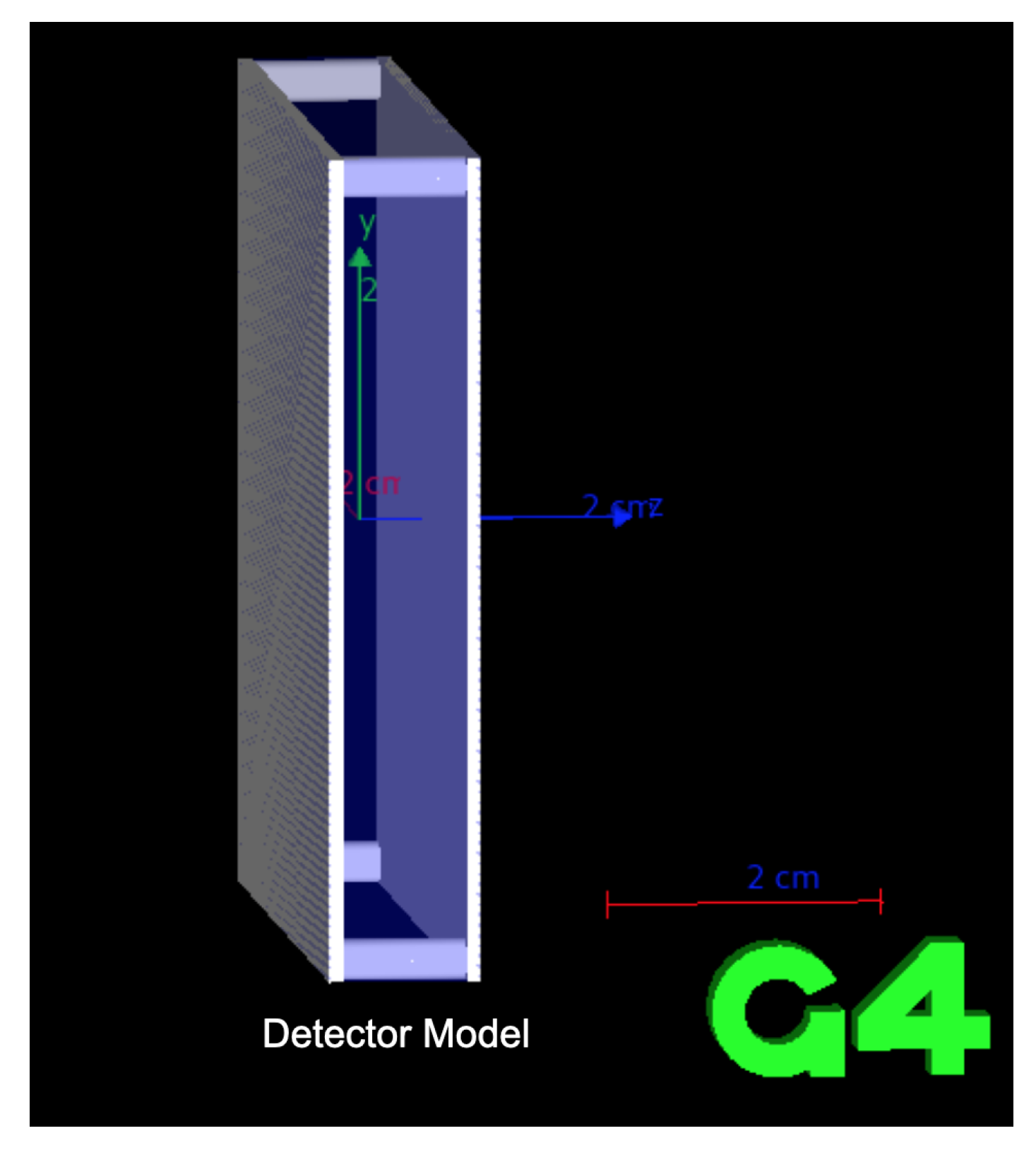
For our simulation, detector geometries identical to those used in the laboratory validation were constructed. Two copper-clad PCB plates with dimensions 5 cm × 5 cm × 1 mm were set in parallel with each other and then placed 1 cm apart. Four cylindrical nylon spacers were placed in the corners of the plates, and an encompassing world volume of air surrounded all of the detector geometries within it. A 3600 V/m electric field was also simulated in the Geant4 program to represent the voltage supplied by batteries in the physical lab. Finally, scoring classes were implemented to count how many secondaries were produced in the world volume, how many reached either plate and deposited charge, and how long the primary particle traveled before decaying or leaving the detector volume. The basic detector geometry as rendered in Geant4 is shown in Figure 1.
The simulations were executed by choosing the primary particle to be detected; in this case, an alpha particle, and then an energy value was assigned to that particle. The particles were then emitted into the detector volume isometrically to represent an alpha source. The simulation then modeled the primary particles interacting with the air molecules by ionization, producing free secondary electrons. The simulated electric field running from plate to plate then interacted with the charged particles by transporting them, using fourth-order Runge–Kutta integration, to either the positive or negatively charged plate, respectively. These charged secondaries were then scored and accumulated into histograms managed by ROOT as a total charge deposited into each plate. To better increase the data collection and performance aspects of the simulation, the program was compiled to run in a multi-threaded configuration where the thread count is 8. This allowed for more efficient execution times of the simulation as well as larger batches of runs, in the range of hundreds of thousands, resulting in more statistically significant data sets.
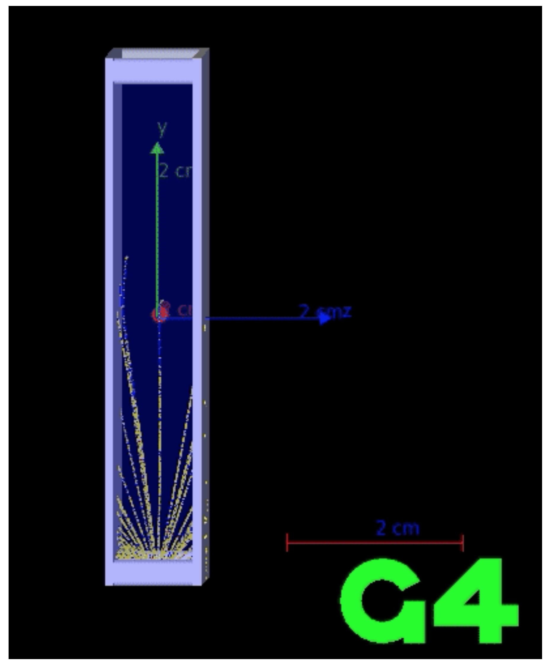
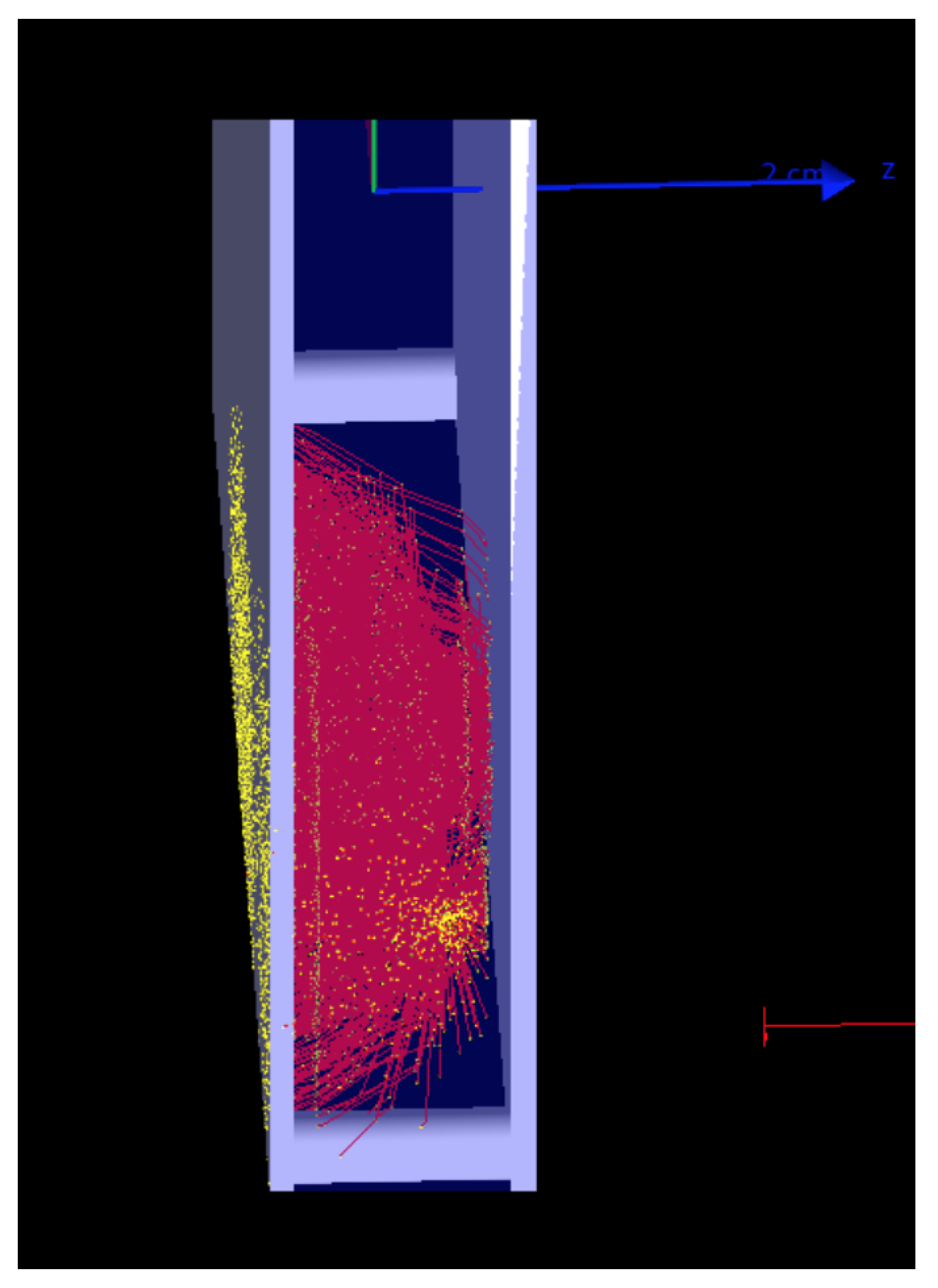
For the simulation involving alpha particles, Geant4 was configured to simulate an Americium-241 source radiating alpha particles in an isotropic distribution with an energy of 5.486 MeV. The alphas then ionized the air between the two plates, the secondary electrons were then scored into the positively charged plate, and the positively charged secondaries were calculated based on the amount of electrons observed. This was performed to simulate the physical lab detector’s expected response to ionization due to an alpha source in the validation measurements described in a later section. The simulated tracks of both the primary alphas and secondary electrons as rendered in Geant4 can be seen in Figure 2, Figure 3, Figure 4, Figure 5 and Figure 6.
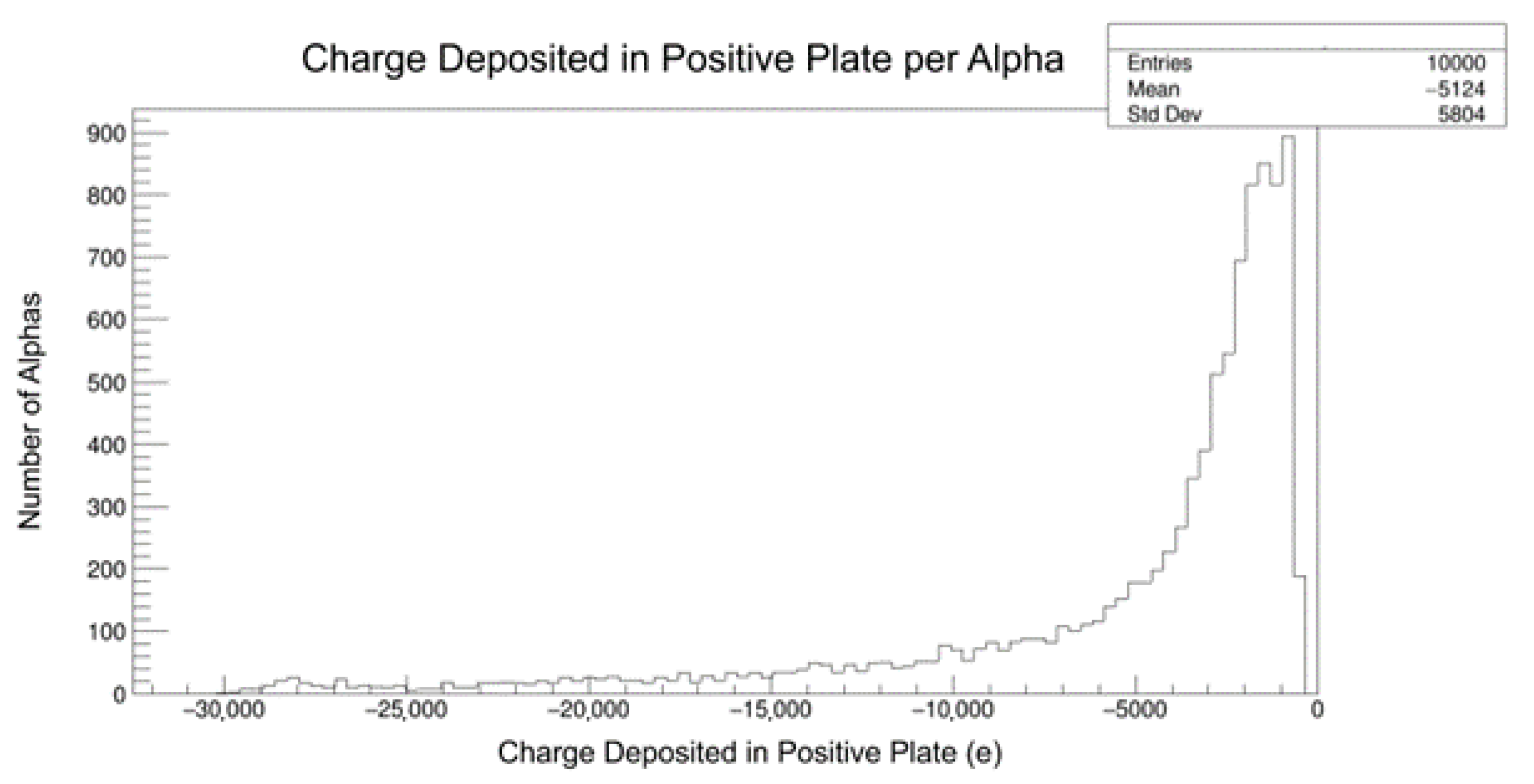
A histogram of the number of simulated alpha events as a function of the number of electrons deposited in the positive plate is shown in Figure 7 for a Geant4 simulation of 10,000 Am-241 alpha decay events. The histogram shows a wide variation in the number of electron charges deposited in the positive plate. This large variation is due primarily to the isotropic nature of the simulated alpha source with the number of secondary electrons produced being strongly dependent on the angle at which the alpha enters the detector. The maximum number of secondary electrons detected corresponds to the case where the alpha is emitted parallel to the plates themselves and travels the full length of the detector interior. The mean of 5124 electrons deposited per alpha in the Geant4 simulation is in good agreement with our measurement of 5020 ± 450 electrons per alpha obtained with the physical detector in the validation described in the following section.
2.3. Experimental Validation with Alpha Particles
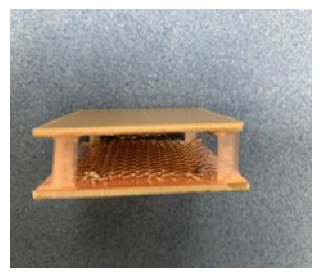
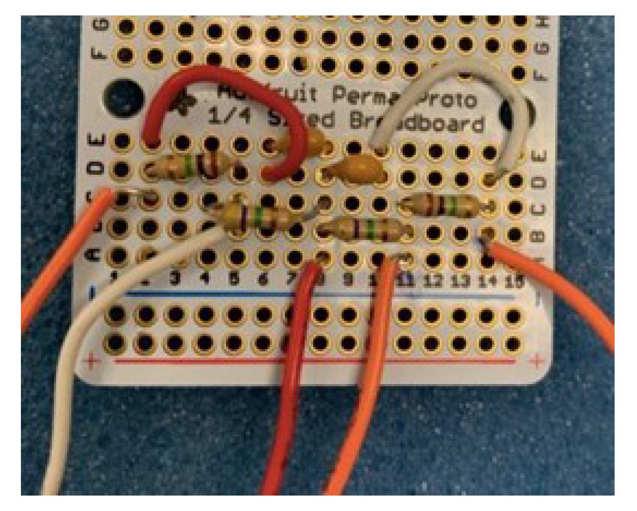
Our alpha simulation was run in parallel with laboratory validation tests on a detector with the same geometry and applied voltage using standard alpha sources [11,12,13]. We constructed detectors that were made of square pieces of copper-clad PCB separated at their corners by nylon spacers to form pairs of parallel plates with the version used for validation having the same dimensions as that in our simulation geometry. A voltage was applied across the plates using a series of four 9-volt batteries and ambient air was used as the gas in the interior. The detectors used in the validation measurements had a 1 cm separation between the plates producing a uniform electric field of 3600 V/m in the detector interior. Any ionization current produced by charged particles passing through the air in the detector interior was collected on the plates and passed through a large resistor and the voltage across the resistor was read out by a nanovoltmeter. Examples of the physical detectors may be seen in Figure 8, Figure 9 and Figure 10. The operating principle of the detectors was similar to that used in a standard ionizing smoke detector [14].
To validate the simulation’s prediction of the ability of the parallel-plate detectors to observe ionization currents, 0.9 Curie alpha-emitting Am-241 sources were placed at the edge of the detector midway between the parallel plates. A constant electric field of 3600 V/m was applied between the plates. For each trial of the detector, 0, 1, 2, 3, and 4 sources were placed the at center of the detector edge, and the resulting ionization current was recorded. In order to minimize statistical errors the ionization current measurements were made with 150 trials per source. In running multiple trials, Lab View was used to collect repeated voltage readings from the nanovoltmeter with the time between each reading being fixed. The mean voltage for each trial with a specific number of sources was used as the voltage for that data point and the standard deviation of the set of readings for that data point was used as the statistical error. A set of trails was conducted using both 15 M of resistance and 20 M of resistance between the plates. The results were then plotted for multiple trials using the voltage differences between the reading on the nanovoltmeter with the specific number of sources present and the reading on the nanovoltmeter with no sources present.
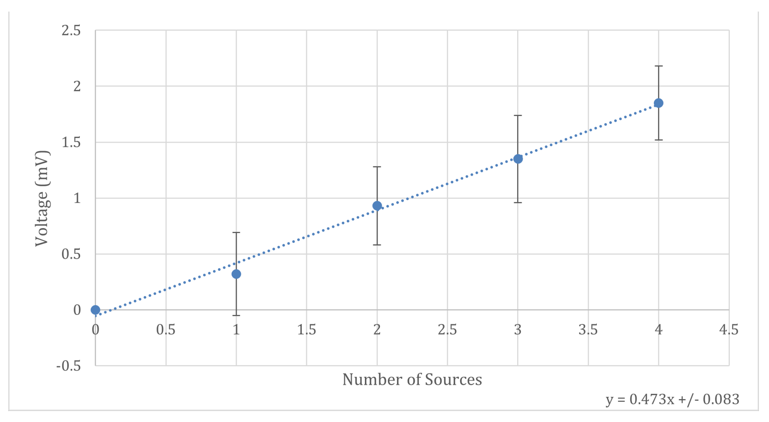
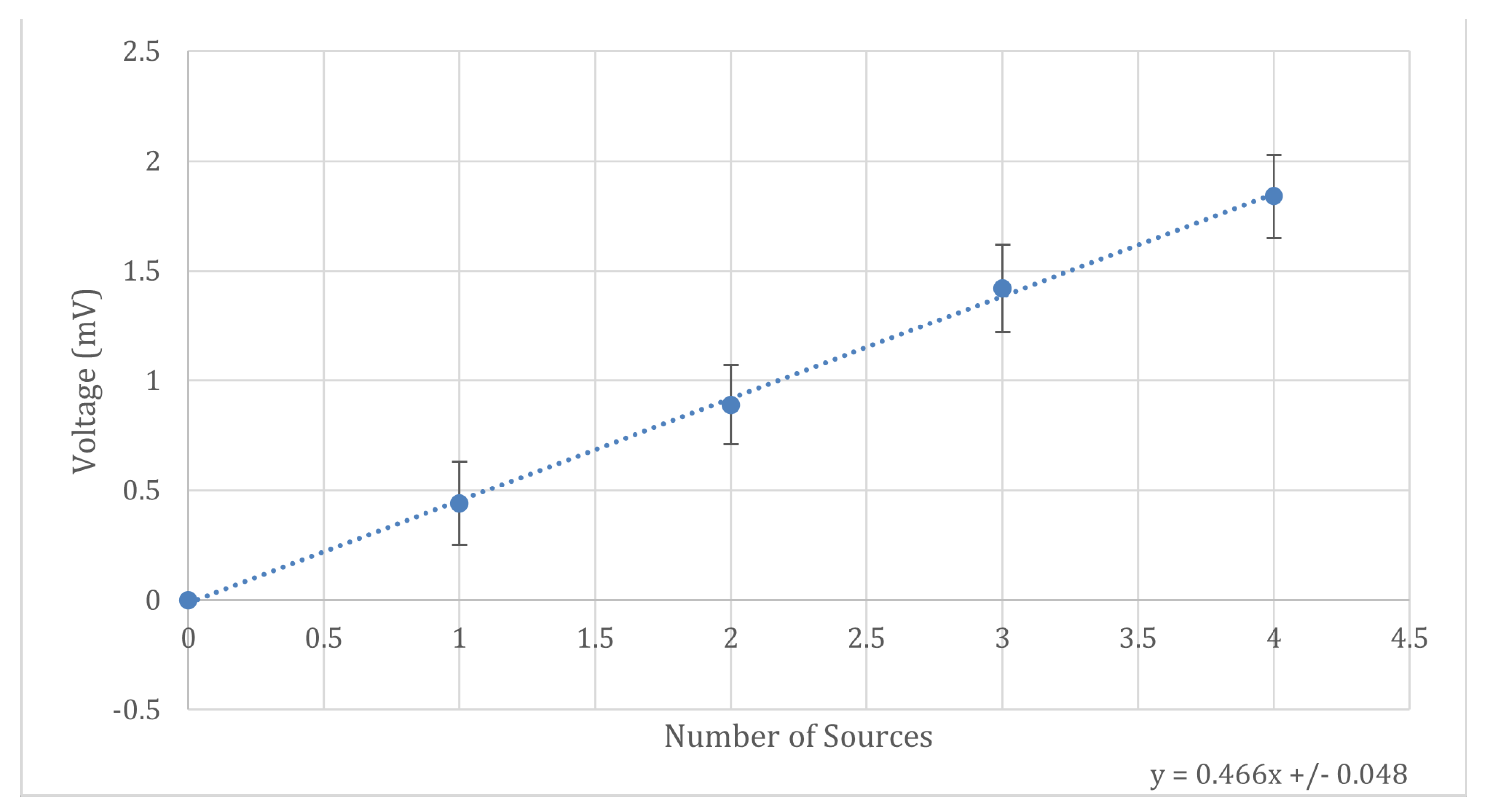
The slope of the plot for the 15 M resistor in millivolts per source is 0.473 ± 0.083, as shown in Figure 11. To determine the number of electrons deposited in the positive plate for each alpha particle, the slope of the graph in millivolts per source was converted to secondaries per alpha. For the 15 M resistor this corresponded to a current of 31.5 pA per alpha source. As each alpha source has a strength of 0.9 microCuries this corresponded to 6420 ± 1130 electrons detected per alpha. The slope of the plot for the 20 M resistor in millivolts per source is 0.466 ± 0.048 as shown in Figure 12. To determine the number of electrons deposited in the positive plate for each alpha particle, the slope of the graph in millivolts per source was converted to secondaries per alpha. For the 20 M resistor, this corresponded to a current of 23.3 pA per alpha source which corresponded to 4750 ± 490 electrons detected per emitted alpha.
A total of 150 trials were run for the 15 MOhm circuit, and another 150 trials were run with the 20 MOhm circuit for a total of 300 measurement trials. For all 300 trials for both circuits, the weighted mean of the number of electrons detected per alpha emitted was found to be 5020 ± 450, which is consistent with the mean value of 5124 electrons per alpha found in the simulation.
2.4. Geant4 Modeling of Detector with Muons
Once the Geant4 simulation geometry had been validated for alpha sources, the incoming particles were modified in the code to simulate the detector’s response to cosmic ray muons as the primary source. In general, alphas and muons have different physics properties, but both are charged and capable of ionizing air molecules creating secondary electrons that may be deposited in the detector. One important difference is that while alphas deposit the majority of their energies in the volume of the detector, muons are much more penetrating and mostly traverse the detector volume. Only in a very specific energy range do the muons ionize an appreciable amount of air in the first few centimeters. For this reason, the small detectors have such a specific energy range for detection, and this range can be seen via simulation.
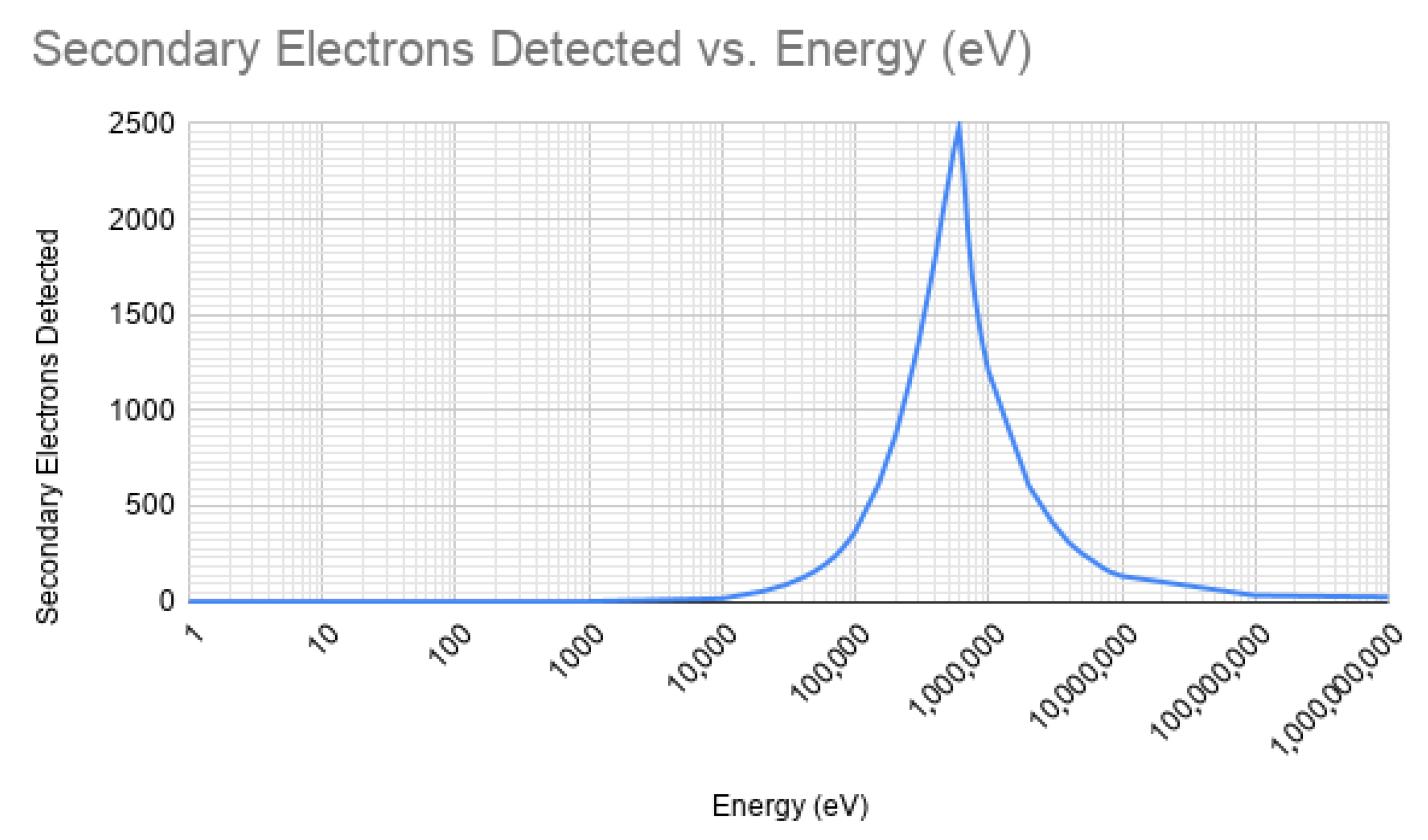
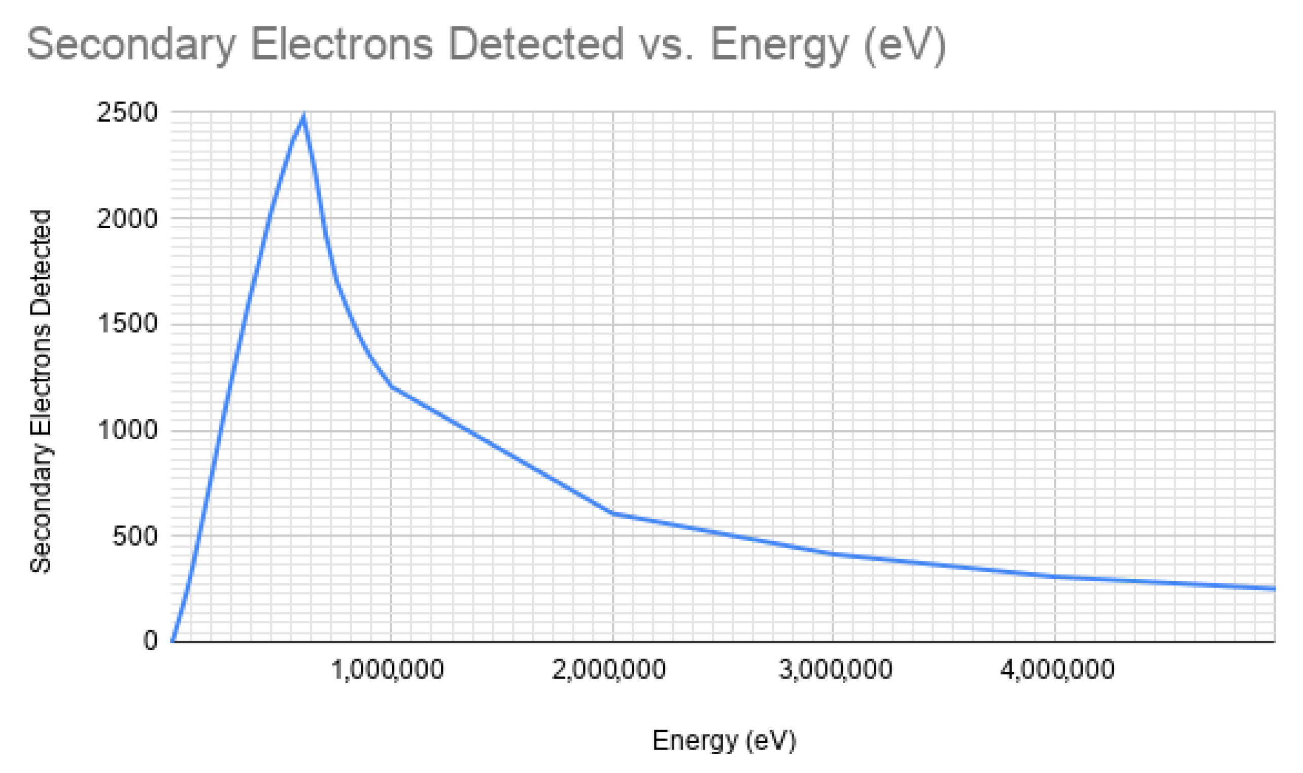
For simulations in which muon was the incoming particle, Geant4 was run in particle gun mode to simulate cosmic ray muons originating from above. For this simulation, the muons were given initial kinetic energies ranging from 1 eV to 1 GeV and were passed through the entire length of the detector (5.0 cm) in order to see the maximum possible current detected. The response of the detector was highly energy dependent with the greatest ionization current observed for muons with vertical trajectories in an energy range centered around 600 keV of kinetic energy. For these muons, an average of 2479 secondary electrons were produced in Geant4 for every muon passing through the entire volume of the detector. For muons below this energy range, insufficient energy was available to ionize the air molecules and lead to electrons being deposited on the plates. For muons above this energy range, very few ionizations were found to be produced and the muon instead traversed the entire detector without depositing an appreciable amount of its energy through ionization. The number of secondary electrons produced in Geant4 as a function of muon kinetic energy can be seen in Figure 13 and Figure 14.
Once the simulation had been tested on the basic detector geometry, layers of concrete were added between the particle source and detector to investigate the effects of the material on the energies of the muons and the subsequent change in the number of secondary electrons and ionization currents seen in the simulated detector. For the portion of the simulation that involved large-statistics Geant4 runs including material, the entire simulation was moved from a desktop to a Linux cluster as described in the following section.
2.5. Computing Environments for Muon Simulations
The Geant4 simulations were run initially on a desktop environment with CentOS, a Linux distribution, as the OS. The desktop’s quad-core Intel processor and 16 GB of ram proved useful for tuning the simulations, but because of the time required to run a large statistics simulation, it was apparent that a more powerful system would be necessary for that case. For our large-scale muon simulation, Geant4 was configured to run on a cluster of 12 servers. This cluster contained 96 CPU cores and could provide over two orders of magnitude greater statistics. The components of the cluster included 10 PowerEdge R410 dual quad-core processors for use as worker nodes of the system (each with 2 × 250 GB of hard drive storage), 2 PowerEdge R710 dual quad-core processors for use as an NFS gatekeeper and an interactive testing node (each with 2 × 250 GB of hard drive storage), and a PowerVault MD1200 rack mount with 12 1 TB 7.2 K RPM hard drives, for a total storage of 18 TB. Configuring the cluster to run a large statistics Geant4 simulation required setting up identical environments across all nodes via a CentOS command-line shell.
2.6. Muon Simulation Parameters
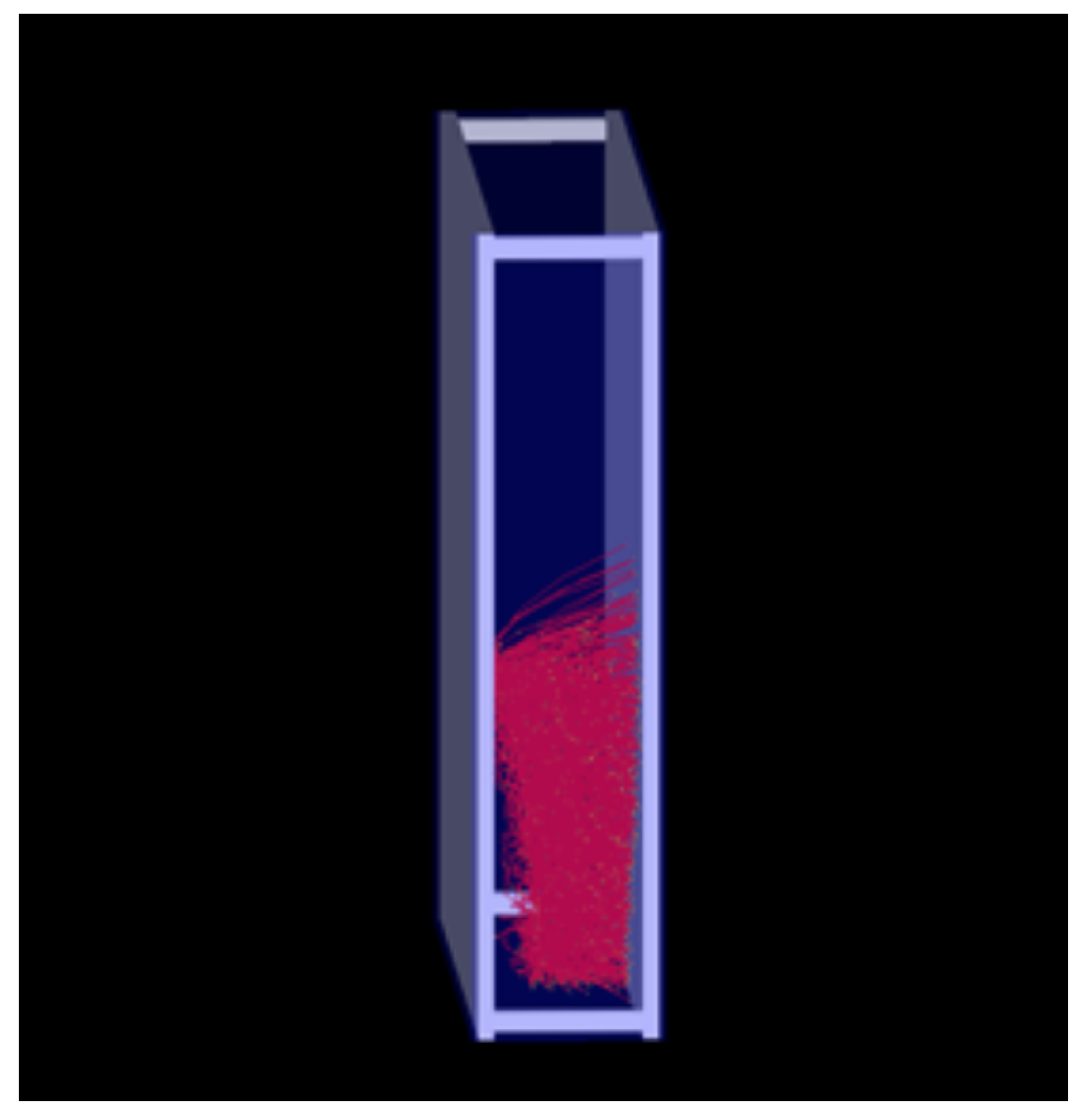
For the large-statistics simulations, seven different geometries were run, each one having a layer of concrete of a specific thickness (0.1 cm, 0.2 cm, 0.3 cm, 0.4 cm, 0.5 cm, 1.0 cm, and 2.0 cm) situated between the muon source and the detector. Each simulation consisted of 10,000 muons per event and an event at every 1000 eV step from 4,000,000 eV to 50,000,000 eV. The total size of the simulation for all seven thicknesses of the concrete layer across all muon energies was 3,220,000,000 total muons simulated and recorded. The secondary tracks produced by a single muon in the large-scale simulation run as rendered in Geant4 are shown in Figure 15.
3. Results
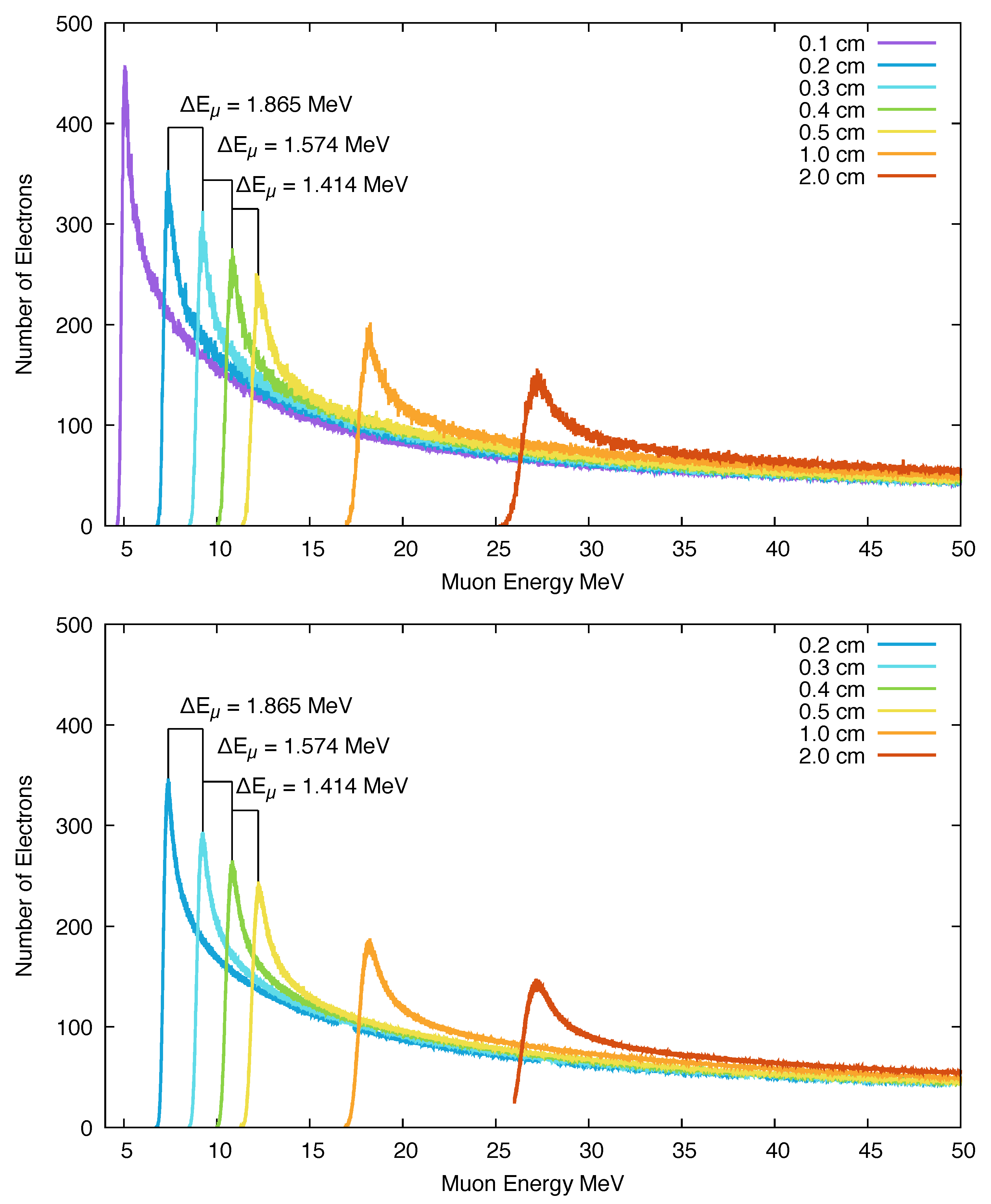
The large-scale simulation was run in two stages. The first stage consisting of 6 million events was run to ensure that the job-management system on the cluster was working properly and that the results from the simulation run on the cluster nodes were consistent with those run in the desktop environment. The second stage consisted of 3.22 billion events and was run over a period of several months. For each muon in each run, the number of secondary electrons produced in the simulation was recorded and plotted for each of the seven thicknesses of concrete as a function of the initial muon kinetic energy. The random number seed was set when the simulation was initialized for the first event of each run and not reinitialized until the run was completed in order that no two muons in a single run would produce identical outputs. Once the run was completed, the input parameters (i.e., the initial energy) were changed; the maximum number of muons generated with identical input parameters was 10,000. The results of the first and second stages of the simulation are shown in Figure 16. In this figure, the top plot shows the number of secondary electrons detected per muon for each run of 1000 muons which were generated for every 10 keV of initial energy. The bottom plot shows the number of secondary electrons detected per muon for each run of 10,000 muons, which were generated for every 1 keV of initial energy.
These figures summarize the results from the simulation runs on the cluster and the effect of the larger statistics can be seen by comparing the smoothness of the curves between Figure 16 top and bottom. In these graphs, the y-axis represents the total number of secondary electrons detected by the detector while the x-axis represents the muon’s initial kinetic energy. The seven different colored lines plotted in the graphs are the simulations run with varying concrete thicknesses. The primary trend shown by the graph is that as the thickness of the material is increased, the incoming muon requires a higher initial kinetic energy to penetrate the material and be detected, resulting in a measurable change in the energy of the peak response of the detector.
Comparing the case of the 0.2 cm and 0.3 cm concrete layer thicknesses, the initial muon kinetic energy, which corresponds to peak secondary electron production in the detector, increases by a value of 1.865 MeV. For the case of the 0.3 and 0.4 cm layer thicknesses, this difference is found to be 1.574 MeV, and for the case of the 0.4 and 0.5 cm layer thicknesses, the difference is found to be 1.414 MeV. These values are compared to the expected results from the literature in the following discussion section.
4. Discussion
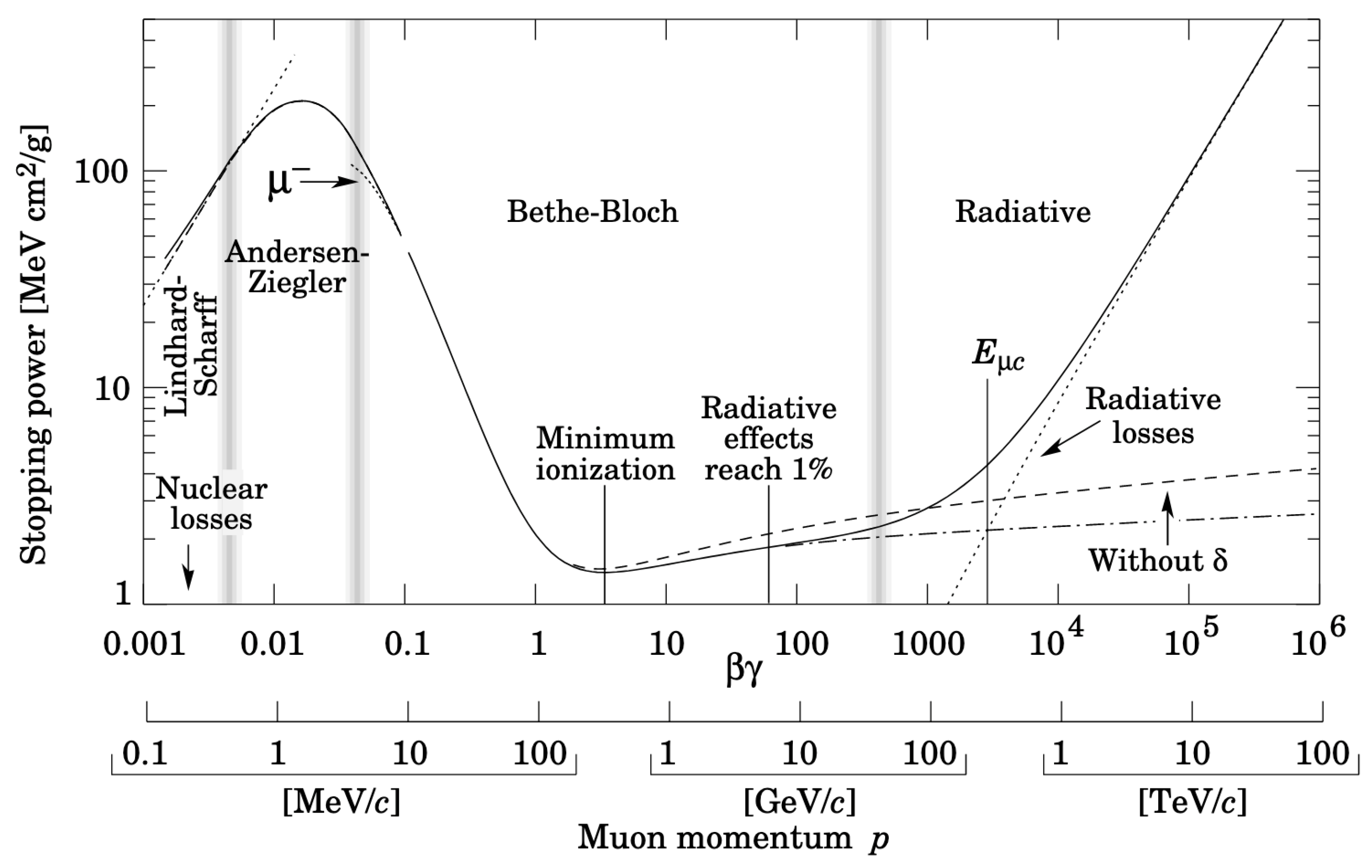
In order to make a comparison between the results of our Geant4 simulation and the expected loss in muon energy from the literature, we used the report from Groom et al. entitled “Muon Stopping Power and Range Tables 10 MeV–100 TeV” published in Atomic and Nuclear Data Tables in 2001 [15]. Figure 17 shows one of the plots from that reference which illustrates the muon stopping power as a function of momentum and . The muons that produce a peak signal in our detectors fall in the lower momentum portion of the Bethe-Block region shown in Figure 17. As this region has a falling slope in terms of stopping power vs. muon momentum we expect smaller amounts of energy loss per millimeter of concrete as the thickness is increased, which is consistent with the results shown in Figure 16.
Comparing the graphs from our simulations to the graphs from Groom et al. [15], we can cross-check the accuracy of the results from Geant4. For the muons traversing 0.2 cm of concrete, we find a peak signal in our detector at 7.0 MeV of initial muon kinetic energy. This energy corresponds to a of 1.066 and a of 0.346 for a combined of 0.369. This corresponds in Groom et al. to a muon momentum with an expected stopping power of 8 MeV cm/g, as can be seen in Figure 17. Given a concrete density in our Geant4 simulation of 2.3 g/cm, this gives an energy loss of 1.84 MeV/mm, which is in good agreement with the energy difference between our 0.2 cm and 0.3 cm concrete layers of 1.865 MeV.
For the muons traversing the 0.3 cm concrete layer, we find a peak detector signal in our simulation for incoming kinetic energies of 8.9 MeV. This energy corresponds to a of 1.084 and a of 0.386 for a combined of 0.418. For this , the reference gives a stopping power of 6.5 MeV cm/g corresponding to an energy difference between the 0.3 and 0.4 cm layers of 1.495 MeV/mm, as compared to 1.574 MeV/mm from our simulation. As the layers become thicker this simple comparison becomes less appropriate due to the effect of the changing stopping power over the course of the muon traversing the concrete. For the energy corresponding to the peak detector signal of 0.4 cm, for example, we find an incoming kinetic energy of peak detection of 10.4 MeV, corresponding to a of 0.455. For this value, the reference gives a stopping power of 5 MeV cm/g corresponding to an energy difference between the 0.4 cm and 0.5 cm layers of 1.15 MeV/mm as compared to 1.414 MeV/mm from our simulation. We conclude that for concrete layers with thicknesses above 3–4 mm a single value cannot be accurately assigned to the muon stopping power. The basic reason for this is that the muons at these energies are in the falling stopping power portion of the Bethe-Bloch region below the point of minimum ionization as seen in Figure 17. In this region, the stopping power decreases rapidly as the muons deposit energy in the material, and the Geant4 simulation is preferable for a detailed analysis of energy loss rather than the use of a single value for the stopping power. In our figures, we have included the results for 1 cm and 2 cm layers of concrete in our simulation to illustrate the effects of thicker concrete layers on the muon energy, including the broadening of the peak detection energy curve.
Running our simulation at very high statistics (3.2 billion events) did not appreciably change the results from the simulation run with 6 million events for the thin concrete layers we modeled. In particular, the energies of peak detection remained the same to within 1 keV even with 500 times the number of events run, and we conclude that extremely high statistics runs are not needed for this type of analysis, although they may be useful in more complicated scenarios.
Author Contributions
Conceptualization, D.J.; Methodology, D.J. and C.P.; Software, C.P.; Validation, D.J. and C.P.; Formal analysis, D.J.; Investigation, D.J. and C.P.; Resources, D.J.; Data curation, C.P.; Writing—original draft, D.J.; Writing—review & editing, C.P.; Visualization, C.P.; Supervision, D.J.; Project administration, D.J.; Funding acquisition, D.J. All authors have read and agreed to the published version of the manuscript.
Funding
This research was funded by the Birla Carbon Scholars Program at Kennesaw State University and the Georgia Space Grant Consortium (Awards AP645486 and AP313425).
Data Availability Statement
The data presented in this study are available on request from the corresponding author.
Acknowledgments
The authors would like to acknowledge the support of the Kennesaw State University Department of Physics and the following individuals: Ryan Beckett, Katie Bishop, Gracyn Jewett, Michael Reynolds, Emma Pearson, and Kevin Stokes.
Conflicts of Interest
The authors declare no conflict of interest. The funders had no role in the design of the study; in the collection, analyses, or interpretation of data; in the writing of the manuscript; or in the decision to publish the results.
References
- Oláh, L.; Barnaföldi, G.G.; Hamar, G.; Melegh, H.G.; Surányi, G.; Varga, D. Cosmic Muon Detection for Geophysical Applications. Adv. High Energy Phys. 2013, 2013, 560192. [Google Scholar] [CrossRef]
- Bonechi, L.; D’Alessandro, R.; Giammanco, A. Atmospheric Muons as an Imaging Tool. Rev. Phys. 2020, 5, 100038. [Google Scholar] [CrossRef]
- Tioukov, V.; Alexandrov, A.; Bozza, C.; Consiglio, L.; D’Ambrosio, N.; De Lellis, G.; De Sio, C.; Giudicepietro, F.; Macedonio, G.; Miyamoto, S.; et al. First Muography of Stromboli Volcano. Sci. Rep. 2019, 9, 6695. [Google Scholar] [CrossRef] [PubMed]
- Saracino, G.; Carloganu, C. Looking at Volcanoes with Cosmic Ray Muons. Phys. Today 2012, 65, 60–61. [Google Scholar] [CrossRef]
- Cimmino, L.; Baccani, G.; Noli, P.; Amato, L.; Ambrosino, F.; Bonechi, L.; Bongi, M.; Ciulli, V.; D’Alessandro, R.; D’Errico, M.; et al. 3D Muography for the Search of Hidden Cavities. Sci. Rep. 2019, 9, 2974. [Google Scholar] [CrossRef] [PubMed]
- Nappi, E.; Peskov, V. Imaging Gaseous Detectors and Their Applications; WileyVCH: Weinheim, Germany, 2013. [Google Scholar]
- Agostinelli, S.; Allison, J.; Amako, K.A.; Apostolakis, J.; Araujo, H.; Arce, P.; Asai, M.; Axen, D.; Banerjee, S.; Barrand, G.J.N.I. Geant4—A Simulation Toolkit. Nucl. Instrum. Methods Phys. Res. Sect. A 2013, 506, 250–303. [Google Scholar] [CrossRef]
- Allison, J.; Amako, K.; Apostolakis, J.E.; Araujo, H.A.; Dubois, P.A.; Asai, M.A.; Barr, G.A.; Capra, R.A.; Chauvie, S.A.; Chytracek, R.A. Geant4 Developments and Applications. IEEE Trans. Nucl. Sci. 2006, 53, 270–278. [Google Scholar] [CrossRef]
- Allison, J.; Amako, K.; Apostolakis, J.; Arce, P.; Asai, M.; Aso, T.; Bagli, E.; Bagulya, A.; Banerjee, S.; Barr, G.J. Recent Developments in Geant4. Nucl. Instrum. Methods Phys. Res. Sect. A 2016, 835, 186–225. [Google Scholar] [CrossRef]
- Geant4 Book for Application Developers. Available online: https://geant4-userdoc.web.cern.ch (accessed on 12 May 2023).
- Bishop, K.; Joffe, D. Design, Development and Testing of a Parallel Plate Particle Detector. In Proceedings of the National Council on Undergraduate Research Annual Meeting, Virtual, 12–14 April 2021. [Google Scholar]
- Jewett, G.; Joffe, D. Readout Electronics for a Multi Wire Proportional Chamber. In Proceedings of the National Council on Undergraduate Research Annual Meeting, Virtual, 12–14 April 2021. [Google Scholar]
- Jewett, G.; Joffe, D. Simulation of an AD8099 Operational Amplifier for Use in the Readout Electronics of a Muon Detector. Kennesaw J. Undergrad. Res. 2021, 8, 2. [Google Scholar]
- Rork, G.; Schlachter, A.; Simon, F.; Stryk, R. Ionization Smoke Detector. U.S. Patent 3,735,138, 22 May 1973. [Google Scholar]
- Groom, D.E.; Mokhov, N.V.; Striganov, S.I. Muon stopping-power and range tables: 10 MeV–100 TeV. At. Data Nucl. Data Tables 2001, 78, 183–356. [Google Scholar] [CrossRef]
Figure 1.
The detector geometry constructed in GEANT4.

Figure 2.
Primary tracks from 100 simulated alpha particles traveling through the detector volume from the source located at the center of a detector edge.
Figure 2.
Primary tracks from 100 simulated alpha particles traveling through the detector volume from the source located at the center of a detector edge.

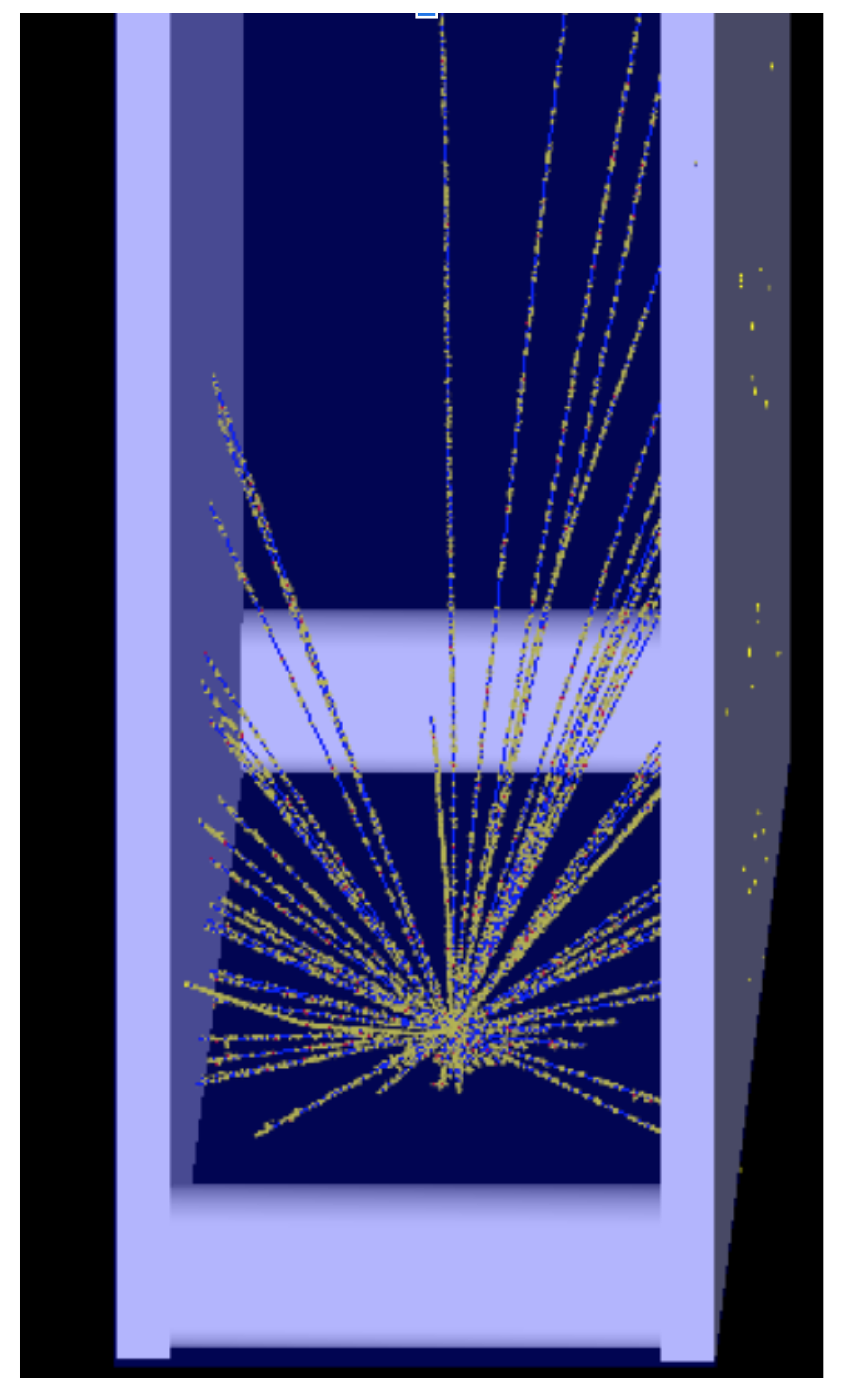
Figure 3.
Close-up of primary tracks from simulated alpha particles traveling through the detector volume.
Figure 3.
Close-up of primary tracks from simulated alpha particles traveling through the detector volume.

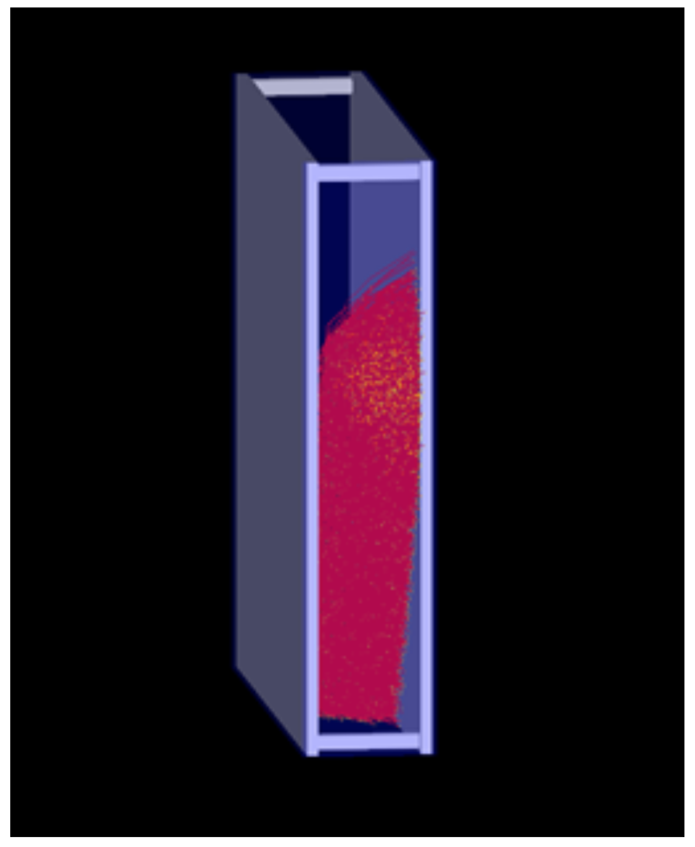
Figure 4.
Secondary electron tracks from a single simulated alpha particle traversing the air in the interior of the detector and producing electrons via ionization. The effects of the electric field on the secondary electrons are visible.
Figure 4.
Secondary electron tracks from a single simulated alpha particle traversing the air in the interior of the detector and producing electrons via ionization. The effects of the electric field on the secondary electrons are visible.

Figure 5.
Close-up of secondary electron tracks produced from simulated alpha particles ionizing the air in the volume of the detector.
Figure 5.
Close-up of secondary electron tracks produced from simulated alpha particles ionizing the air in the volume of the detector.

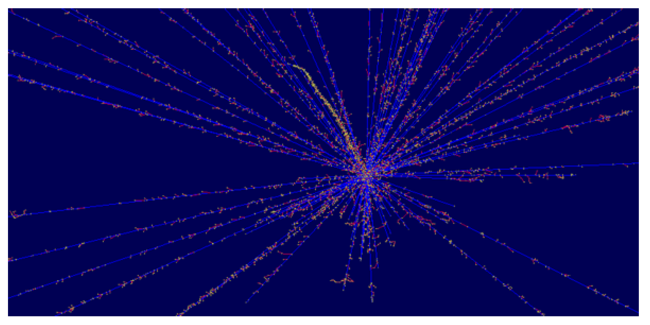
Figure 6.
Close-up view of simulated primary and secondary tracks produced in Geant4 for alpha sources in air in the absence of a detector.
Figure 6.
Close-up view of simulated primary and secondary tracks produced in Geant4 for alpha sources in air in the absence of a detector.

Figure 7.
Simulated electron charge deposited in the positive plate for alpha particles. The deposited charge is scored in Geant4 as a negative value in units of the electronic charge.
Figure 7.
Simulated electron charge deposited in the positive plate for alpha particles. The deposited charge is scored in Geant4 as a negative value in units of the electronic charge.

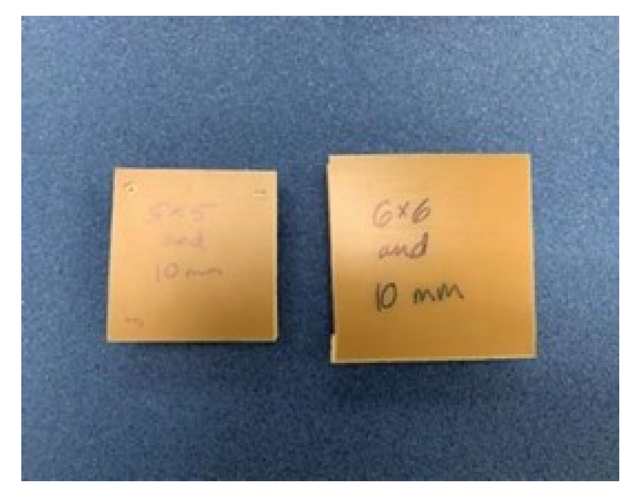
Figure 8.
Sample detectors of different sizes. A detector size of 5 cm × 5 cm × 1 cm was used in the final version for both the laboratory tests and the Geant4 simulation.
Figure 8.
Sample detectors of different sizes. A detector size of 5 cm × 5 cm × 1 cm was used in the final version for both the laboratory tests and the Geant4 simulation.

Figure 9.
Side view of a sample detector with a wire mesh added to the interior. The mesh was removed in the final version used in both the laboratory tests and the Geant4 simulation.
Figure 9.
Side view of a sample detector with a wire mesh added to the interior. The mesh was removed in the final version used in both the laboratory tests and the Geant4 simulation.

Figure 10.
Resistors used for readout of the ionization current produced between the plates.

Figure 11.
Voltage difference as a function of the number of sources for the 15 M resistor.

Figure 12.
Voltage difference as a function of the number of sources for the 20 M resistor.

Figure 13.
Number of secondary electrons produced in simulation as a function of energy (logarithmic energy scale).
Figure 13.
Number of secondary electrons produced in simulation as a function of energy (logarithmic energy scale).

Figure 14.
Number of secondary electrons produced in simulation as a function of energy (linear energy scale).
Figure 14.
Number of secondary electrons produced in simulation as a function of energy (linear energy scale).

Figure 15.
Geant4 simulation of a single muon traversing the space in the detector including the production of secondary electrons. The effects of the electric field on the secondary electrons are visible as the asymmetry in the trajectories of the secondary tracks.
Figure 15.
Geant4 simulation of a single muon traversing the space in the detector including the production of secondary electrons. The effects of the electric field on the secondary electrons are visible as the asymmetry in the trajectories of the secondary tracks.

Figure 16.
Results from the first stage (top) and second stage (bottom) of the simulation for 6 million muons and 3.22 billion muons, respectively, and the corresponding simulated secondary electrons deposited in the detector plates. The geometry for the 0.1 cm concrete thickness was not run in the higher statistics simulation.

Figure 17.
Muon stopping power as a function of muon momentum [15].
Figure 17.
Muon stopping power as a function of muon momentum [15].

Disclaimer/Publisher’s Note: The statements, opinions and data contained in all publications are solely those of the individual author(s) and contributor(s) and not of MDPI and/or the editor(s). MDPI and/or the editor(s) disclaim responsibility for any injury to people or property resulting from any ideas, methods, instructions or products referred to in the content. |
© 2023 by the authors. Licensee MDPI, Basel, Switzerland. This article is an open access article distributed under the terms and conditions of the Creative Commons Attribution (CC BY) license (https://creativecommons.org/licenses/by/4.0/).
Share and Cite
MDPI and ACS Style
Joffe, D.; Perez, C. Geant4 Simulation of Muon Absorption in Concrete Layers. Instruments 2023, 7, 17. https://doi.org/10.3390/instruments7020017
AMA Style
Joffe D, Perez C. Geant4 Simulation of Muon Absorption in Concrete Layers. Instruments. 2023; 7(2):17. https://doi.org/10.3390/instruments7020017
Chicago/Turabian StyleJoffe, David, and Christian Perez. 2023. "Geant4 Simulation of Muon Absorption in Concrete Layers" Instruments 7, no. 2: 17. https://doi.org/10.3390/instruments7020017