Article

Innovative Analytical Method for X-ray Imaging and Space-Resolved Spectroscopy of ECR Plasmas

1
Laboratori Nazionali del Sud, Istituto Nazionale di Fisica Nucleare, Via S. Sofia 62, 95123 Catania, Italy
2
Institute for Nuclear Research (Atomki), Bem Square 18/c, 4026 Debrecen, Hungary
3
Laboratori Nazionali di Legnaro, Istituto Nazionale di Fisica Nucleare, Viale dell’Università 2, 35020 Legnaro, Italy
*
Author to whom correspondence should be addressed.
Condens. Matter 2022, 7(1), 5; https://doi.org/10.3390/condmat7010005
Submission received: 24 October 2021 / Revised: 16 November 2021 / Accepted: 24 November 2021 / Published: 28 December 2021
(This article belongs to the Special Issue High Precision X-ray Measurements 2021)

Abstract

:
At the Italian National Institute for Nuclear Physics-Southern National Laboratory (INFN-LNS), and in collaboration with the ATOMKI laboratories, an innovative multi-diagnostic system with advanced analytical methods has been designed and implemented. This is based on several detectors and techniques (Optical Emission Spectroscopy, RF systems, interfero-polarimetry, X-ray detectors), and here we focus on high-resolution, spatially resolved X-ray spectroscopy, performed by means of a X-ray pin-hole camera setup operating in the 0.5–20 keV energy domain. The diagnostic system was installed at a 14 GHz Electron Cyclotron Resonance (ECR) ion source (ATOMKI, Debrecen), enabling high-precision, X-ray, spectrally resolved imaging of ECR plasmas heated by hundreds of Watts. The achieved spatial and energy resolutions were 0.5 mm and 300 eV at 8 keV, respectively. Here, we present the innovative analysis algorithm that we properly developed to obtain Single Photon-Counted (SPhC) images providing the local plasma-emitted spectrum in a High-Dynamic-Range (HDR) mode, by distinguishing fluorescence lines of the materials of the plasma chamber (Ti, Ta) from plasma (Ar). This method allows for a quantitative characterization of warm electrons population in the plasma (and its 2D distribution), which are the most important for ionization, and to estimate local plasma density and spectral temperatures. The developed post-processing analysis is also able to remove the readout noise that is often observable at very low exposure times (msec). The setup is now being updated, including fast shutters and trigger systems to allow simultaneous space and time-resolved plasma spectroscopy during transients, stable and turbulent regimes.

1. Introduction

At the Italian National Institute for Nuclear Physics—Southern National Laboratory (INFN-LNS) and in collaboration with the ATOMKI Laboratories, efforts have been devoted to the study, development and use of an innovative multi-diagnostic setup with advanced analytical techniques aiming to characterize the thermodynamical properties of the Electron Cyclotron Resonance (ECR)-magnetized plasmas confined in compact traps for multidisciplinary studies. The developed multi-diagnostics setup [1,2] includes a microwave interfero-polarimeter, several RF multi-pin probes, a multi-X-ray detector system for X-ray spectroscopy, a X-ray pin-hole camera for high-resolution, 2D, space-resolved spectroscopy and different spectrometers for plasma-emitted visible-light characterization.
In the framework of the Plasmas for Astrophysics, Nuclear Decays Observation and Radiation for Archaeometry (PANDORA) project [3], the multi-diagnostic system will equip an innovative compact and flexible magnetic plasma trap to measure the nuclear β -decay rates of nuclear astrophysics interest, for the first time, in laboratory plasmas [4]. On the other hand, plasma diagnostics plays a crucial role in some applications, i.e., for the development and the improvement of future ECR ion sources (ECRISs) that can produce beams of highly charged ions with the high intensity and stability that are necessary for accelerators in applied and nuclear physics research.
Among other techniques, X-ray plasma diagnostics have been developed over the years, allowing for the volumetric characterization of ECR plasmas [5,6,7,8,9]. The volume-integrated X-ray diagnostics in the soft-X domain (from 1 keV to 30 keV) allow us to probe the “warm” plasma population, which plays a crucial role in ionization and charge distribution build-up. Several experimental campaigns have been carried out at INFN-LNS, at the GSI-Darmstadt and at ATOMKI-Debrecen [10,11,12], measuring the temperature and density of warm electrons by applying an emissivity model [13].
High-precision X-ray measurements can be also performed in a spatially resolved way by means of the powerful X-ray pin-hole camera tool, which allows us to perform high-resolution, spatially resolved spectroscopy. Even if our teams have already been using the X-ray camera techniques combined with pinholes for more than 15 years [14,15,16,17,18,19], and this method has been routinely used in several other laboratories (for example, at Z-machines [20,21,22,23] or in plasma fusion devices [24,25,26,27]), recently, both the tool [28] and the advanced analytical method have been drastically improved.
In this paper, a developed analytical method is presented. A suite of MatLab codes has been developed from the ground-up, supporting the analysis of the X-ray pin-hole camera raw images. The algorithm is now able to analyze the Single Photon-Counting (SPhC) images for energy-resolved investigation pixel-by-pixel to investigate the local plasma-emitted spectrum in a High-Dynamic-Range (HDR) mode by distinguishing the fluorescence lines of the materials of the plasma chamber (Ti, Ta) from plasma (Ar) fluorescence lines; moreover, a very high energy and spatial resolution has been achieved (respectively of 300 eV at 8.1 keV and 500 μ m) by means of a part of the developed code that is able to remove the readout noise that typically affects measurements acquired with very low exposure times t e x p (several tens of milliseconds), such as the ones taken in SPhC mode, almost completely. As a consequence, this method allows for quantitative characterization of the population of warm electrons in the plasma (and its 2D distribution), an estimation of the local plasma density and spectral temperatures and an investigation of the plasma morphology and confinement dynamics in an ECR plasma trap. The analytical method and tool can also be useful in other devices, i.e., for plasma fusion or applications.

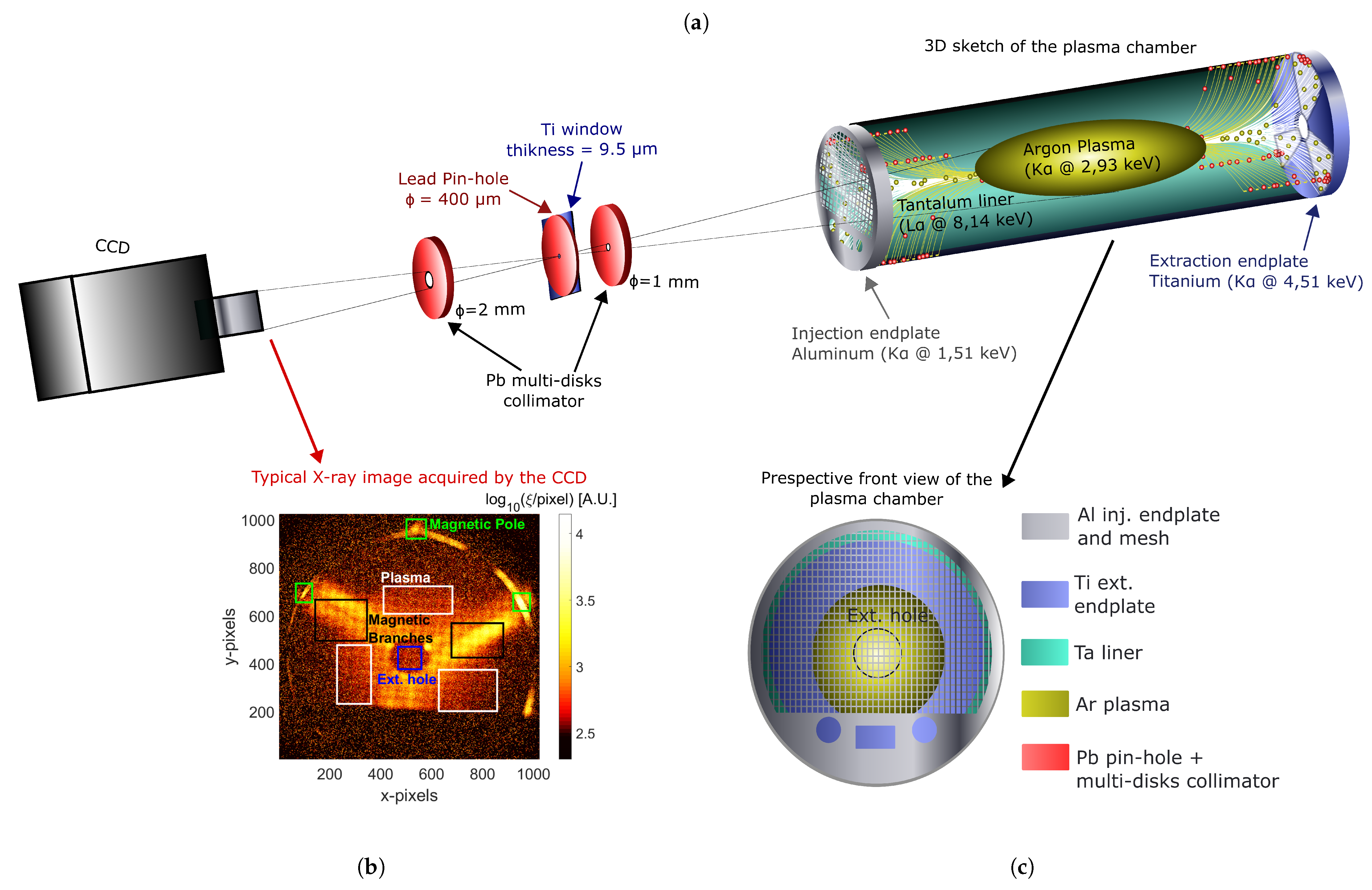
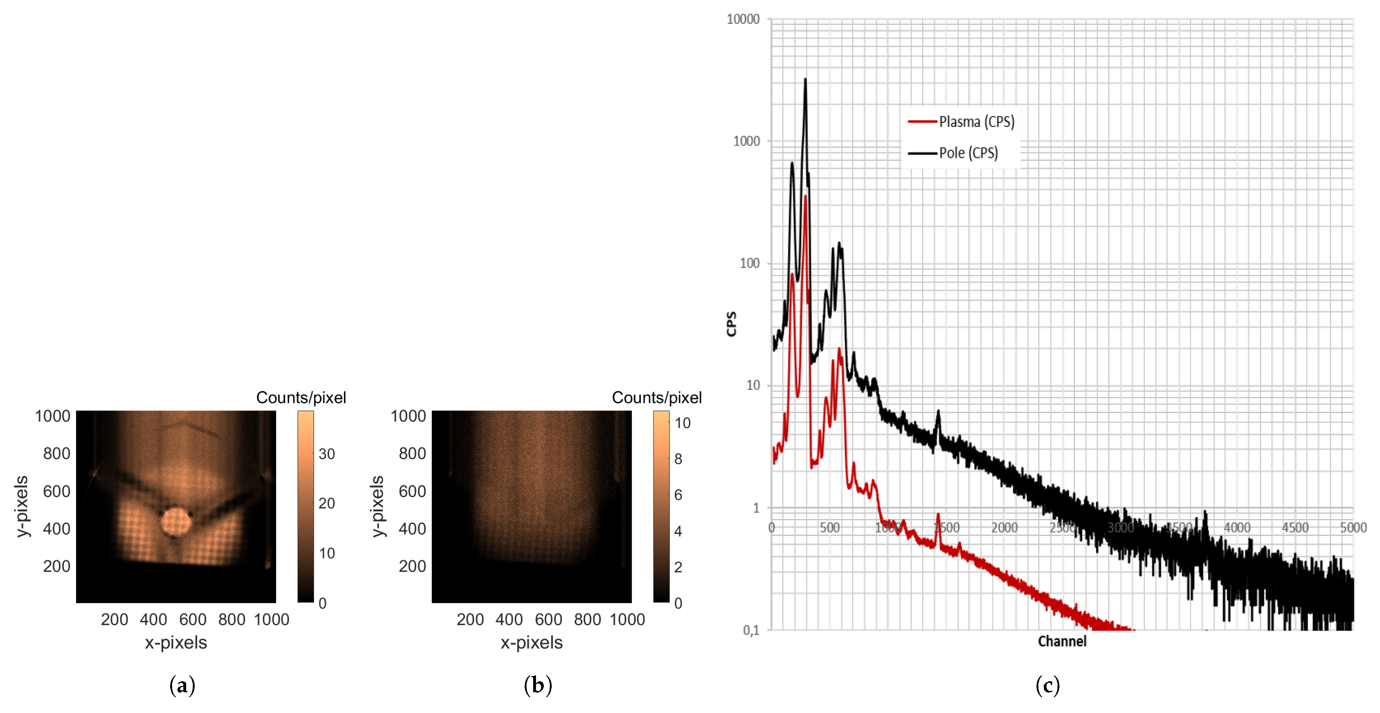
2. The Experimental Setup

The measurements were carried out with a room-temperature, second-generation ECR ion source installed in the ECR Laboratory of ATOMKI (Debrecen), based on a B m i n i m u m magnetic field configuration—characterized by the superposition of an axial magnetic field (from axial coils) and a radial magnetic field (from hexapole coils)—using a basic operation pumping frequency of 13.9 GHz at a power of 200 W. The axial magnetic field in the plasma chamber was 1.26 T (injection side entering point), 0.39 T (in the center, B m i n i m u m ) and 0.92 T (extraction side exiting point), whilst the radial magnetic field produced by a permanent magnet closed cylindrical hexapole and measured at the plasma chamber wall (R = 29 mm) was 1.1 T. The length of the plasma chamber was 210 mm, and the internal diameter was 58 mm. The ion source was optimized for middle-charged argon ion production, while the gas pressure measured at the injection box of the ion source was 2 × 10 6 m b a r .
The diagnostic setup used to perform high-resolution X-ray imaging is shown in Figure 1a. The CCD X-ray camera (model Andor, iKon-M SO series) was made of 1024 × 1024 pixels, with an optimal quantum efficiency in the range 0.5–20 keV. It was coupled to a Pb pin-hole (thickness 2 mm, diameter Φ = 400 μ m) placed along the axis, facing the chamber from the injection flange. A titanium window with a thickness of 9.5 μ m was used to screen the CCD from the visible and UV light coming out from the plasma.
In order to work with the ECR-plasma heated at a high power, the overall pin-hole system was redesigned, including a multi-disk lead collimator for the extra shielding of scattered radiation. The multi-disk collimator consists of two lead disks with the same thickness (1 mm) and different diameters Φ (2 mm, 1 mm). The lead pin-hole was placed between the two lead disks, which were located at distances of l 1 = 40 mm from the pin-hole at the CCD side and l 2 = 6 mm far from the pin-hole at the plasma side. The optical magnification M was optimized to be M = 0.244 (distance p i n h o l e C C D = 232 mm, distance p i n h o l e p l a s m a c e n t r e = 952 mm). Other details about the setup are described in [28].
In this system, the pin-hole camera was operated up to 200 W of total incident power in the plasma—namely, one order of magnitude higher than previous measurements (where the pumping power was limited to 30 W [17,18]). In this way, both stable and turbulent plasma regimes (typically triggered above certain power thresholds [29,30]) were investigated [31], as well as new plasma heating methods [32,33,34].
To allow for SPhC-based, quantitative, space-resolved spectral analysis, the ATOMKI plasma chamber walls were covered by thin layers of materials with different X-ray fluorescence energies, whilst the plasma was made by Ar, with a fluorescence emission at around 2.96 keV. In this way, even in energy-integrated images, the X-rays coming from the plasma are clearly visible, while the materials of the extraction (titanium) and injection (aluminum) endplate and of the lateral walls (tantalum) provide bright regions of X-ray emission due to bremsstrahlung and X-ray fluorescence.
The sketch of the ATOMKI plasma chamber is illustrated in Figure 1a (on the right). This figure reports the shape of the plasma core, the so-called “plasmoid”, which is typically contained within the iso-magnetic surface fixed by the ECR condition ω R F = q B / m , where ω R F is the RF pumping frequency, B is the magnetic field and q and m are the electron charge and mass, respectively. From this high-density core, fluxes of deconfined electrons and ions escape, according to the so-called “loss cones”. The field lines lying inside the loss cones are represented in white and yellow. Small bullets of different colors represent the lost electrons moving towards the lateral chamber walls (red dots) or towards the endplate (yellow dots).
The perspective front-view of the plasma chamber (i.e., the same view as the pin-hole camera setup) is sketched in Figure 1c. The Al mesh (with a wire diameter of 400 μ m) that was placed on the injection endplate to keep the microwave resonator-like properties of the plasma chamber is clearly visible, allowing for direct inspection of the chamber interior, guaranteeing more than 60 % of optical X-ray transmission.

3. X-ray Spectrally-Resolved Imaging Algorithm

Each photon impinging in the CCD camera releases its energy in the silicon, generating a characteristic number of photo electrons, proportional to its own energy. The Analogue Digital Unit (ADU), corresponding to the information read by the CCD in each pixel, is, therefore, proportional to the product of the incident photons by their energies. We adopted two operative modes to acquire the images: the Spectrally Integrated mode and the SPhC mode.
Images obtained with long t e x p (tens of sec) are called Spectrally Integrated images: in this case, no energy discrimination is possible (but they are useful anyway, since the ADUs are related to the energy content of the plasma). These acquisitions are relatively fast and it is possible to monitor “on line” changes in the plasma structures or plasma losses on the chamber walls. A typical example of a Spectrally Integrated image is shown in Figure 1b. This image was collected with an exposure time of 50 s, at 1 MHz of readout rate using the full-frame (1024 × 1024 pixels) acquisition mode. Regions of Interest (ROIs) in the images were individuated according to the expected structure of the ECR plasma in B m i n i m u m magnetic field traps, as sketched in Figure 1a. Figure 1b shows several bright regions due to plasma and plasma chamber wall emissions. The aforementioned ROIs, in light of the detailed description of the Figure 1a, are reported here, including:
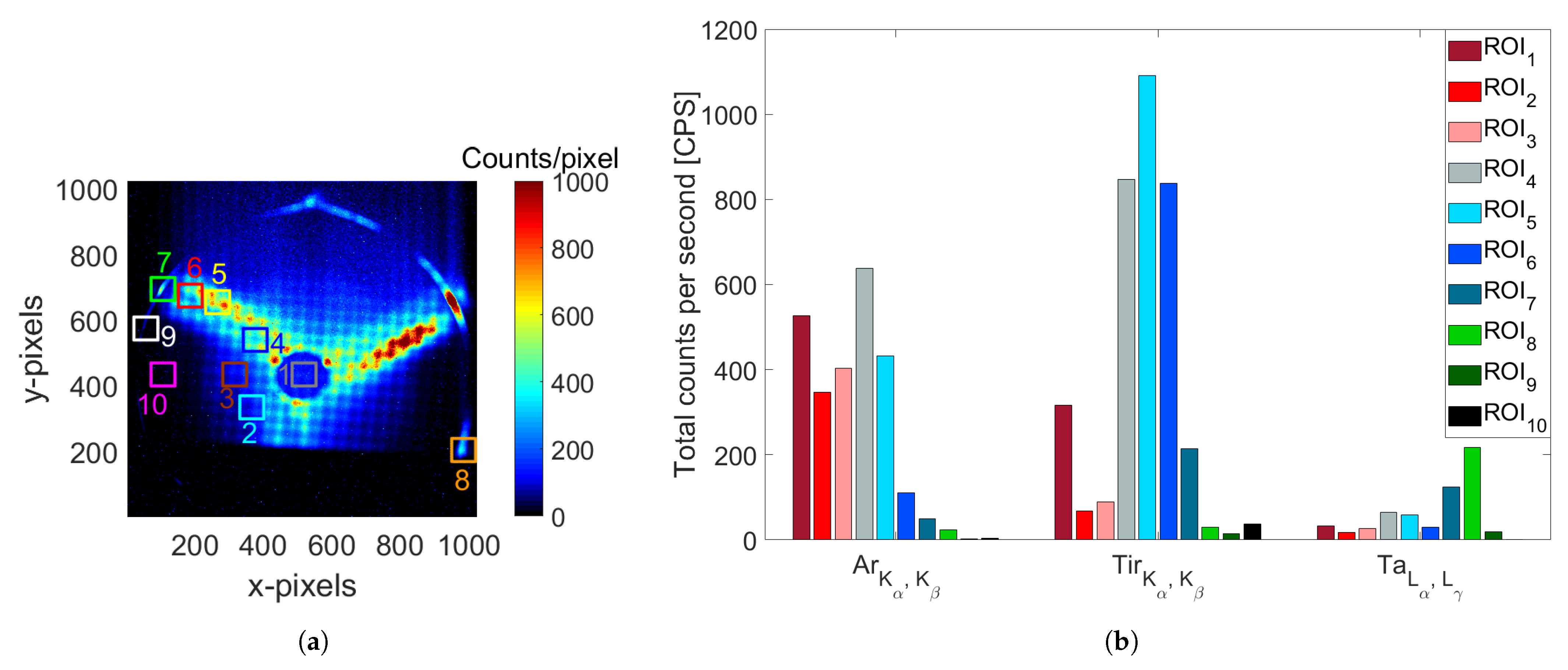
  • White rectangles, enclosing the regions where the X-rays come from the plasma region (i.e., there are no perspective interceptions with the chamber endplates beyond them);
  • Black squares, highlighting the so-called “magnetic branches”, i.e., the bremsstrahlung-produced X-rays and X-ray fluorescence coming from extraction endplate, due to electrons escaping axially (shown in yellow in the pictorial view of Figure 1a);
  • Bright green squares, indicating the regions where the magnetic field lines intercept the lateral walls of the plasma chamber (the ones depicted in red in Figure 1a).
This plasma image demonstrates this method’s ability to qualitatively separate the X-ray radiation coming from the plasma from that coming from the plasma chamber walls, but the more powerful investigations, which are able to perform local energy determination, are provided by the SPhC mode.
To operate in SPhC mode, the development of proper acquisition and post-processing procedures was required.
The SPhC mode is obtained by fixing a very short t e x p for each of the acquired image frames (several tens of milliseconds), minimizing the probability that two (or more) photons hit the same pixel or its nearest neighbors.
SPhC t e x p was empirically set-up in such a way that only a few pixels were illuminated on the full CCD matrix during a single-frame acquisition; a sequential acquisition of thousands of SPhC frames then allows us to obtain the statistics necessary for obtaining high quality X-ray fluorescence spectra and images.
The developed analytical post-processing method was developed in MatLab, and consists of five different steps:
(I)
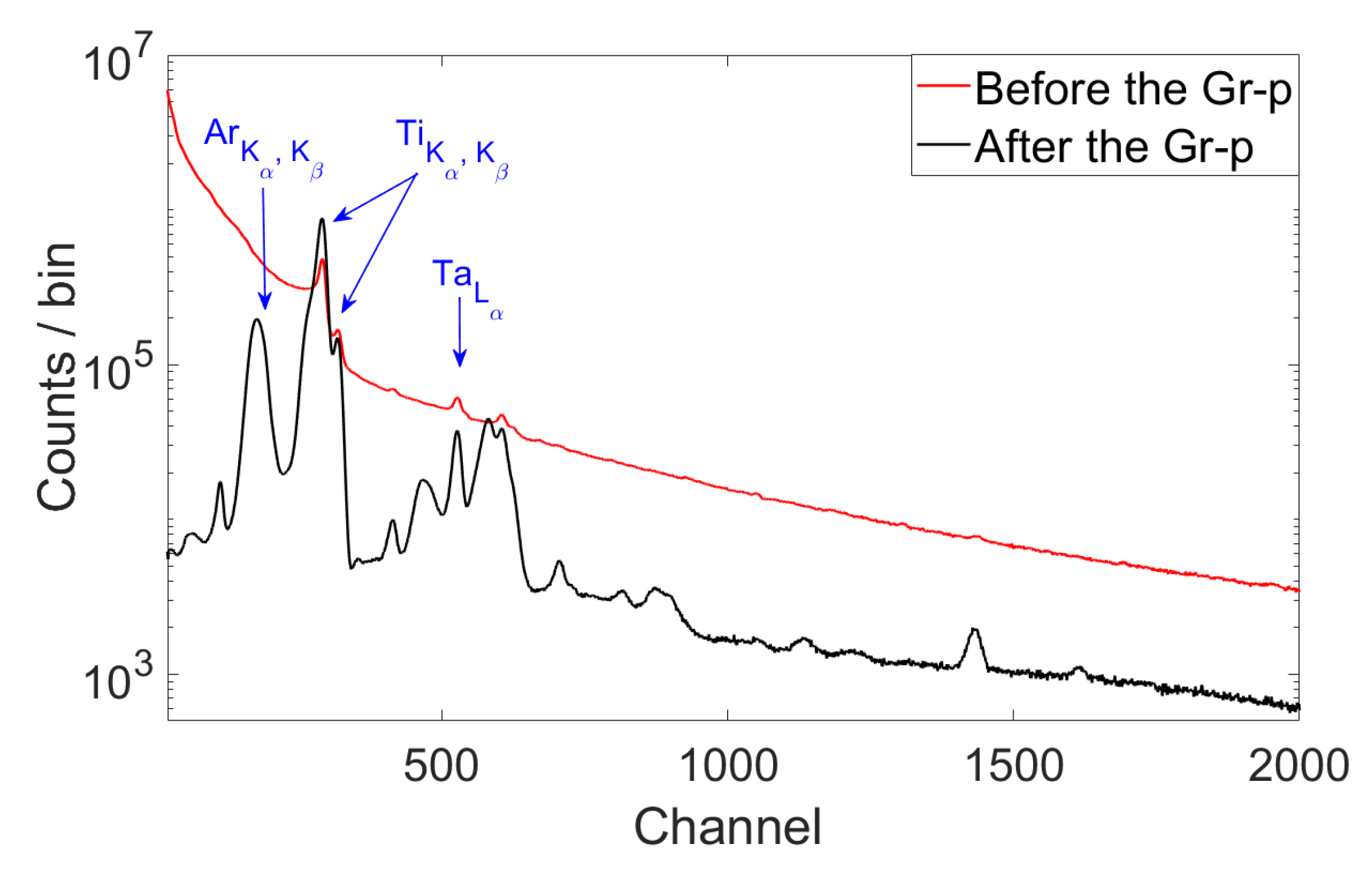
Grouping process (Gr-p);
(II)
Energy calibration and event counting normalization;
(III)
Energy filtering process;
(IV)
High Dynamical Range (HDR) imaging and spectroscopy;
(V)
Readout Noise (RON) removal (RON-r).
The details of each step are described, respectively, in the following five subsections.

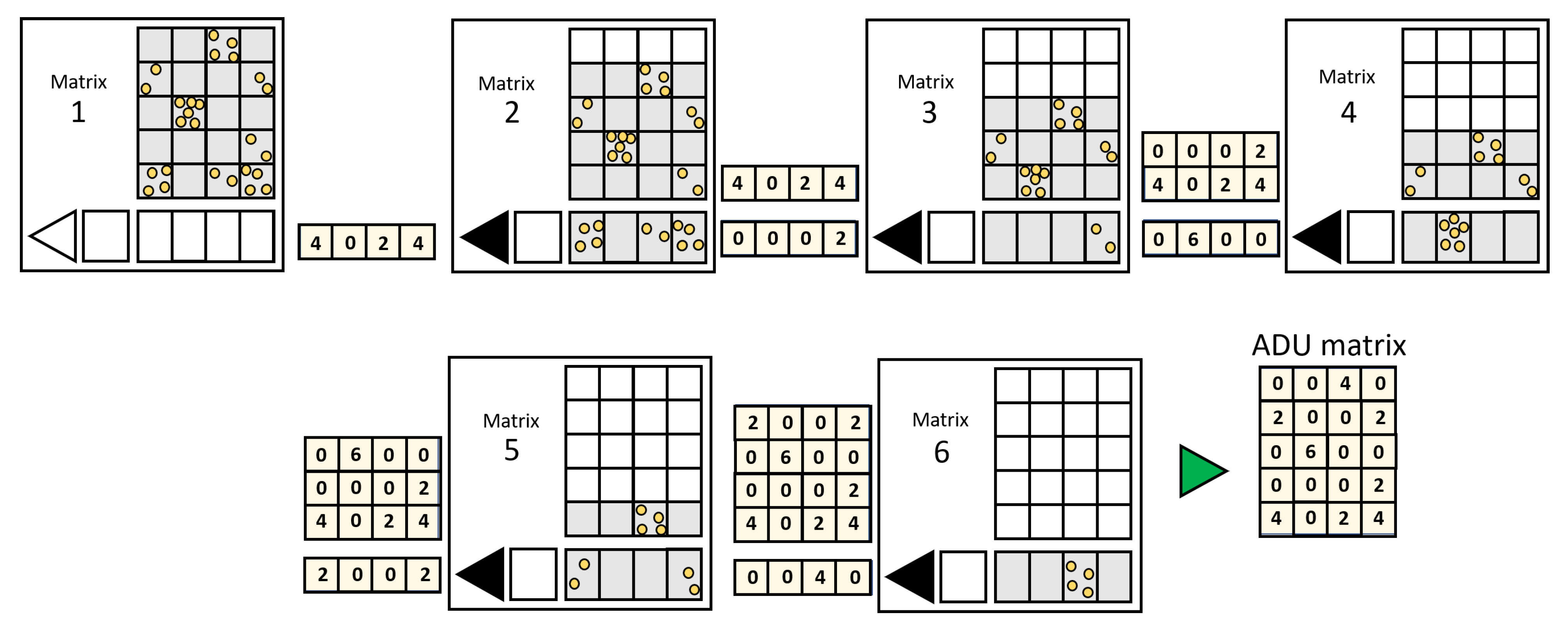
3.1. The Grouping Process

Even working in SPhC mode, some pixel-clusters are often in each of the acquired image frames: they could be associated with a single photon that interacts with more than one pixel or with two (or more) photons hitting neighboring pixels. The grouping process (Gr-p) aims at finding real SPhC clusters, discarding spurious events.
For this purpose, we introduced the S parameter representing the maximum cluster size (defined as the number of neighboring pixels in a cluster) that can be considered to be due to a single-photon event. Clusters larger than S are filtered out. The noise contribution is removed by setting a threshold L.
In more detail, the algorithm works in the following way:
STEP-1: 
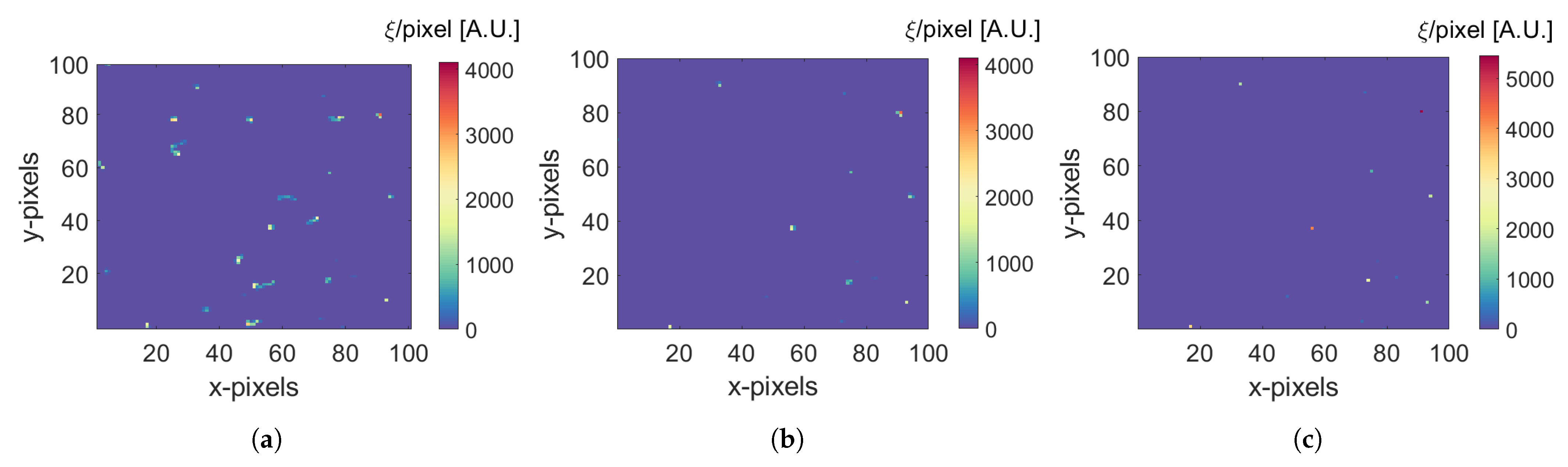
Considering a given image-frame J, all pixels with an ADU < L are “turned off”; then, for a given J frame, neighboring pixels of an illuminated pixel at coordinates ( X , Y ) J are checked. In case there are no charges in the surrounding pixels, the event is considered to be purely a single photon and is associated with three coordinates ( X , Y , E ) J , with E being the energy associated with the photon (determined as in Section 3.2). This is shown in Figure 2a;
STEP-2: 
When a group of active neighboring pixels (a cluster) is identified, the algorithm tries to distinguish single from multiple-events:
(a)
Single photon-event clusters are typically characterized by a single, clear maximum: for these, in STEP-3, described below, we see that the code associates the integrated total charge to a single photon energy, whose ( X , Y ) J coordinate corresponds to the maximum;
(b)
Clusters associated with multiple-hit events (showing different relative maxima in a big-size cluster) are filtered out from SPhC images. However, the algorithm stores the information anyway, labelling them spurious events (in SPhC images, their value is set at zero);
STEP-3: 
Charges of all those pixels belonging to non-spurious clusters (see Figure 2b) are integrated to provide energy-position information of single-photon events (reported in Figure 2c).
In Figure 2, a ROI of 20 × 30 pixels has been processed by Gr-p with S = 5 and L = 10 as input parameters.
Figure 3 reports the corresponding images (here, obtained considering a larger ROI of 100 × 100 pixels) after the application of the grouping algorithm.
After the application of the Gr-p process to the whole dataset, N becomes the number of photons with energy E in the position (X, Y). Therefore, the four-dimensional array ( X , Y , E , N ) is obtained. Integrating over the spatial coordinates (X, Y), we obtain the N t o t versus the energy E plot; i.e., the full X-ray spectrum. This latter is reported in Figure 4. The figure shows the full-field X-ray spectrum collected from a plasma obtained at 200 W of RF power and 13.90 GHz of RF frequency.
In this figure, the raw spectrum (red line) is compared with the Gr-p post-processed one (in black). Fluorescence lines of Ar, Ti and Ta (coming from plasma and plasma chamber walls) are visible only in the post-processed plot.

3.2. Energy Calibration and Counting Normalization

To perform the energy calibration, four characteristic peaks corresponding to the T i K α , T i K β , T a L α and T a L γ fluorescence peaks, were considered. The energy and channel values of each peak are summarized in Table 1 and the linear correlation coefficient of the linear fit results R = 1.
The calibrated spectrum, expressed in a logarithmic scale, is shown in Figure 5a, whilst an enlargement of the energy range 1–15 keV, where all characteristic peaks are highlighted by labels, is shown in Figure 5b. Fluorescence peaks (the K α and K β of titanium, the L α , L β , L γ and M α of tantalum) and of the plasma ( K α and K β of argon) are highlighted by appropriate labels.
The estimated energy resolution is 0.326 keV at 8.1 keV (corresponding to the T a L α line).
Dimer and escape peaks of the silicon-made CCD are also visible. This latter peak is an artifact, due to the probable S i K α X-ray photon generation inside the detector: these photons can escape from the detector volume, thus reducing the effective detected energy of some incident rays by ∼1.74 keV ( S i K α X-ray energy). The escape peak coming from Ti fluorescence overlaps with the A r K α fluorescence. Consequently, methods to minimize these contributes have been also implemented. Several papers [35,36,37] have demonstrated that the escape peak generation efficiency is typically of the order of 3 % of the main K α peak. Thus, the algorithm considers an escape peak efficiency Z of the 3 % of the main T i K α peak and removes this contribution pixel-by-pixel, in both the whole matrix and the spectrum.
Moreover, in order to remove the bremsstrahlung continuum radiation generated by the deceleration of the energetic electrons colliding with heavy ions in the plasma and with the atoms of the plasma chamber walls, an exponential fit was performed in the range of 30–100 keV (which corresponds to the red line in Figure 5a).
Finally, spectra need to be renormalized, including both the quantum efficiency (Q.E.) of the CCD camera (absorption efficiency in 15 μ m of Si) and the transmission efficiency through the titanium windows (9.5 μ m of Ti thickness): this was done by means of the NIST database [38]. The total detection efficiency, called F(E), was obtained by multiplying the quantum and the transmission efficiencies. The three curves are shown in Figure 6a. All event counts are normalized, dividing them for F(E). One example of the event-count-normalized spectrum is shown in Figure 6b.

Optimization of the Algorithm

The spectrum shape and intensity changes as a function of L and S values were optimized in an attempt to reach a trade-off between spectral resolution and sufficiently high statistics. In Figure 7a, five different spectra evaluated by setting different S values (from 1 up to 5), fixing L = 10, are shown (in the energy range 1–15 keV). The spectra in the whole energy range are instead shown in Figure 7b.
We find that at the lowest S, the spectrum shows higher resolutions but also the lowest intensities. In addition, since at the lowest S, we have an overfiltering of larger clusters, the maximum energy (consequently, the electron temperature that is inversely proportional to the spectrum slope [13]) decreases as a function of S, as shown in the Figure 7b.
To account for these effects, and to reduce the impact of dimer and escape peaks, the implemented algorithm optimizes the input S and L parameters (we set three L = 5, 10, 15 values: for L = 5 and L = 15 the code run for five values of S = 1–5, for the case L = 10 we have S from 1 to 10) to improve the I M P I E P and I M P I D P ratios as much as possible (where I M P , I E P and I D P are, respectively, the main peak intensity, the escape peak intensity and the dimer peak intensity).
Optimization was searched by a trade-off between overall statistics and the minimization of spurious peaks (escape, dimer, triplet, etc.).
For each configuration, the following three values were estimated:
(a)
The I M P I E P ratio for T a L α ;
(b)
The I M P I D P ratio for T i K α ;
(c)
The total I M P for T i K α ;
From the analysis, we find the following:
(a)
The escape peak intensity vs. the main peak intensity is almost independent of L and S;
(b)
The dimer peak intensity dramatically increases with respect to the main peak when increasing the cluster size;
(c)
The intensity of the spectral components (e.g., I T i K α ) increases with S.
By adding the same relative weight of the three optimization procedures (low escape, low dimer, high intensity), the optimal values were L = 10 and S = 2. In case of low statistics, L = 10 and S = 5 were found to be the best compromise.
In summary, the whole process described in the previous sections (i.e., from raw data to calibrated and optimized spectra) is summarized in the sketch shown in Figure 8.

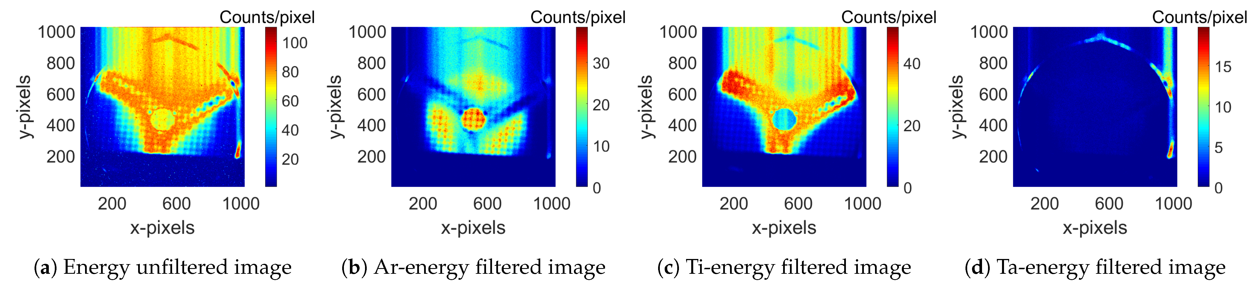
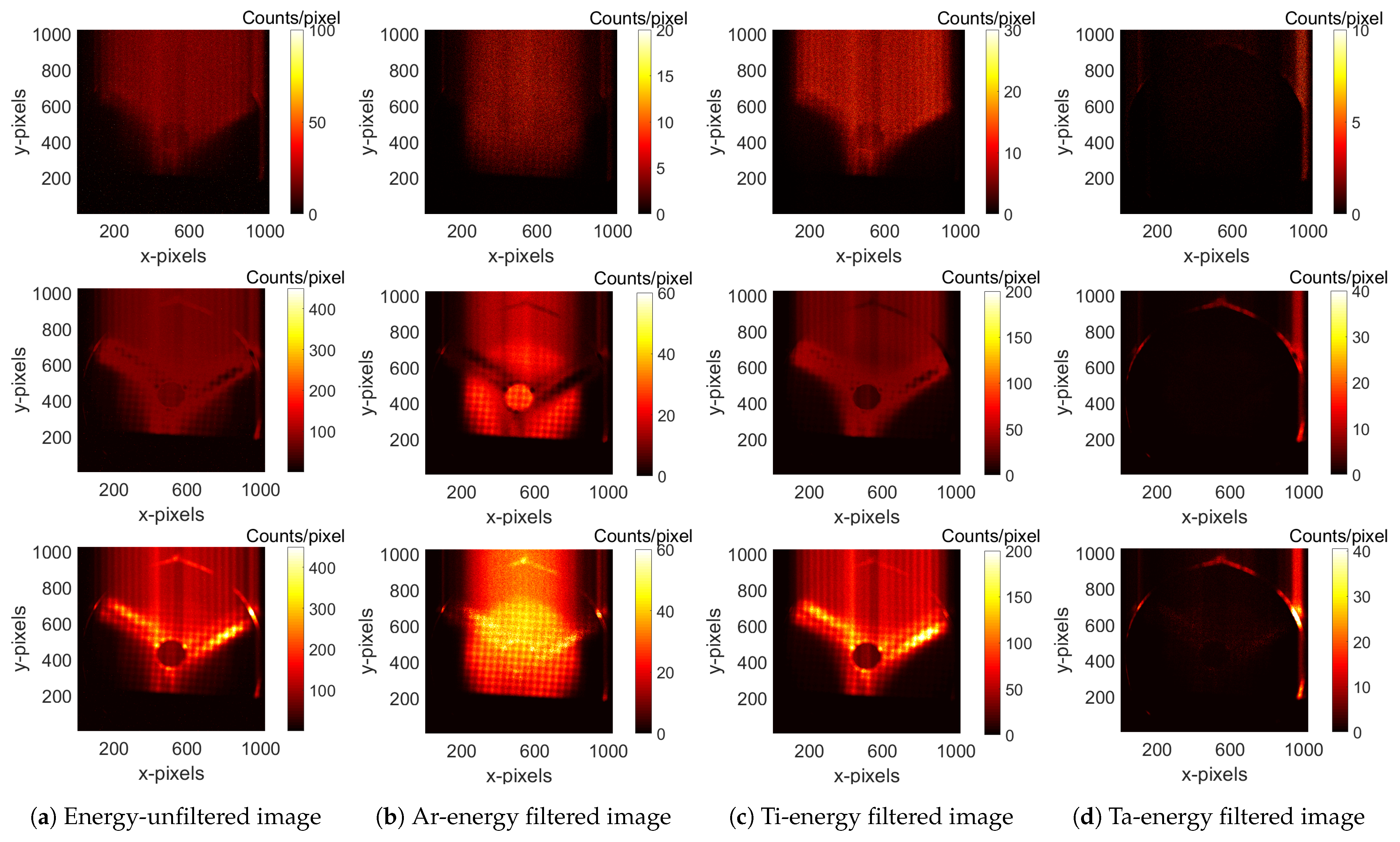
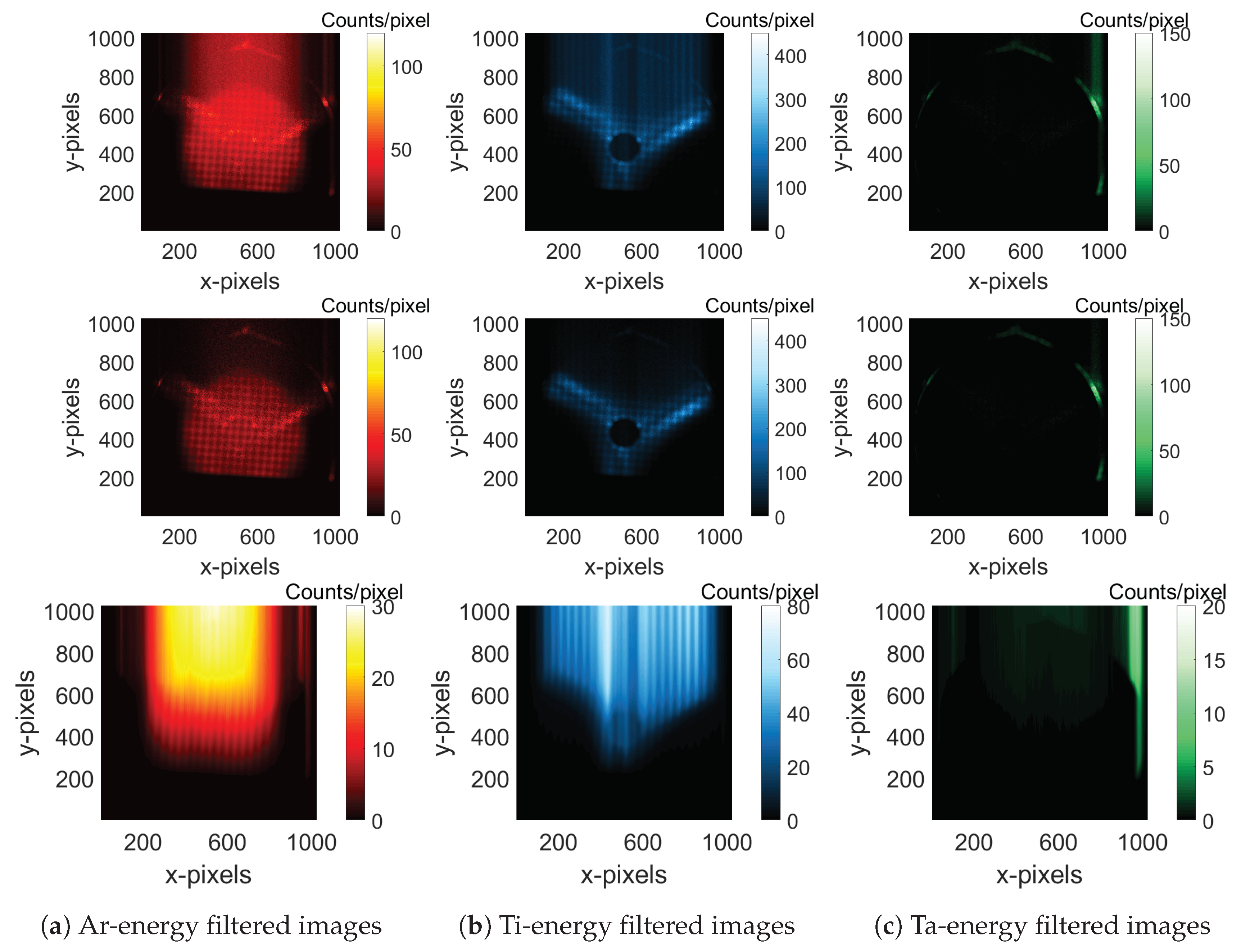
3.3. Energy Filtered Images

Let us now consider, as an example, the image shown in Figure 9a. The image is the result of the analysis of a number of image-frames N f r = 4200 acquired with t e x p = 500 ms, at a 1 MHz readout rate and full-frame ( 1024 × 1024 pixels) acquisition mode. The spectrum of the full-size image is the one shown in Figure 7a (for S = 5 and L = 10). The energy-filtered imaging consists of selecting only those pixels that were loaded by only those photons with energy in a given energy interval Δ E .
We plotted images using Δ E corresponding to the fluorescence peaks of Ar, Ti and Ta, respectively, in Figure 9b–d.
In other words, looking at the structure of the plasma and chamber depicted in Figure 1a, the images in Figure 9 only display the emission coming from Ar plasma; the effect of electrons lost by the magnetic confinement on the radial walls is visible through the Ta fluorescence, while the axial losses are visible through the Ti fluorescence.
In Table 2, the selected investigated energy intervals are summarized.

3.4. High Dynamical Range (HDR) Imaging and Spectroscopy

When local emissivities of an image vary, even on orders of magnitude, it is very challenging to determine the correct t e x p to avoid extra or under-exposure. The solution comes from the HDR analysis—commonly used in visible light imaging—which consists of acquiring the same image, setting two or more different t e x p , and then producing a weighted, convoluted image.
In our case, Spectrally Integrated images at t e x p = 50 s (see Figure 1b) display Ar intensities of lower orders of magnitude than magnetic branches or poles. The same happens in SPhC mode.
In this latter case, we optimized t e x p and N f r acquiring different datasets, considering the hugely different local emissivities. In particular (see Table 3), we used t e x p = 0.5 s, which was able to obtain good photon counting changes in the low-intensity ROIs, acquiring a total of 4200 frames. These images were called I P l a s m a .
t e x p = 0.05 s and 1000 frames were instead set to have an optimal SPhC in ROIs showing higher emissitivities: these were called I P o l e .
As an example, two event-counted single full-frames (before applying the Gr-p) are shown in Figure 10a,d for I P l a s m a and I P o l e , respectively.
It is possible to notice the difference from I P l a s m a and I P o l e considering two ROIs:
  • The plasma ROI: Red square in Figure 10a,d, where the enlargement is shown in the images in Figure 10b,e for I P l a s m a and I P o l e , respectively. In this ROI, both the I P l a s m a and the I P o l e frame are photo-counted, but only the I P l a s m a frame shows a high enough statistic, whilst in the I P o l e frame, it is too low.
  • The magnetic pole ROI: Cyan square in Figure 10a,d, where the enlargement is shown in the images Figure 10c,f for I P l a s m a and I P o l e , respectively. In this ROI, the I P l a s m a frame is not photon-counted, whilst the I P o l e frame is photon-counted and the loaded clusters are isolated.
After applying the Gr-p and summing over all event-counted frames, the images shown in Figure 11a,b, for I P l a s m a and I P o l e acquisition mode, respectively, were obtained (the frames were also Ar-fluorescence energy-filtered). As expected, the I P l a s m a image shows a lack of information in the magnetic branches and poles’ ROIs.
The correspondent spectra (called basic spectra) normalized by t e x p and N f r are shown in Figure 11c. The I P l a s m a spectrum shows some missing (and under-represented) information as well. Here, the total rate (CPS, counts per second) is about one order of magnitude lower than the total rate (CPS) of I P o l e . In this condition, it is necessary to combine two images and spectra into a single image and spectrum, respectively, by means of the High Dynamical Range procedure.
Since the degree of the missing information is spatially dependent, the implemented algorithm operates by exploring any pixel in each image-frame, as was performed for the Gr-p, but, in this case, the goal is to define two “masks” that are necessary to obtain the HDR image:
  • HDR Mask: This mask shows those pixels which were not photon-counted on I P l a s m a images. It consists of a digital (0–1) array, where a position evaluated as 1 corresponds to those pixels that are part of a cluster larger than the S parameter, for each image frame. The sum of those images, divided by N f r , gives the desired HDR Mask, where each number corresponds to the probability ρ p l n p h c normalized to 1 of a given pixel to be not photon-counted, as shown in Figure 12a.
  • Pole normalization Mask generation from I P o l e frames: Even the I P o l e frames are not always photon-counted; therefore, the counts are under-represented and the missing information is spatially dependent. Using the not-photon-counted matrix (NPhC) obtained from the I P o l e images ( ρ p o l n p h c ), a normalization matrix was obtained (shown in the Figure 12b): Normalization matrix = 1/(1 − NPhC/1000).
  • HDR image = I P l a s m a + I P o l e × HDR mask × Pole normalization mask. Of course, I P o l e was normalized for t e x p and N f r . The HDR image is shown in the Figure 13.
Observing the Figure 13, it is clear that the HDR image—compared to I P l a s m a and I P o l e —contains all the information, with a good statistic in the plasma, magnetic branches and poles ROIs. Pixels clusters that in I P l a s m a were filtered out by the Gr-p were replaced by those taken from the I P o l e , once weighted by the HDR and pole normalization masks. Of course, the same analysis can also be performed in the energy-unfiltered image and in the other energy-filtered images (for titanium and tantalum), as shown in Figure 14.
Finally, a similar HDR procedure was applied to the basic spectra as well.

3.5. The Readout Noise (RON) Removal Algorithm

During the readout time t R O of the CCD camera, the accumulated charges are transferred through the CCD rows from the top to the bottom, where the reading buffer is placed. During this transition, the CCD is still active, and is therefore sensitive to the impinging photons. This implies that, during the readout, some photons are still detected, but in the “wrong place”, this effect causes the vertical “strips” visible in the images, as is possible to observe in Figure 14. If the t R O t e x p , the readout noise (RON) is comparable to the real signal. Thus, its contribution has to be managed, i.e., removed or—if possible—recovered, since the acquisition even during the readout process is genuine, despite being mismatched in position. A proper algorithm to handle this effect was written and applied.
In Figure 15, the ADU matrix loaded by the CCD in the case that the RON was neglected is shown. However, considering the RON contributions, the ADU matrix drastically changes, as is possible to see in the Figure 16. In the case shown in Figure 16, an impacting RON flux equal to half of the initial flux during the readout time of one row ( t R O r ) has been considered. This fraction (0.5, in this example) is called β .
In more detail, in Figure 16, matrix 1 shows the initial photons flux (yellow dots) impacting in the CCD. During the first row readout time, an additional contribution, due to the RON flux, impacts in the CCD (red dots in the matrix 2), and it is half of the initial photon number since we considered β = 0.5 . In matrix 3, another RON contribution (blue dots) impacts during the second row readout time. The same happens in matrix 4 (green dots), and so on. Hence, the final ADU matrix (real case) dramatically differs from that where the readout noise was neglected (ideal case).
The developed algorithm, once given the amount of time needed for information transfer between the rows and the standard acquisition time of the CCD, starts by identifying the amount of photons collected in the “wrong” position, considering the spatial distribution of the photons collected in the exposure time (step-1); once identified as wrongly collected photons, the algorithm reallocates them in the correct positions (step-2).

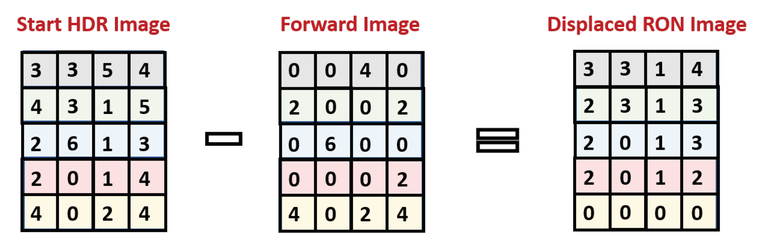
3.5.1. Step-1: The Forward Method

The first step of the algorithm (called the Forward Method) consists of filtering out all the charges due to RON photons, which are pixel-position-dependent. The algorithm works, as shown in the example in Figure 17.
Considering the Start HDR Image, only the first row (yellow backgrounded) is unaffected by the RON, since it is read instantaneously. The second row (red back-grounded) contains both the charge due to the impact of photons and the additional RON due to the impact of photons during its t R O , proportional to the flux that can be estimated by the previous rows (only the first one, in this case). The third row (blue backgrounded) contains the charges due to the impact of photons plus two additional RON contributions, proportional to the fluxes read in the previous two rows, and so on. The algorithm, starting from the Start HDR image, subtracts the RON contribution step-by-step in each row that was loaded during the t R O .
Starting from the Start HDR Image (the first image), 1023 images were analyzed step-by-step: the Kth image (with K = 2 → 1024) corresponds to the ( K 1 ) th image, in which all rows j (with j K ) we resubtracted by a contribution that was proportional (of a factor β ) to the loaded charge in the ( K 1 ) th row of the I m a g e K 1 . In the final post-processed image, called Forward Image, all RON contributions were filtered out. The Forward Image is characterized by the same ADUs of the image that was obtained by neglecting the RON contribution (Figure 15), demonstrating the effectiveness of the described procedure.
Moreover, considering the difference between the Start HDR Image and the Forward Image, it is possible to obtain the so-called “Displaced RON Image” consisting of all RON photons that were collected during the RO time and placed in incorrect positions (see Figure 18).
These RON photons on the one hand represent a spurious contribution because they are placed in the incorrect pixel position; on the other hand, they are “good” events because they are true photons coming from the plasma setup that impact the CCD. It was possible to relocate them in the correct pixel position, increasing the statistics.
In the previous example, a β parameter of 0.5 was considered, but the real experimental β parameter (which depends on the t R O ) was estimated. The measurements were performed, setting a readout frequency of 1 MHz ( 10 6 pixels/sec); therefore, the readout time of a single pixel t R O p is 10 6 s, and, subsequently, the readout time of one row R O t r was found to be 1024 × 10 6 = 0.0010124 s. Therefore, the β parameter is
β = t R O p t e x p
where β represents, in other words, the fraction of flux impacting a single row during its own t R O . For I P l a s m a , where t e x p = 0.5 s, β I P l a s m a = 0.002 ; whilst for I P o l e , where t e x p = 0.05 s, β I P o l e = 0.02 . The measured Start HDR, Forward and Displaced RON images are shown in Figure 19a–c for Ar, Ti and Ta energy-filtering, respectively.

3.5.2. II Step: The Backward Method

The genuine events shown in the Displaced RON Images (Figure 19, bottom row) must be “relocated” in the correct position by means of the second step.
Thus, a new matrix, called the Weight Matrix (WM)—obtained by multiplying the Forward Image by β —was defined. A sub-matrix W i was associated to each ith row, normalized and expressed as a percentage (with nonzero elements only in rows j i ). The elements of the W i matrices give the pixel-position-dependent weight w k , j of the RON that comes from each pixel during the readout time.
The second step of the algorithm consists of redistributing the charge loaded in each pixel ( i , j ) of the Displaced RON Image, in all the pixels ( k , j ), with k = ( i + 1 ) → 1024, of a new matrix called R O N i by means of the weights w k , j . The W i and R O N i are shown in Figure 20, for i = 1 t o 4.
The sum of all the R O N i matrices gives the so called “Placed Readout-Noise Image”, shown in Figure 21, which corresponds to the Displaced RON Image where all charges are redistributed in the correct pixel-position. It is possible, in fact, to verify that the total charge is the same: the total ADU is 31 both in Placed RON Image and in Displaced RON Image (see also Table 4 to compare the ADU values of the experimental acquired images).
Even if the Forward Matrix can be used to calculate the Weight Matrix, as shown in the previous example, it is possible to demonstrate that there is an improvement when replacing it with the one obtained by applying a pixel-position-dependent threshold in the Forward Matrix. The reason for this is that there is also a background (BGN) contribution during RO acquisition.
In this context, a pixel-position-dependent threshold was defined and applied in the Forward Matrix:
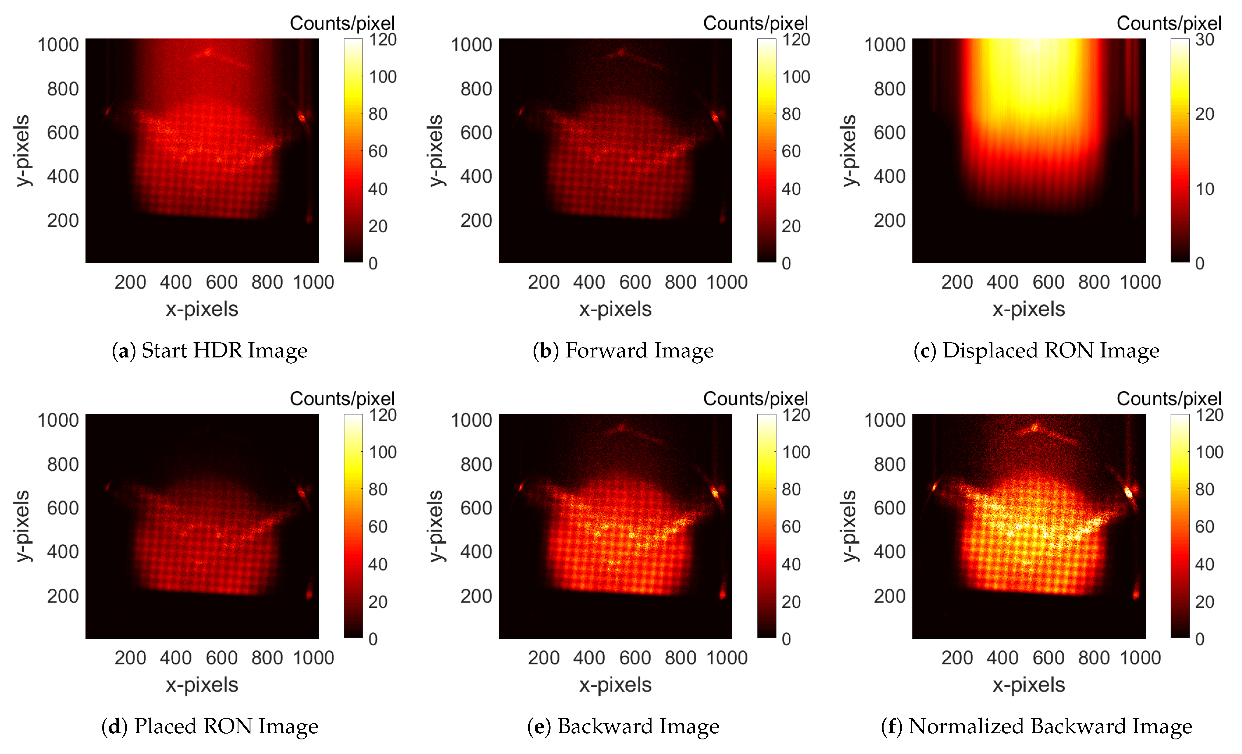
  • First, 200 image frames acquired setting the lowest t e x p possible in the driver ( t e x p = 20 μ s) were used to estimate the BGN threshold. The sum of the 200 event-counted frames is shown in Figure 22a, which was normalized for the frames number, and the σ level, pixel-by-pixel, was considered the BGN threshold (Figure 22b).
  • The Start HDR, Forward and Displaced RON images are shown in Figure 23a–c, respectively.
  • Setting the BGN threshold in the Forward Image, the Weight Image was obtained and used to estimate the Placed RON Image (Figure 23d). It contains the same RON charge as was collected in the Displaced RON image, but placed in the correct positions.
  • The sum of the Forward Image and of the Placed RON Image gives the so-called “Backward Image”, shown in Figure 23e, which contains the whole charges (collected during the measurement time + RON time) in the correct pixel-positions.
  • For the data collected during the RO, the effective t e x p is pixel-position-dependent; therefore, the Backward Image was also properly time-normalized. The final post-processed image is called the “Normalized Backward Image” and is shown in Figure 23f.
The images shown in Figure 23 are argon energy filtered.
It is worth highlightig that the post-processed image quality dramatically improves compared to the original quality. The proper handling of RON after the elaboration of the “Normalized Backward Image” is evident, and the spatial resolution increases.
In Table 4, it is possible to observe that the total counts of the Start HDR Image (a) are the same as those of the Backward Image (e): the only difference is that all the RON photons were relocated in the correct positions. The same observation can be made for the Displaced RON Image (c) and the Placed RON Image (d). The sum of the total counts of the Forward Image (b) and the Displaced RON Image (c) is equal to that in the Start HDR Image (a). The slight difference between the counts of the Weighing Image (i) and the Forward Image (b) is due to the events filtering after the elimination of the BGN.
We calculated the total counts in a R O I S I G N A L that was almost completely unaffected by the readout noise (i.e., the signal in R O I 2 ) and the total counts in a R O I R O N in a region outside the plasma chamber dominated only by readout noise (i.e., positioned at the top-center of the image). The signal-to-noise ratio was calculated in four different images corresponding to those obtained after applying the four different RON-r methods. The comparison is reported in Figure 24, highlighting the comparatively huge improvement (a factor of 30, compared to the original image) obtained after the implementation of the entire sequence of algorithms.
The corresponding Ti and Ta energy-filtered images are shown in the Figure 25 and Figure 26, respectively.
Finally, in Figure 27, the comparison between the I P l a s m a images, the HDR post-processed images with RON and the Readout Noise Removed post-processed images is shown (note that the full scale is different in the I P l a s m a images compared to the others). Event counted energy unfiltered images (Figure 27a), Ar energy-filtered images (Figure 27b), Ti energy-filtered images (Figure 27c) and Ta energy-filtered images (Figure 27d) are shown.
It is possible to observe the improvement in the final post-processed images, where the “strips” due to RON have completely disappeared. First, plasma properties investigations, performed by applying the whole set of algorithms described above, are reported in [39].
The error analysis of the number of counts in each pixel of the single-photon counted-image was estimated by the square-root of counts. The Figure 28 illustrates, for each pixel, the relative error σ r e l of the counts for the event-counted, Ar-filtered image (Figure 28a) and for the event-counted, Ti-filtered image (Figure 28b). The relative errors are < 10 ÷ 15 % in the plasmoid and lower than < 4 ÷ 8 % in the magnetic branches regions. In the magnetic poles, the relative errors are around 10 % . These are the typical uncertainties of the number of counts in each pixel, which affect the performed measurements. These numbers correspond to single pixels. Due to the high resolution, we can easily (without a remarkable loss in spatial resolution) increase the statistics, and consequently decrease the uncertainty, by summing up a group pixels corresponding to a given ROI.

4. Plasma Analysis: A Short Overview

After post-processing the X-ray images by means of the advanced algorithm, two important complementary analyses of the SPhC images can simultaneously be performed: (a) HDR energy-filtered imaging and (b) HDR space-filtered spectroscopy.
By means of the HDR energy-filtered imaging, it is possible to obtain the imaging of the elemental distribution, distinguishing the emission and the corresponding image coming from each material. Pixels highlighting photons due to fluorescence peaks are shown in the last columns of Figure 27b–d, respectively, for the Ar, Ti and Ta-energy-filtered images. In this way, it is possible to study the plasma structure and morphology changes and to investigate the plasma confinement and losses dynamics in detail.
A complementary analysis consists of the selection of a ROI in the not-energy-filtered HDR image, then an investigation of the spectral composition of only that part. This kind of space-filtered spectroscopy enables a quantitative study of X-ray emission proprieties by plasma electrons or deconfined electrons hitting the chamber walls. An example of 10 selected ROIs is reported in Figure 29a.
A quantitative estimation of the total counts per second emitted in each energy interval of interest has been performed by fitting the main argon, titanium and tantalum ( A r K α , K β , T i K α , K β , T a L α , L γ ) peaks in the spectrum. The results are summarized in Figure 29b. The histogram shows, for each fluorescence line reported in the horizontal axis, the contribution of each ROI (color of the histogram), i.e., the elemental composition. These contributions are expressed in CPS. It is possible to note that the plasma emission comes from both internal and external regions to the ECR surface (ROIs 1, 2, 3 and 4 are inside the ECR layer, while ROIs 5 and 6 are placed outside). This provides evidence of the deconfined plasma flowing along the magnetic branches to the more external region R O I 6 . Considering the energy-filtered images, the total full-frame counts for the Ar energy-filtered image are 2.3 × 10 7 , and 5.5 × 10 7 for the Ti energy-filtered image. For each investigated image, the total counts in each ROI have been estimated (the ROI areas are the same) and are reported in Table 5.
It can be observed that the contribution of Ti in some ROIs (i.e., R O I 5 and R O I 6 ) is about one order of magnitude higher than that of Ar. The X-ray number of Ti is typically even larger than that of Ar, but, in the specific case of the experimental campaign presented here, a titanium window (thickness of 9.5 μ m) was used to shield the CCD from visible and UV light coming from the plasma and to shield the CCD as much as possible from the K α and K β fluorescence X-rays coming from the Ti plate (by absorption edge effect). More details of the experimental results are described in [31,39].
Finally, it is important to mention that both the whole spectrum and the spectra in each ROI can be analyzed to locally estimate the plasma parameters, in terms of their electron temperature and electron and ion densities, by comparing the experimental spectrum vs. the theoretical spectrum. Recently, a novel numerical tool has been developed for analyzing spatially anisotropic electron populations in ECR plasmas [40] at INFN-LNS. In perspective, the plasma-emitted spectrum can be re-elaborated to measure the so-called spectral emissivity curve, providing the total equivalent number of photons emitted in the given energy interval over the entire sold angle that is measured by the detector. Typically, for a precise detector’s solid angle estimation, a dedicated Monte Carlo simulations need to be implemented.

5. Conclusions

In this paper, an innovative analytical method, developed for performing space-resolved, high-resolution X-ray spectroscopy, has been presented. The algorithm was finalized to analyze the raw data acquired using the X-ray pin-hole camera tool and represents a powerful method for plasma structure evaluation, plasma confinement and loss dynamics investigations and to locally determine plasma density and temperature. The developed tools now enable Single Photon-Counting operations minimizing read-out effects with high signal-to-noise ratios, allowing for energy-resolved investigation pixel-by-pixel, and also providing the local plasma-emitted spectrum in a High Dynamic Range (HDR) mode. The experimental setup is now going to be updated to allow for space- and time-resolved plasma spectroscopy simultaneously during transient, stable and turbulent regimes.

Author Contributions

Conceptualization, E.N., R.R., S.B., G.T., A.G. and D.M.; Data curation, E.N., R.R., S.B., M.M., A.G. and D.M.; Formal analysis, E.N., R.R., S.B. and D.M.; Funding acquisition, S.B., A.G. and D.M.; Investigation, E.N., R.R., S.B., M.M., Z.P., A.G. and D.M.; Methodology, E.N., R.R., S.B. and D.M.; Project administration, S.B. and D.M.; Resources, E.N., R.R., S.B., M.M., L.C., S.G., G.T., Z.P., A.G. and D.M.; Software, E.N., R.R., S.B. and D.M.; Supervision, S.B. and D.M.; Visualization, E.N., R.R., S.B., M.M., L.C., S.G., G.T., Z.P., A.G. and D.M.; Writing—original draft, E.N.; Writing—review and editing, E.N., R.R., S.B., M.M., L.C., S.G., G.T., Z.P., A.G. and D.M. All authors have read and agreed to the published version of the manuscript.

Funding

This research received no external funding.

Data Availability Statement

The data that support the findings of this study are available from the corresponding author upon reasonable request.

Acknowledgments

The authors gratefully acknowledge the support of INFN by the Grants PANDORA (5th Nat. Comm.) and PANDORA_Gr3 (3rd Nat. Comm.).

Conflicts of Interest

The authors declare no conflict of interest.

References

  1. Naselli, E.; Mascali, D.; Biri, S.; Caliri, C.; Castro, G.; Celona, L.; Cosentino, L.G.; Galatà, A.; Gammino, S.; Giarrusso, M.; et al. Multidiagnostics setups for magnetoplasmas devoted to astrophysics and nuclear astrophysics research in compact traps. J. Instrum. 2019, 14, C10008. [Google Scholar] [CrossRef]
  2. Biri, S.; Pálinkás, J.; Perduk, Z.; Rácz, R.; Caliri, C.; Castro, G.; Celona, L.; Gammino, S.; Mascali, D.; Mazzaglia, M.; et al. Multi diagnostic setup at the Atomki-ECRIS to investigate the two-close-frequency heating phenomena. J. Instrum. 2018, 13, C11016. [Google Scholar] [CrossRef]
  3. Mascali, D.; Musumarra, A.; Leone, F.; Romano, F.P.; Galatà, A.; Gammino, S.; Massimi, C. PANDORA, a new facility for interdisciplinary in-plasma physics. Eur. Phys. J. A 2017, 53, 145. [Google Scholar] [CrossRef]
  4. Mascali, D.; Busso, M.; Mengoni, A.; Amaducci, S.; Castro, G.; Celona, L.; Cosentino, L.G.; Cristallo, S.; Finocchiaro, P.; Galatà, A.; et al. The PANDORA project: An experimental setup for measuring in-plasma β-decays of astrophysical interest. EPJ Web Conf. 2020, 227, 01013. [Google Scholar] [CrossRef] [Green Version]
  5. Nebem, D.; Fogleman, J.; Isherwood, B.; Leitner, D.; Machicoane, G.; Renteria, S.; Stetson, J.; Tobos, L. X-ray investigation on the Superconducting Source for Ions (SuSI). J. Instrum. 2019, 14, C02008. [Google Scholar] [CrossRef] [Green Version]
  6. Li, J.B.; Li, L.X.; Li, L.B.; Guo, J.W.; Hitz, D.; Lu, W.; Feng, J.C.; Zhang, W.H.; Zhang, X.Z.; Zhao, H.Y.; et al. Influence of electron cyclotron resonance ion source parameters on high energy electrons. Rev. Sci. Instrum. 2020, 91, 083302. [Google Scholar] [CrossRef]
  7. Benitez, J.; Lineis, C.; Phair, L.; Todd, D.; Xie, D. Dependence of the Bremsstrahlung Spectral Temperature in Minimum-B Electron Cyclotron Resonance Ion Sources. IEEE Trans. Plasma Sci. 2017, 45, 7. [Google Scholar] [CrossRef]
  8. Isherwood, B.; Machicoane, G. Measurement of the energy distribution of electrons escaping confinement from an electron cyclotron resonance ion source. Rev. Sci. Instrum. 2020, 91, 025104. [Google Scholar] [CrossRef] [PubMed]
  9. Ropponen, T.; Tarvainen, O.; Toivanen, V.; Peura, P.; Jones, P.; Kalvas, T.; Koivisto, H.; Noland, J.; Leitner, D. The effect of rf pulse pattern on bremsstrahlung and ion current time evolution of an ECRIS. Rev. Sci. Instrum. 2010, 81, 02A302. [Google Scholar] [CrossRef]
  10. Mascali, D.; Celona, L.; Maimone, F.; Maeder, J.; Castro, G.; Romano, F.P.; Musumarra, A.; Altana, C.; Caliri, C.; Torrisi, G.; et al. X-ray spectroscopy of warm and hot electron components in the CAPRICE source plasma at EIS testbench at GSI. Rev. Sci. Instrum. 2014, 85, 02A956. [Google Scholar] [CrossRef]
  11. Miracoli, R.; Castro, G.; Celona, L.; Gammino, S.; Mascali, D.; Mazzaglia, M.; Naselli, E.; Torrisi, G. Characterization of ECR plasma by means of radial and axial X-ray diagnostics. J. Instrum. 2019, 14, C01016. [Google Scholar] [CrossRef]
  12. Mascali, D.; Castro, G.; Altana, C.; Caliri, C.; Mazzaglia, M.; Romano, F.P.; Leone, F.; Musumarra, A.; Naselli, E.; Reitano, R.; et al. Electromagnetic diagnostics of ECR-Ion Sources plasmas: Optical/X-ray imaging and spectroscopy. J. Instrum. 2017, 12, C12047. [Google Scholar] [CrossRef]
  13. Gumberidze, A.; Trassinelli, M.; Adrouche, N.; Szabo, C.I.; Indelicato, P.; Haranger, F.; Isac, J.-M.I.; Lamour, E.; Le Bigot, E.-O.; Mérot, J.; et al. Electronic temperatures, densities, and plasma X-ray emission of a 14.5 GHz electron-cyclotron resonance ion source. Rev. Sci. Instrum. 2010, 81, 033303. [Google Scholar] [CrossRef] [PubMed] [Green Version]
  14. Biri, S.; Valek, A.; Suta, T.; Takács, E.; Szabó, C.; Hudson, L.T.; Radics, B.; Imrek, J.; Juhász, B.; Pálinkás, J. Imaging of ECR plasmas with a pinhole X-ray camera. Rev. Sci. Instrum. 2004, 75, 1420. [Google Scholar] [CrossRef]
  15. Takács, E.; Radics, B.; Szabó, C.I.; Biri, S.; Hudson, L.T.; Imreka, J.; Juhászc, B.; Suta, T.; Valek, A.; Pálinkás, J. Spatially resolved X-ray spectroscopy of an ECR plasma—Indication for evaporative cooling. Nucl. Instrum. Meth. B 2005, 235, 120–125. [Google Scholar] [CrossRef]
  16. Rácz, R.; Biri, S.; Pálinkás, J.; Mascali, D.; Castro, G.; Caliri, C.; Romano, F.P.; Gammino, S. X-ray pinhole camera setups used in the Atomki ECR Laboratory for plasma diagnostics. Rev. Sci. Instrum. 2016, 87, 02A741. [Google Scholar] [CrossRef] [Green Version]
  17. Mascali, D.; Castro, G.; Biri, S.; Rácz, R.; Pálinkás, J.; Caliri, C.; Celona, L.; Neri, L.; Romano, F.P.; Torrisi, G.; et al. Electron cyclotron resonance ion source plasma characterization by X-ray spectroscopy and X-ray imaging. Rev. Sci. Instrum. 2016, 87, 02A510. [Google Scholar] [CrossRef]
  18. Rácz, R.; Mascali, D.; Biri, S.; Caliri, C.; Castro, G.; Galatà, A.; Gammino, S.; Neri, L.; Pálinkás, J.; Romano, F.P.; et al. Electron cyclotron resonance ion source plasma characterization by energy dispersive X-ray imaging. Plasma Sources Sci. Technol. 2017, 26, 075011. [Google Scholar] [CrossRef] [Green Version]
  19. Romano, F.P.; Caliri, C.; Cosentino, L.; Gammino, S.; Giuntini, L.; Mascali, D.; Neri, L.; Pappalardo, L.; Rizzo, F.; Taccetti, F. Macro and Micro Full Field X-Ray Fluorescence with an X-Ray Pinhole Camera Presenting High Energy and High Spatial Resolution. Anal. Chem. 2014, 86, 21. [Google Scholar] [CrossRef]
  20. Jones, B.; Deeney, C.; Pirela, A.; Meyer, C.; Petmecky, D.; Gard, P.; Clark, R.; David, J. Design of a multilayer mirror monochromatic X-ray imager for the Z accelerator. Rev. Sci. Instrum. 2004, 75, 4029. [Google Scholar] [CrossRef]
  21. McPherson, L.A.; Ampleford, D.J.; Coverdale, C.A.; Argo, J.W.; Owen, A.C.; Jaramillo, D.M. High energy X-ray pinhole imaging at the Z facility. Rev. Sci. Instrum. 2016, 87, 063502. [Google Scholar] [CrossRef]
  22. Bachmann, B.; Hilsabeck, T.; Fieldet, J.; Masters, N.; Reed, C.; Pardini, T.; Rygg, J.R.; Alexander, N.; Benedetti, L.R.; Döppner, T.; et al. Resolving hot spot microstructure using X-ray penumbral imaging. Rev. Sci. Instrum. 2016, 87, 11E201. [Google Scholar] [CrossRef] [PubMed]
  23. Sasaya, T.; Sunaguchi, N.; Hyodo, K.; Zeniya, T.; Yuasa, T. Multi-pinhole fluorescent X-ray computed tomography for molecular imaging. Sci. Rep. 2017, 7, 5742. [Google Scholar] [CrossRef] [Green Version]
  24. Pacella, D.; Leigheb, M.; Bellazzini, R.; Brez, A.; Finkenthal, M.; Stutman, D.; Kaita, R.; Sabbagh, S.A. Soft X-ray tangential imaging of the NSTX core plasma by means of an MPGD pinhole camera. Plasma Phys. Control. Fusion 2004, 46, 1075. [Google Scholar] [CrossRef] [Green Version]
  25. Jang, S.; Lee, S.G.; Lim, C.H.; Kim, H.O.; Kim, S.Y.; Lee, S.H.; Hong, J.; Jang, J.; Jeon, T.; Moon, M.K.M.; et al. Preliminary result of an advanced tangential X-ray pinhole camera system with a duplex MWPC on KSTAR plasma. Curr. Appl. Phys. 2013, 13, 5. [Google Scholar] [CrossRef]
  26. Song, I.; Jang, J.; Jeon, T.; Pacella, D.; Claps, G.; Murtas, F.; Lee, S.H.; Choe, W. Tomographic 2-D X-ray imaging of toroidal fusion plasma using a tangential pinhole camera with gas electron multiplier detector. Curr. Appl. Phys. 2016, 16, 10. [Google Scholar] [CrossRef]
  27. Pablant, N.A.; Delgado-Aparicio, L.; Bitter, M.; Brandstetter, S.; Eikenberry, E.; Ellis, R.; Hill, K.W.; Hofer, P.; Schneebeli, M. Novel energy resolving X-ray pinhole camera on Alcator C-Mod. Rev. Sci. Instrum. 2012, 83, 10E526. [Google Scholar] [CrossRef]
  28. Biri, S.; Rácz, R.; Perduk, Z.; Pálinkás, J.; Naselli, E.; Mazzaglia, M.; Torrisi, G.; Castro, G.; Celona, L.; Gammino, S.; et al. Innovative experimental setup for X-ray imaging to study energetic magnetized plasmas. J. Instrum. 2021, 16, P03003. [Google Scholar] [CrossRef]
  29. Skalyga, V.; Izotov, I.; Kalvas, T.; Koivisto, H.; Komppula, J.; Kronholm, R.; Laulainen, J.; Mansfeld, D.; Tarvainen, O. Suppression of cyclotron instability in Electron Cyclotron Resonance ion sources by two-frequency heating. Phys. Plasma 2015, 22, 083509. [Google Scholar] [CrossRef]
  30. Shalashov, A.G.; Viktorov, M.; Mansfeld, D.A.; Golubev, S.V. Kinetic instabilities in a mirror-confined plasma sustained by high-power microwave radiation. Phys. Plasma 2017, 24, 032111. [Google Scholar] [CrossRef] [Green Version]
  31. Naselli, E.; Biri, S.; Celona, L.; Galatà, A.; Gammino, S.; Mazzaglia, M.; Rácz, R.; Torrisi, G.; Mascali, D. High-resolution X-ray imaging as a powerful diagnostics tool to investigate in-plasma nuclear β-decays. Il Nuovo Cimento C 2021, 44, 64. [Google Scholar]
  32. Mascali, D.; Naselli, E.; Rácz, R.; Biri, S.; Celona, L.; Galatá, A.; Gammino, S.; Mazzaglia, M.; Torrisi, G. Experimental study of single vs. two-close-frequency heating impact on confinement and losses dynamics in ECR Ion Sources plasmas by means of X-ray spectroscopy and imaging. Plasma Phys. Control. Fusion 2021. [Google Scholar] [CrossRef]
  33. Rácz, R.; Biri, S.; Perduk, Z.; Pálinkás, J.; Mascali, D.; Mazzaglia, M.; Naselli, E.; Torrisi, G.; Castro, G.; Celona, L.; et al. Effect of the two-close-frequency heating to the extracted ion beam and to the X-ray flux emitted by the ECR plasma. J. Instrum. 2018, 13, C12012. [Google Scholar] [CrossRef]
  34. Naselli, E.; Mascali, D.; Mazzaglia, M.; Biri, S.; Rácz, R.; Pálinkás, J.; Perduk, Z.; Galatá, A.; Castro, G.; Celona, L.; et al. Impact of the two-close-frequency heating on ECR Ion Sources plasmas radio emission and stability. Plasma Source Sci. Technol. 2019, 28, 8. [Google Scholar] [CrossRef]
  35. Ryohei, T.; Koretaka, Y.; Jun, K.; Hussain, A. Artificial peaks in energy dispersive X-ray spectra: Sum peaks, escape peaks, and diffraction peaks. X-ray Spectrom. 2016, 46, 5–11. [Google Scholar]
  36. Kang, S.X.; Sun, X.; Ju, X.; Huang, Y.Y.; Yao, K.; Wu, Z.Q.; Xian, D.C. Measurement and calculation of escape peak intensities in synchrotron radiation X-ray fluorescence analysis. Nucl. Instrum. Methods Phys. Res. B 2002, 192, 4. [Google Scholar] [CrossRef]
  37. Karydas, A.G.; Paradellis, T. A study of silicon escape peaks for X-ray detectors with various crystal dimensions. AIP Conf. Proc. 1999, 475, 858. [Google Scholar]
  38. NIST National Institute of Standards and Technology. X-ray Form Factor, Attenuation and Scattering Tables. Available online: https://physics.nist.gov/PhysRefData/FFast/html/form.html (accessed on 1 September 2020).
  39. Naselli, E.; Rácz, R.; Biri, S.; Mazzaglia, M.; Galatà, A.; Celona, L.; Gammino, S.; Torrisi, G.; Mascali, D. Quantitative analysis of an ECR Ar plasma structure by energy dispersive X-ray spectroscopy at high spatial resolution. J. Instrum. accepted.
  40. Mishra, B.; Pidatella, A.; Biri, S.; Galatà, A.; Naselli, E.; Rácz, R.; Torrisi, G.; Mascali, D. A novel numerical tool to study electron energy distribution functions of spatially anisotropic and non-homogeneous ECR plasmas. Phys. Plasmas 2021, 28, 102509. [Google Scholar] [CrossRef]
Figure 1. (a) Sketch of the X-ray pin-hole CCD camera system, including the multi-disk collimator. On the right, a sketch of the ATOMKI plasma chamber highlighting the different materials and relative X-ray fluorescence peaks is shown: Al for the injection endplate mesh, Ti for the extraction electrode and Ta as a liner covering the lateral chamber walls. Ar was used to generate the plasma. The sketch also shows (in white and in yellow) the magnetic field lines going from the plasmoid towards the chamber walls (both endplates and lateral, respectively): electrons are shown as small bullets with different colors, red for the ones impinging on the lateral walls, and yellow for the ones flowing towards the endplates. (b) A pseudo-color elaboration of X-ray flux (in logarithmic scale) shows plasma branches (radiation coming from the extraction endplate), hotspots at the magnetic pole sites on the lateral chamber walls, the extraction hole and the plasma emission. (c) Perspective front view of the plasma chamber from the same side as the X-ray pin-hole camera.
Condensedmatter 07 00005 g001
Figure 2. ROI of 20 × 30 pixels of a given image-frame analyzed by implementing the three different steps (described in the text) of the Gr-p: (a) after STEP-1; (b) after STEP-2; (c) after STEP-3. We considered S = 5 and L = 10 as input parameters. The numbers are the ADU values corresponding to the information read by the CCD in each pixel (proportional to the product of the incident photons by their energies). In more detail, (a) relies on STEP-1 (pixels having ADU < L = 0). In this step, the algorithm evaluates the cluster size (red squares are the clusters with a size larger than S, green squares are other clusters). Red-squared clusters typically show two or more local maxima. (b) STEP-2 filters out the size > S clusters. (c) STEP-3 integrates the charge of green clusters.
Condensedmatter 07 00005 g002
Figure 3. ROI of 100 × 100 pixels analyzed implementing the three different steps of the Gr-p: (a) after STEP-1; (b) after STEP-2; (c) after STEP-3.
Condensedmatter 07 00005 g003
Figure 4. Full-field X-ray uncalibrated spectrum expressed in channels (experimental configuration: RF power of 200 W a t t , frequency 13.90 GHz). In red, the spectrum evaluated before implementing the Gr-p. In black, the spectrum evaluated after implementing the Gr-p ( L = 10 and S = 5 were used as processing parameters).
Condensedmatter 07 00005 g004
Figure 5. (a) Typical X-ray spectrum expressed in logarithmic scale after energy calibration: the red line is the exponential fit performed in the 30–100 keV range. (b) Typical calibrated X-ray spectrum with the labels of each characteristic peak.
Condensedmatter 07 00005 g005
Figure 6. (a) Q.E. of the CCD camera (red), transmission efficiency through the titanium windows (blue), total detection efficiency (black), curves. (b) Typical event-count-normalized and energy-calibrated spectrum.
Condensedmatter 07 00005 g006
Figure 7. X-ray spectra evaluated by setting five different S values (from 1 up to 5) and fixing L = 10: (a) in the energy range 1–15 keV and (b) in the whole energy range.
Condensedmatter 07 00005 g007
Figure 8. Summary of the implemented procedure of post-process image analysis, considering a sub-matrix of [ 7 × 11 ] pixels. Left, from top to bottom—raw image; post-processed image after the first Gr-p step; post-processed image after the second Gr-p step; post-processed image after the third Gr-p step; energy calibrated image. Right, from bottom to top—event counted image; event counted and normalized image.
Condensedmatter 07 00005 g008
Figure 9. Two-dimensional SPhC images showing fluorescence photons coming from the argon plasma and signals coming from the metallic layers covering plasma chamber walls. SPhC images were collected by analysis of 4200 image-frames acquired with t e x p = 500 ms, each using the full-frame ( 1024 × 1024 pixels) acquisition mode.
Condensedmatter 07 00005 g009
Figure 10. On the top, the I P l a s m a frame. On the bottom, the I P o l e frame. (a,d)—Event-counted single full-frame before applying the Gr-p. (b,e)—image in the plasma ROI. (c,f)—image in the magnetic pole ROI.
Condensedmatter 07 00005 g010
Figure 11. (a) Image acquired setting t e x p = 0.5 s and analyzing 4200 Ar energy-filtered image-frames. (b) Image acquired setting t e x p = 0.05 s and analyzing 1000 Ar energy-filtered image-frames. (c) Corresponding spectra to images (a,b) showing the total counts, expressed in counts per second (CPS).
Condensedmatter 07 00005 g011
Figure 12. (a) HDR Mask, showing space-resolved probability of finding pixels which were not photon-counted on I P l a s m a . (b) Pole normalization Mask, 1/(1 − NPhC/1000), where NPhC is the not-photon-counted matrix obtained from the I P o l e .
Condensedmatter 07 00005 g012
Figure 13. Top: HDR Image. Bottom: Procedure of multiplications and sums of matrices ( I P l a s m a + I P o l e × HDR mask × Pole normalization mask) to obtain the HDR Image.
Condensedmatter 07 00005 g013
Figure 14. Top: the I P o l e acquired images, for the energy-unfiltered case (a) and for each of the fluorescence contributions from Ar (b), Ti (c) and Ta (d). Middle: the I P l a s m a acquired images for the same cases of the row above. Bottom: the same of the rows above, but after HDR post-processing.
Condensedmatter 07 00005 g014
Figure 15. Sketch of the readout procedure, neglecting the RON contribution. The numbers in the matrix show the total loaded charge.
Condensedmatter 07 00005 g015
Figure 16. Sketch of the readout procedure, considering the RON contribution. The numbers in the matrix show the total loaded charge.
Condensedmatter 07 00005 g016
Figure 17. Overview of the I step of the RON removal algorithm. Top: from left to right— I m a g e 1 : Start HDR Image. I m a g e K (with K from 2 to 5): I m a g e K 1 where all rows j (with j K ) were subtracted by a contribution proportional (of a factor β ) to the loaded charge in the ( K 1 ) th row of I m a g e K 1 . In the last post-processed image, the Forward Image, the whole RON was filtered out. Bottom: matrix subtracted from the corresponding image on the top, at each step.
Condensedmatter 07 00005 g017
Figure 18. From left to right: Start HDR Image; Forward Image; Displaced Readout Noise Image.
Condensedmatter 07 00005 g018
Figure 19. Top: Start HDR images. Middle: Forward images. Bottom: Displaced RON images.
Condensedmatter 07 00005 g019
Figure 20. From left to right: Forward Image. Weighting Matrix (WM). Sub-matrices W i having j i associated at each WM ith row. R O N i matrices obtained stating from the Displaced RON Image by means of weights w k , j , elements of the W i matrices for each row i. Displaced RON Image.
Condensedmatter 07 00005 g020
Figure 21. Placed RON Image obtained by the sum of all the R O N i .
Condensedmatter 07 00005 g021
Figure 22. (a) Background Image. (b) Threshold Image.
Condensedmatter 07 00005 g022
Figure 23. Sequence of the (argon energy filtered) images obtained during the data-processing by the RON-r algorithm.
Condensedmatter 07 00005 g023
Figure 24. Increase in the signal-to-noise ratio after applying the sequence of RON-r methods, compared to the Original Image.
Condensedmatter 07 00005 g024
Figure 25. Sequence of the (titanium energy filtered) images obtained during the data-processing by the RON-r algorithm.
Condensedmatter 07 00005 g025
Figure 26. Sequence of the (tantalum energy filtered) images obtained during the data-processing by the RON-r algorithm.
Condensedmatter 07 00005 g026
Figure 27. First column: the I P l a s m a grouped image. Second column: the HDR post-processed image. Third column: the Readout Noise Removed post-processed image. (a) Event counted energy-unfiltered image. (b) Ar energy-filtered image. (c) Ti energy-filtered image. (d) Ta energy-filtered image (note the difference in the full scale in the first row).
Condensedmatter 07 00005 g027
Figure 28. The images show the errors of the number of counts in each pixel: (a) Ar-filtered image; (b) Ti-filtered image.
Condensedmatter 07 00005 g028
Figure 29. (a) Event-counted and not-energy-filtered HDR image, with 10 highlighted ROIs. (b) Histogram of the emission contribution (expressed in total counts per second) from each ROI, for each fluorescent line ( A r K α , K β , T i K α , K β , T a L α , L γ ).
Condensedmatter 07 00005 g029
Table 1. Energy and channel values of the four characteristic fluorescence peaks chosen to perform the energy calibration.
Ti K a Ti K b Ta L a Ta L g
Channel 290318527705
Energy [ keV ] 4.51 4.93 8.14 10.96
Table 2. Selected energy intervals in the spectrum.
Selected Energy
(a) N o t F i l t e r e d
(b) A r K α , A r K β 2.96 keV and 3.19 keV
(c) T i K α , T i K β 4.51 keV and 4.93 keV
(d) T a L α 8.15 keV
Table 3. Two acquisition modes, I P l a s m a and I P o l e , with different exposure times and numbers of frames.
Acquisition t exp [s]N° Frames
I P l a s m a 0.54200
I P o l e 0.051000
Table 4. Total counts of each image (argon energy filtered) used in the RON-r algorithm.
Name and Description of the ImageTotal Counts
(a)Start HDR Image:1.49 × 10 7
HDR Image with Readout Noise
(b)Forward Image:0.74 × 10 7
Original Image without the Readout Noise removed by means of the forward method
(c)Displaced Readout-Noise Image:0.75 × 10 7
Subtraction between the Original Image and the Forward Image
(d)Placed Readout-Noise Image:0.75 × 10 7
Displaced Readout-Noise Image with photons placed in the correct position by the backward method
(e)Backward Image:1.49 × 10 7
Sum pixel-by-pixel of the Forward Image and the Placed Readout-Noise Image
(f)Normalized Backward Image:2.27 × 10 7
Time normalized Backward Image
(g)Background Image:0.16 × 10 7
Mean image of 200 image-frames acquired setting an exposure time ∼ readout time
(h)Threshold Image:0.42 × 10 7
Square root of the Background (and Normalized) Image pixel-by-pixel
(i)Weighing Image:0.72 × 10 7
Forward Image filter out all events lower than the threshold pixel-by-pixel taken in the Threshold Image
Table 5. Total counts in each selected ROI of the not-filtered, Ar-filtered, Ti-filtered and Ta-filtered images.
Total Counts Total Counts Total Counts Total Counts
Not-FilteredAr-FilteredTi-FilteredTa-Filtered
[Counts × 10 5 ][Counts × 10 5 ][Counts × 10 5 ][Counts × 10 5 ]
ROI 16.505 ± 0.0083.887 ± 0.0061.860 ± 0.0040.419 ± 0.001
ROI 26.004 ± 0.0083.364 ± 0.0061.975 ± 0.0040.711 ± 0.001
ROI 36.870 ± 0.0083.311 ± 0.0062.767 ± 0.0050.783 ± 0.001
ROI 421.407 ± 0.0154.153 ± 0.00610.392 ± 0.0101.822 ± 0.001
ROI 525.932 ± 0.0162.364 ± 0.00514.445 ± 0.0121.729 ± 0.001
ROI 618.203 ± 0.0140.903 ± 0.00311.457 ± 0.0110.725 ± 0.001
ROI 76.240 ± 0.0080.623 ± 0.0032.374 ± 0.0055.017 ± 0.002
ROI 84.446 ± 0.0070.520 ± 0.0020.331 ± 0.0029.660 ± 0.003
ROI 90.804 ± 0.0030.038 ± 0.0010.186 ± 0.0010.819 ± 0.001
ROI 100.805 ± 0.0030.034 ± 0.0010.484 ± 0.0020.032 ± 0.001
Publisher’s Note: MDPI stays neutral with regard to jurisdictional claims in published maps and institutional affiliations.

