Article

Habitat Suitability of the Squid Sthenoteuthis oualaniensis in Northern Indian Ocean Based on Different Weights

1
College of Marine Living Resource Sciences and Management, Shanghai Ocean University, Shanghai 201306, China
2
East China Sea Fisheries Research Institute, Chinese Academy of Fishery Science, Shanghai 200090, China
3
National Engineering Research Center for Oceanic Fisheries, Shanghai Ocean University, Shanghai 201306, China
4
Key Laboratory of Sustainable Exploitation of Oceanic Fisheries Resources, Ministry of Education, Shanghai Ocean University, Shanghai 201306, China
5
Key Laboratory of Oceanic Fisheries Exploration, Ministry of Agriculture and Rural Affairs, Shanghai 201306, China
6
Scientific Observing and Experimental Station of Oceanic Fishery Resources, Ministry of Agriculture and Rural Affairs, Shanghai 201306, China
*
Authors to whom correspondence should be addressed.
Fishes 2024, 9(3), 107; https://doi.org/10.3390/fishes9030107
Submission received: 16 January 2024 / Revised: 12 March 2024 / Accepted: 14 March 2024 / Published: 15 March 2024
(This article belongs to the Section Biology and Ecology)

Abstract

:
Data from the fishery of S. oualaniensis in the northern Indian Ocean from January to March and October to December 2017 to 2019 were modeled with sea surface temperature (SST), wind speed (WS), and photosynthetically active radiation (PAR). In this study, the fishing effort was used to evaluate the suitability index (SI) at SST, WS, and PAR. An integrated habitat suitability model (HSI) was developed with different weighting scenarios and weighting schemes. The optimal case was selected by calculation and comparison with the proportion of catch, effort, and catch per unit effort (CPUE) in the HSI interval (0~0.2, 0.2~0.6, 0.6~1); validation was performed using data from 2019. The weight of the optimal HSI model was 0.25 for sea surface temperature and photosynthetically active radiation, and 0.5 for wind speed. This model yielded the best performance and could accurately predict the fishing ground of S. oualaniensis in the northern Indian Ocean. The findings suggest that the integrated HSI model can predict the distribution of S. oualaniensis commendably, with wind speed as the most important factor affecting the spatial distribution of S. oualaniensis’ habitat in the northern Indian Ocean. By analyzing habitat selection by S. oualaniensis, this study verified and predicted the distribution of squid in the northern Indian Ocean, which allows the distribution of squid resources and fishing grounds to be modeled, and for the sustainable use of squid fishery resources.
Key Contribution: The squid Sthenoteuthis oualaniensis has become an important economic cephalopod in the Indian Ocean due to its important role in the food chain and food web. Due to its short life cycle, it is very sensitive to changes in the marine environment, and changes in the habitat of S. oualaniensis also have a great impact on the marine system of the Indian Ocean. We combined environmental factors and habitat suitability to provide a scientific basis for the management of S. oualaniensis.

1. Introduction

The purpleback squid, Sthenoteuthis oualaniensis, is widely distributed in the Indian Ocean, as well as the tropical and subtropical maritime areas of the Pacific, particularly in the northwest waters of the Indian Ocean and the South China Sea [1,2]. It is a locally important economic species of cephalopod at present [3,4]. With the development of fishery capacity in the Indian Ocean, S. oualaniensis has become an important target of Chinese deep-sea fisheries. S. oualaniensis is a cephalopod with a short life cycle and is extremely sensitive to changes in the marine environment, which will affect its migration path and habitat distribution, thereby affecting fishing yields [5,6]. In the past, scholars have explored the effects of the sea surface temperature (SST), sea surface height (SSH), and other environmental factors on the distribution of S. oualaniensis, which can explain its distribution to a certain extent [2,7]. The Indian Ocean is affected by monsoon throughout the year [8]. Monsoon is one of the most important factors driving environmental change and marine ecological processes in the northern Indian Ocean, as well as the fishing yields of S. oualaniensis [9,10]. Photosynthetically active radiation (PAR) is the spectral component of the incident solar light absorbed by photosynthetic pigments in solar radiation. Hence, its value will affect the quantity and distribution of marine phytoplankton, thereby affecting the primary productivity of the ocean, becoming an important factor in the structure of the food web [11]. Therefore, different environmental factors could potentially influence the habitat distribution of S. oualaniensis in the northern Indian Ocean.
The habitat suitability index (HSI) has been widely used in population distribution and fishing ground forecasts in recent years, describing the habitat characteristics of species under varying environmental conditions. The HSI is one of the main means for presenting spatial distribution of fish resources in the marine environment [12,13,14]. The value range of the HSI ranges from 0 to 1, where 0 represents an unsuitable habitat and 1 represents the most suitable habitat [15]. Liu et al. [16] modeled the distribution of Illex argentinus in the southwest Atlantic Ocean by using sea temperature in different water layers. Wang and Chen [17] predicted the fishing ground of Katsuwonus pelamis in the central and western Pacific Ocean by using an HSI based on SST and SSH. The relationship between the habitat of S. oualaniensis and environmental variables was here studied and analyzed, with the aim of providing a scientific basis for forecast and management of S. oualaniensis resources.

2. Materials and Methods

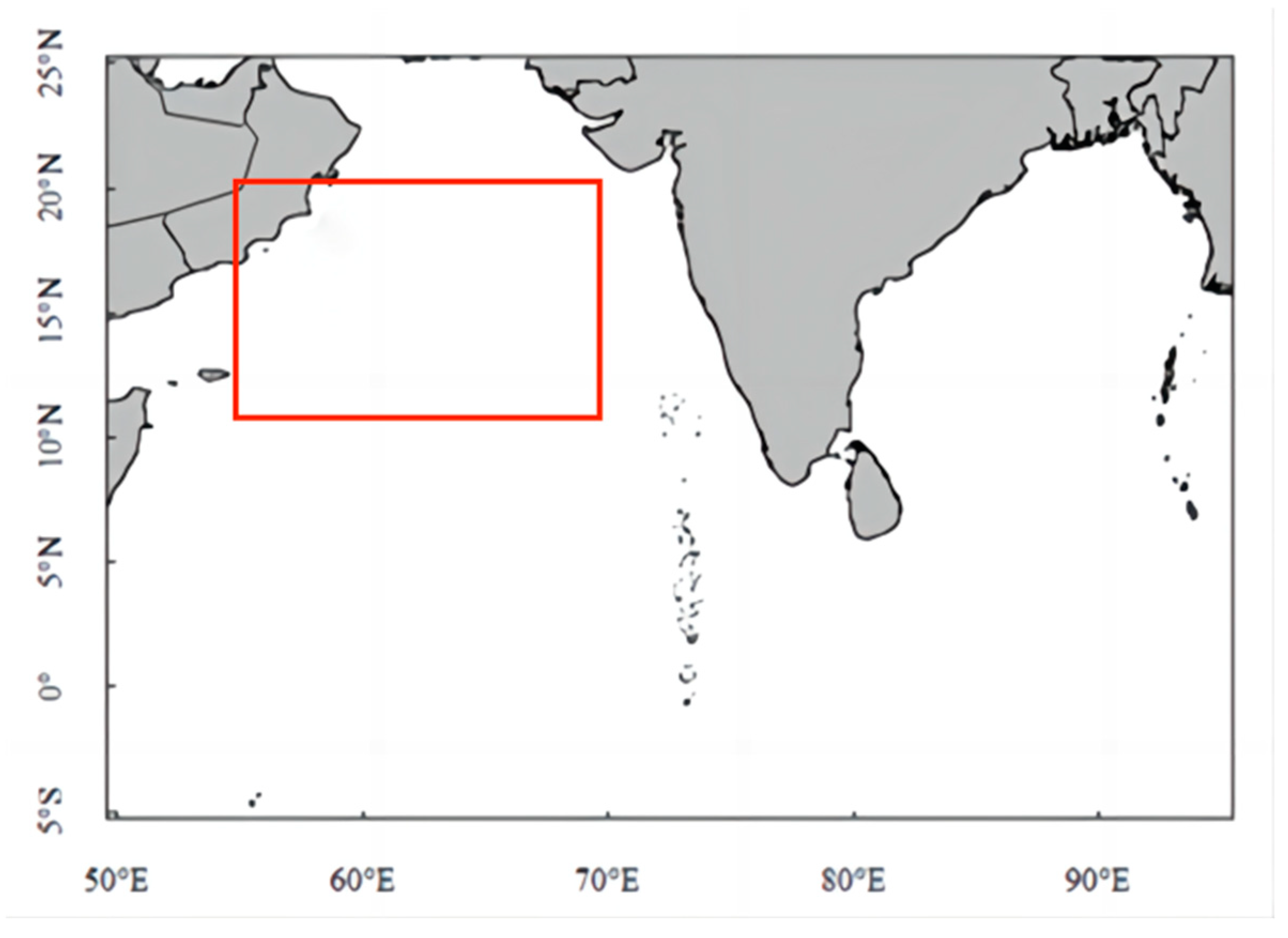
2.1. Material Source

The production statistics of S. oualaniensis in the northern Indian Ocean were obtained from the Squid Fishing Technology Group and High Seas Trawl Technology Group of the China Ocean Fisheries Association. Data were collected from 2017 to 2019, on a monthly basis, at a spatial resolution of 0.5 × 0.5°. The fishing ground analyzed in this study was mainly distributed in the waters between 10~20° N and 55~70° E in the northern Indian Ocean (Figure 1). The collected data included date, longitude, latitude, and the total catch.
According to the results of previous studies, the marine environmental factors that mainly affect the habitat distribution of S. oualaniensis in the Indian Ocean are SST, wind speed (WS), and PAR [7,10,11]. The above three factors were selected for inclusion in the model analysis, which included SST and PAR data from the National Ocean and Atmosphere Administration (NOAA) in (https://oceanwatch.pifsc.noaa.gov/erddap/index.html) (accessed on 15 July 2021), and WS from the Hawaii University (http://apdrc.soest.hawaili.edu/data/data.php) (accessed on 18 July 2021), on a monthly time scale and spatial resolution of 0.5 × 0.5°.

2.2. Analysis Method

2.2.1. Calculation

Catch per unit effort (CPUE) was used to quantify the density of S. oualaniensis. According to the main operation time, the fishery data from January to March and October to December were selected to calculate the catch and operation times in the range of 0.5 × 0.5°, and the CPUE was calculated as follows:
CPUE = C E
where CPUE is metric tons/times; C represents the output of a fishing boat in one day; E represents the corresponding number of operations. The environmental data and fishery data with a resolution of 0.5 × 0.5° were matched with the fishery data (time; latitude and longitude; production; CPUE) using Kriging interpolation. Using a semi-variogram, spatial interpolation was performed on three environmental factors with good predictive performance and the corresponding fishery data. In order to visualize the model output, the semivariogram was fitted using a Gaussian model in ArcGIS 10.3 so that the environmental and fishery data corresponded.

2.2.2. Single-Factor Suitability Index (SI) Model

A single-factor SI model was made with SST, WS, and PAR, using CPUE from January to March and from October to December in 2017–2018. The range of SI was from 0 to 1. When the CPUE in the region was maximum, SI equaled 1. When CPUE was 0, SI equaled 0 [18,19]. The SI model was established according to CPUE, as follows:
S I = C P U E i C P U E i , m i n C P U E i , m a x C P U E i , m i n
where CPUEi refers to the CPUE in the interval i; CPUEi,max refers to the maximum CPUE in the i range; CPUEi,min refers to the minimum CPUE in the i range.
The Statistical Package for the Social Sciences (SPSS) was used to fit SI values with different environmental factors (SST, WS, and PAR) as input values using the least-square method. The fitting formula is as follows:
SI X = exp [ a × ( X b ) 2 ]
where a and b are the model parameters estimated by the least-square method to minimize the residual difference between the observed and predicted values; and X is the value of the environment variable. The value of SIX ranges from 0 to 1.

2.2.3. Habitat Suitability Index (HSI) Model

Based on the established SI model of a single additional environmental factor, environmental factors were provided with different weights [13] (Table 1), integrated HSI models under different weighting schemes were established, and the optimum HSI model was selected through comparison and analysis. The HSI calculation formula is as follows:
HIS = kSST × SISST + kWS × SIWS + kPAR × SIPAR
where kSST, kWS, and kPAR are, respectively, the weight values of SI models of SST, WS, and PAR, while SISST, SIWS, and SIPAR are, respectively, the SI values of SST, WS, and PAR.

2.2.4. HSI Model Screening and Verification

According to the HSI models established above under different weights, the HSI values from January to March and October to December 2017–2018 were calculated ranging from 0 to 1. HSI ≤ 0.2, 0.2 < HSI < 0.6, and HSI ≥ 0.6, respectively, defined as unsuitable habitats, normal habitats, and suitable habitats for the northern Indian Ocean S. oualaniensis population [20,21], and the proportion of yield, fishing effort, and CPUE for the three types of habitats were calculated. By comprehensively comparing the proportion of yield and fishing effort and the CPUE value, the optimal weight scheme was selected to obtain the optimal HSI model. In particular, the larger the proportion of fishing effort and yield, the better the model prediction. Analogously, the larger the CPUE value over 0.6, the better the predictive ability of the model was. By comparing the corresponding stations with CPUE values and the distribution of fishing grounds obtained using the HSI model, the prediction accuracy of the HSI model was calculated with a bound of 0.6.
The 2019 data were used to verify the model, and were integrated into the HSI model to calculate the yield share, fishing effort share, and CPUE value of the three types of habitat [20,21]. Based on the comprehensive HSI model that was obtained, the HSI spatial distribution maps from January to March and from October to December in 2017, 2018, and 2019 were made and superimposed with the distribution of CPUE to verify the accuracy and feasibility of the model.

3. Results and Analysis

3.1. SI Model

The relationship between SI and environment variables fitted with the least-square method shows that when R2 is greater than 0.6 and closer to 1, the relationship between SI and environment variables is in line with normal distribution. When p is less than 0.01, there is a very significant relationship between SI and environmental variables, and when p is less than 0.05, there is a significant relationship. The research results show that the R2 of most SI models is >0.6, the model fitting effect is good, and the model fitting passes the significance test (p < 0.05), which means that these models can be used as HSI models (Table 2).

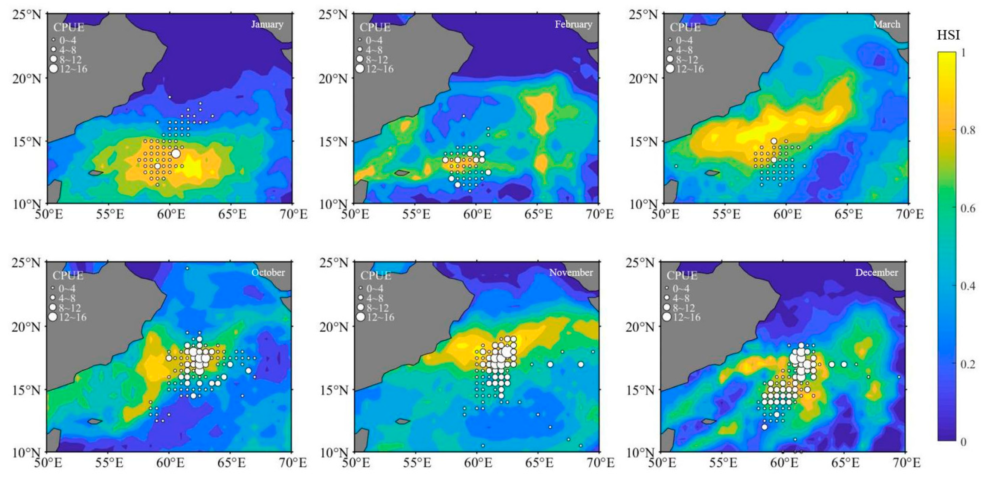
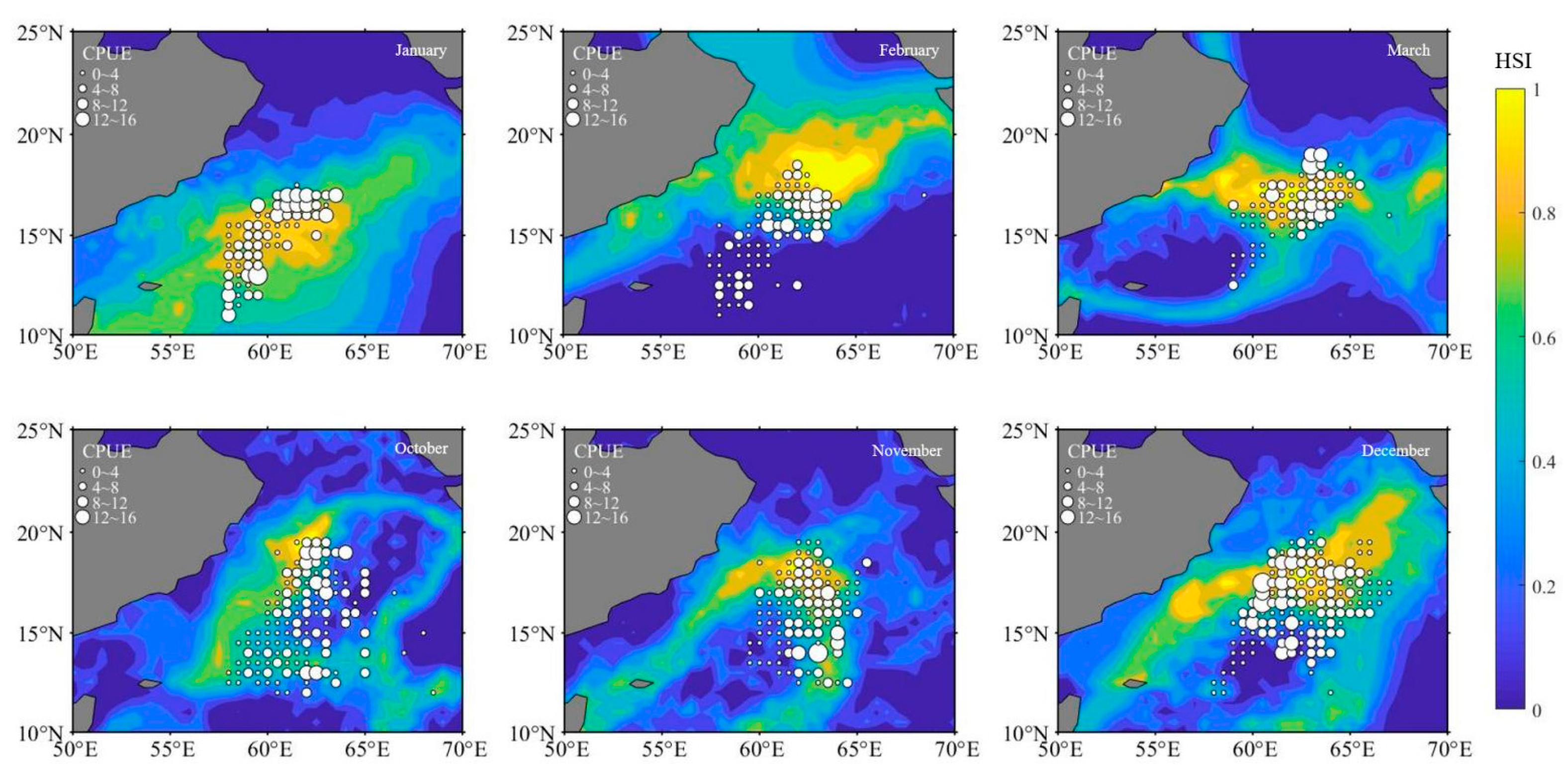
3.2. HSI Model Analysis

Since different environmental factors have different degrees of influence on the response variables, this paper compares and analyzes the optimal weight scheme and builds the optimal HSI model by assigning different weight ratios to the SI values of environmental factors. The yields, fishing effort, and CPUE ratio within the HSI interval (0~0.2; 0.2~0.6; 0.6~1) of each model were calculated. If the HSI interval of 0.6~1 accounted for more fishing effort, and the CPUE value increased in the interval, the prediction performance of the model was better. The results show that, among the different weight cases from 2017 to 2018, case 3 is most consistent with the larger proportion of fishing effort in the range from 0.6 to 1, and the CPUE value increases in the different HSI intervals (0~0.2; 0.2~0.6; 0.6~1). Therefore, case 3 is the optimal weight scheme. That is, the HSI model based on the weight of case 3 is the best HSI model, and the corresponding weight ratio of SST, WS, and PAR is 0.25:0.5:0.25. The environmental factor with the highest values was WS, followed by the equal weight ratio of SST and PAR (Table 3 and Table 4).

3.3. Model Verification and Screening Results

The optimal HSI model was established based on 2017–2018 data to predict the distribution of a suitable habitat for S. oualaniensis in the northern Indian Ocean in 2019, and the fishery data from that year were used for verification and screening. The fishery and environmental data of 2019 were brought into the HSI model based on weight case 3, and the yield, fishing effort ratio, and the CPUE values in different HSI intervals (0~0.2; 0.2~0.6; 0.6~1) were summarized (Table 1). The obtained results are shown in Table 5. The results showed that the yield and fishing effort ranged by more than 60% in the HSI range of 0.6~1 in January to March and October to December, and more than 80% in March, October, and November. The CPUE value increases in different HSI ranges [0, 0.2], [0.2, 0.6], [0.6, 1,0]. The CPUE values for 2017–2018, when the model was built (Figure 2), and for 2019, when the forecast was made (Figure 3), are mostly concentrated in the higher HSI value range. These results indicate that the HSI model can best evaluate and predict the habitat status for S. oualaniensis in the northern Indian Ocean, and the SI value of WS is the largest proportion of the total weight during the model’s construction. The results show that WS exerts the main influence on the distribution of a suitable habitat for S. oualaniensis in the northern Indian Ocean.

4. Discussion

4.1. Effects of Environmental Factors on the Spatial Distribution of the Habitat of S. oualaniensis

As a cephalopod with a short life cycle, the pelagic habitat of S. oualaniensis is defined within narrow boundaries in terms of environmental variables, and is also sensible to closely related factors [22,23]. Studies have shown that changes in SST, SSH, SSS, chl-a, primary productivity, and other environmental factors will cause changes in the habitat selection of S. oualaniensis [7,24].
The northern Indian Ocean is affected by monsoon throughout the year. Monsoon is one of the most important factors driving environmental change and ecological processes in the northern Indian Ocean. Monsoon directly affects various hydrological factors, especially the spatial distribution and temporal changes in water flow direction, velocity, temperature, salinity, and sea surface nutrients [25]. The monsoon blows onto the water, causing it to drift with the wind and provoking the upwelling of nutrients from the deep layers to the illuminated surface of the water column, thereby promoting primary production [26] and ultimately driving the spatial distribution of S. oualaniensis [27]. S. oualaniensis is a warm ocean species, and SST has a direct impact on its growth, reproduction, and migration, as well as being one of the main factors causing its spatial distribution [28,29]. Many scholars have studied the relationship between the marine environment and the distribution of S. oualaniensis. For example, Chen and Ye [2] concluded that sea surface temperature played an important role in the formation of core fishing areas, with an appropriate sea surface temperature between 16.4 and 29.0 °C. Yu and Chen [24] combined four environmental factors, namely, SST, SSS, SSH, and chl-a, and found that SST was a major factor affecting S. oualaniensis’ spatial distribution in the South China Sea. According to the habitat suitability index model, combined with CPUE, Zhou et al. [30] proved that SST is a factor significantly affecting the habitat of S. oualaniensis in the South China Sea. Changes in climate and marine environment will modify the quantity and distribution of marine phytoplankton. When the PAR value increases, the quantity of marine phytoplankton will increase correspondingly, thus increasing marine primary productivity and food resources for zooplankton species. Therefore, the increase in PAR is conducive to food provision in S. oualaniensis, affecting its distribution and the fishing effort in the northern Indian Ocean [31,32,33]. In addition, as an important link in the marine food chain and food web, the distribution of S. oualaniensis is influenced by changes in its prey and predator distributions and abundances, as well as environmental factors.

4.2. Analysis of Habitat Suitability Index Model of S. oualaniensis

Using the optimal weight ratio scheme, it was found that the weight contribution rate of the wind speed was the largest, while the contribution rate of sea surface temperature and photosynthetically active radiation were similar. The largest contribution rate of wind speed may be due to the overriding influence of monsoon, which has an impact on the suitable habitat index [25,26,27]. The monsoon substantially drives the climate in the Indian Ocean. From April to June each year, the Southwest Monsoon starts, the Somali Sea flows strongly, and the subsurface cold water come to the surface. With the outbreak of the Southwest Monsoon and the strengthening of evaporation, the combined effects of the two factors lead to a sharp cooling of the water temperature in the North Indian Ocean, including the Arabian Sea, thereby affecting the habitat distribution of S. oualaniensis. In addition, monsoons cause changes in ocean currents, affecting habitat suitability. The model was cross-validated using a distinct dataset from 2019. According to the prediction results of the HSI model of Indian Ocean S. oualaniensis in 2019, it was found that when the fishing effort was taken as the index, the results were better in January, March, October, and November, and the fishing efforts in the appropriate habitat accounted for a relatively high proportion of the total results, all of which were above 70%. The results in February and December were poor, and the fishing efforts in suitable habitats accounted for more than 60% of the total, which was lower than that in other months. At the same time, according to the superimposed map of habitat suitability index and CPUE value in 2019, the distribution range of suitable habitat for northern Indian Ocean S. oualaniensis was roughly 12~18° N and 55~65° E. This is also the main distribution area indicated by scholars studying the central fishing ground for S. oualaniensis in the northern Indian Ocean [34,35]. The range of suitable habitat in February was concentrated in the north. By calculating the prediction accuracy of the HSI model and the corresponding sea area CPUE, a gap was found in the prediction accuracy in February compared to other months. The bias in the February forecast may be due to the influence of additional environmental factors or the inaccurate weighting of the environmental factors that were considered environmental weights, resulting in a lower suitable habitat index for areas where fishing efforts were carried out.
According to the generated maps of spatial distribution of S. oualaniensis, the HSI model fits well with S. oualaniensis CPUEs. Future HSI models should consider additional factors and also incorporate the effects of climate change to further enhance the forecast of S. oualaniensis fishery forecast.

5. Conclusions

According to fishery and environmental data from 2017 to 2018, an HSI model was established based on the established single-factor SI model, and different environmental factors were weighted. Based on the HSI of the fishery data of S. oualaniensis fisheries in the Indian Ocean and environmental factors such as SST, WS, and PAR, it was found that the weight contribution of the wind speed was the largest. In addition, S. oualaniensis is influenced by various other environmental factors, like PAR, which affects the abundance of plankton and, hence, the spatial and temporal distribution of the S. oualaniensis fishery in the northern Indian Ocean. The abundance of plankton and other food resources is conducive to the growth and feeding of the S. oualaniensis, which, in turn, affects the distribution of its bait organisms and has a potential impact on the resource quantity and spatiotemporal distribution of S. oualaniensis fisheries in the northern Indian Ocean. The here-presented HSI model could better reflect the habitat distribution of S. oualaniensis in the northern Indian Ocean.
This study selected three environmental factors, SST, WS, and PAR, to construct an HSI model. However, the actual growth environment of S. oualaniensis is also affected by various other environmental factors. A more comprehensive analysis of the impact of each environmental factor on the habitat is needed to make the HSI model more accurate.
In the future, it is necessary to strengthen the collection of time series samples, improve the quality of fishing data, comprehensively consider more environmental factors and climate events, and accurately analyze the changes in the fishing grounds and habitats, which could provide a basis for the rational development of the fishery and the establishment of relevant fishing situation prediction models.

Author Contributions

J.Y., L.W. and S.L. contributed to the generation of research ideas and writing the essay. H.Z. and Z.F. acquired and analyzed data and revised the paper, guiding the writing and ideas. All authors have read and agreed to the published version of the manuscript.

Funding

This work was funded by the National Key R&D Program of China (2019YFD0901404), National Nature Foundation of China (NSFC41876141), and sponsored by the Natural Science Foundation of Shanghai (18ZR1449800) and Funding for the Opening of Key Laboratories for Offshore Fishery Development by the Ministry of Agriculture (LOF 2021-01).

Institutional Review Board Statement

The article only uses the production data of S. oualaniensis caught by Chinese legal fleets in the northwest Indian Ocean, and does not use the biological data of squid. The production data were taken with the permission from the Shanghai Ocean University, which is in charge of oceanic fisheries research in China. We confirm that the fisheries from which the squid were obtained were conducted by a legitimate Chinese company with appropriate permits to fish in the waters described in the paper. We also confirm that none of the squid was collected for the purpose of this study. They were caught as fisheries catch.

Data Availability Statement

The data presented in this study are available on request from the corresponding author.

Acknowledgments

We acknowledge the support of the captains and crews of the commercial jigging vessels recruited for scientific surveys.

Conflicts of Interest

The authors declare no conflicts of interest.

References

  1. Dong, Z.Z. Biology of Oceanic Economic Cephalopod in the World; Shandong Science and Technology Press: Jinan, China, 1991; pp. 91–94. [Google Scholar]
  2. Chen, X.J.; Ye, X.C. Preliminary study on the relationship between fishing ground of Sthenoteuthis oualaniensis and environmental factors in northwestern Indian Ocean. J. Shanghai Fish. Univ. 2005, 14, 55–60. [Google Scholar] [CrossRef]
  3. Voss, G.L. Cephalopod resources of the world. FAO Fish Circ. 1973, 10, 75. [Google Scholar]
  4. Chen, X.J.; Liu, B.L.; Wang, Y.G. Cephalopods of the World; China Ocean Press: Beijing, China, 2009; pp. 312–442. [Google Scholar]
  5. Vecchione, M. Extraordinary abundance of squid paralarvae in the tropical eastern Pacific Ocean during El Niño of 1987. Fish. Bull. 1999, 97, 1025–1030. [Google Scholar]
  6. Sajikumar, K.K.; Ragesh, N.; Venkatesan, V.; Koya, K.P.; Sasikumar, G.; Kripa, V.; Mohamed, K.S. Morphological development and distribution of paralarvae and juveniles of purpleback flying squid Sthenoteuthis oualaniensis (Ommastrephidae), in South-eastern Arabian Sea. Vie Milieu-Life Environ. 2018, 68, 75–86. [Google Scholar]
  7. Chen, X.J.; Shao, F. Study on the Resource Characteristics of Sthenoteuthis oualaniensis and Their Relationships with the Sea Conditions in the High Sea of the Northwestern Indian Ocean. Period. Ocean Univ. China 2006, 36, 611–616. [Google Scholar]
  8. Schott, F.A.; McCreary, J.P., Jr. The monsoon circulation of the Indian Ocean. Prog. Oceanogr. 2001, 51, 1–123. [Google Scholar] [CrossRef]
  9. Schott, F.A.; Xie, S.P.; Mccreary, J.P. Indian Ocean circulation and climate variability. Rev. Geophys. 2009, 47, 549. [Google Scholar] [CrossRef]
  10. Roxy, M.K.; Ritika, K.; Terray, P.; Murtugudde, R.; Ashok, K.; Goswami, B.N. Drying of Indian subcontinent by rapid Indian Ocean warming and a weakening land sea thermal gradient. Nat. Commun. 2015, 6, 7423. [Google Scholar] [CrossRef] [PubMed]
  11. Wen, L.; Zhang, H.; Fang, Z.; Chen, X. Preliminary standardization of Sthenoteuthis oualaniensis in Northern Indian Ocean. Trans. Oceanol. Limnol. 2022, 44, 89–97. [Google Scholar]
  12. US Fish and Wildlife Service. 101ESM Habitat as a Base for Environmental Assessment; Division of Ecological: Washington, DC, USA, 1980.
  13. Yu, W.; Guo, A.; Zhang, Y.; Chen, X.; Qian, W.; Li, Y. Climate-induced habitat suitability variations of chub mackerel Scomber japonicus in the East China Sea. Fish. Res. 2018, 207, 63–73. [Google Scholar] [CrossRef]
  14. Feng, Z.P.; Yu, W.; Chen, X.J.; Liu, B.L.; Zhang, Z. Analysis of fishing ground of jumbo flying squid Dosidicus gigas in the southeast Pacific Ocean off Peru based on weighting-based habitat suitability index model. J. Shanghai Ocean Univ. 2021, 29, 878–888. [Google Scholar]
  15. Gong, C.X.; Chen, X.J.; Gao, F.; Guan, W.J.; Lei, L. Review on habitat suitability index in fishery science. J. Shanghai Ocean Univ. 2011, 20, 260–269. [Google Scholar]
  16. Liu, H.W.; Yu, W.; Chen, X.J.; Zhu, W.B. Construction of habitat suitability index model for Illex argentinus based on vertical water temperature at different depths. J. Dalian Ocean Univ. 2021, 36, 1035–1043. [Google Scholar]
  17. Wang, Y.F.; Chen, X.J. Comparisons of habitat suitability index models of skipjack tuna in the Western and Central Pacific Ocean. J. Shanghai Ocean Univ. 2017, 26, 743–750. [Google Scholar]
  18. Mohri, M. Seasonal changes in Bigeye tuna fishing areas in relation to the oceanographic parameters in the Indian Ocean. J. Natl. Fish. Univ. 1999, 47, 43–54. [Google Scholar]
  19. Fang, X.Y.; Chen, X.J.; Ding, Q. Optimization Fishing Ground Prediction Models of Dosidicus gigas in the High Sea off Chile Based on Habitat Suitability Index. J. Guangdong Ocean Univ. 2014, 34, 67–73. [Google Scholar]
  20. Yu, W.; Yi, Q.; Chen, X.; Chen, Y. Modelling the effects of climate variability on habitat suitability of jumbo flying squid, Dosidicus gigas, in the Southeast Pacific Ocean off Peru. ICES J. Mar. Sci. 2016, 73, 239–249. [Google Scholar] [CrossRef]
  21. Yu, W.; Chen, X.J.; Zhang, Y. Seasonal habitat patterns of jumbo flying squid Dosidicus gigas off Peruvian waters. J. Mar. Syst. 2019, 194, 41–51. [Google Scholar] [CrossRef]
  22. Ichii, T.; Mahapatra, K.; Sakai, M.; Wakabayashi, T.; Okamura, H.; Igarashi, H.; Inagake, D.; Okada, Y. Changes in abundance of the neon flying squid Ommastrephes bartramii in relation to climate change in the central North Pacific Ocean. Mar. Ecol. Prog. Ser. 2011, 441, 151–164. [Google Scholar] [CrossRef]
  23. Alabia, I.D.; Saitoh, S.I.; Igarashi, H.; Ishikawa, Y.; Usui, N.; Kamachi, M.; Awaji, T.; Seito, M. Future projected impacts of ocean warming to potential squid habitat in western and central North Pacific. ICES J. Mar. Sci. 2016, 73, 1343–1356. [Google Scholar] [CrossRef]
  24. Yu, W.; Chen, X.J. Analysis on Habitat Suitability Index of Sthenoteuthis oualaniensis in Northwestern Indian Ocean from September to October. J. Guangdong Ocean Univ. 2012, 32, 74–80. [Google Scholar]
  25. Hood, R.R.; Beckley, L.E.; Wiggert, J.D. Biogeochemical and Ecological Impacts of Boundary Currents in the Indian Ocean. Prog. Oceanogr. 2017, 156, 290–325. [Google Scholar] [CrossRef]
  26. Wiggert, J.D.; Jones, B.H.; Dickey, T.D.; Brink, K.H.; Weller, R.A.; Marra, J.; Codispoti, L.A. The northeast monsoon’s impact on mixing, phytoplankton biomass and nutrient cycling in the Arabian Sea. Deep Sea Res. Part II Top. Stud. Oceanogr. 2000, 47, 1353–1385. [Google Scholar] [CrossRef]
  27. Hastenrath, S. Regional Circulation Systems. Clim. Dyn. Trop. 1991, 8, 114–218. [Google Scholar]
  28. Sims, D.W.; Genner, M.J.; Southward, A.J.; Hawkins, S.J. Timing of squid migration reflects North Atlantic climate variability. Proc. R. Soc. B Biol. Sci. 2001, 268, 2607–2611. [Google Scholar] [CrossRef] [PubMed]
  29. Caballero-Alfonso, A.M.; Ganzedo, U.; Trujillo-Santana, A.; Polanco, J.; del Pino, A.S.; Ibarra-Berastegi, G.; Castro-Hernández, J.J. The role of climatic variability on the short term fluctuations of octopus captures at the Canary Islands. Fish. Res. 2010, 102, 258–265. [Google Scholar] [CrossRef]
  30. Zhou, W.F.; Xu, H.Y.; Li, A.Z.; Cui, X.S.; Chen, G.B. Comparison of habitat suitability index models for purpleback flying squid (Sthenoteuthis oualaniensis) in the open South China sea. Appl. Ecol. Environ. Res. 2019, 17, 4903–4913. [Google Scholar] [CrossRef]
  31. Trotsenko, B.G.; Pinchukov, M.A. Mesoscale distribution features of the purpleblack squid Sthenoteuthis Ouslsniensis with reference to the structure of the upper quasi homogeneous layer in the western India Ocean. Oceanology 1994, 34, 380–385. [Google Scholar]
  32. Yang, X.M.; Chen, X.J.; Zhou, Y.Q.; Tian, S.Q. A marine remote sensing-based preliminary analysis on the fishing ground of purple flying squid Sthenoteuthis oualaniensis in the northwest Indian Ocean. J. Shanghai Fish. Univ. 2006, 30, 669–675. [Google Scholar]
  33. Qian, M.; Gong, J.; Fan, J.; Yu, W.; Chen, X.; Qian, W. Variations in the abundance and spatial distribution of Ommastrephes bartramii in the Northwest Pacific Ocean based on photosynthetic active radiation. Acta Oceanol. Sin. 2020, 42, 44–53. [Google Scholar]
  34. Lu, H.J.; Ou, Y.Z.; He, J.R.; Zhao, M.L.; Chen, Z.Y.; Chen, X.J. Age, growth and population structure analyses of the purpleback flying squid Sthenoteuthis oualaniensis in the Northwest Indian Ocean by beak microstructure. J. Mar. Sci. Eng. 2022, 10, 1094. [Google Scholar] [CrossRef]
  35. Jeena, N.S.; Sajikumar, K.K.; Rahuman, S.; Ragesh, N.; Koya, K.S.; Chinnadurai, S.; Sasikumar, G.; Mohamed, K.S. Insights into the divergent evolution of the oceanic squid Sthenoteuthis oualaniensis (Cephalopoda: Ommastrephidae) from the Indian Ocean. Integr. Zool. 2023, 18, 924–948. [Google Scholar] [CrossRef] [PubMed]
Figure 1. Research scope of the squid Sthenoteuthis oualaniensis in the Indian Ocean. The red box represents the fishing operation area for data used by the research institute.
Fishes 09 00107 g001
Figure 2. The spatial distribution of CPUE overlapped with the HSI values in 2017–2018. The larger the CPUE coverage, the higher the overlap with the HSI values.
Fishes 09 00107 g002
Figure 3. The spatial distribution of CPUE overlapped with the HSI values from 2019, calculated by the optimal model. The larger the CPUE coverage, the more it overlaps with the predicted habitat.
Fishes 09 00107 g003
Table 1. Different scenarios for the weights of different environmental factors.
ScenarioskSSTkWSkPAR
Case10.50.250.25
Case20.3330.3330.333
Case30.250.50.25
Case40.250.250.5
Case50.10.10.8
Case60.10.80.1
Case7001
Case8010
Table 2. Fitting formula of SI models. The closer R2 is to 1, the more significant the impact of environmental factors.
Environmental FactorsMonthSI ModelR2p
SSTJanuarySISST = exp [−4.012 × (XSST − 25.877)2]0.9810.006
FebruarySISST = exp [−7.845 × (XSST − 25.498)2]0.9820.001
MarchSISST = exp [−11.417 × (XSST − 26.756)2]0.9990.008
OctoberSISST = exp [−4.696 × (XSST − 28.089)2]0.9970.001
NovemberSISST = exp [−7.814 × (XSST − 27.889)2]0.7600.018
DecemberSISST = exp [−6.75 × (XSST − 26.459)2]0.9250.001
WSJanuarySIWS = exp [−0.919 × (XWS − 6.926)2]0.7470.001
FebruarySIWS = exp [−14.23 × (XWS − 5.229)2]0.5490.005
MarchSIWS = exp [−1.896 × (XWS − 4.035)2]0.6890.031
OctoberSIWS = exp [−9.212 × (XWS − 3.264)2]0.9550.001
NovemberSIWS = exp [−1.029 × (XWS − 4.987)2]0.6230.017
DecemberSIWS = exp [−4.895 × (XWS − 7.45)2]0.8260.016
PARJanuarySIPAR = exp [−0.564 × (XPAR − 43.059)2]0.7420.003
FebruarySIPAR = exp [−0.501 × (XPAR − 48.204)2]0.5360.009
MarchSIPAR = exp [−1.061 × (XPAR − 54.238)2]0.8140.001
OctoberSIPAR = exp [−6.686 × (XPAR − 47.041)2]0.7560.001
NovemberSIPAR = exp [−0.547 × (XPAR − 41.682)2]0.7330.001
DecemberSIPAR = exp [−1.552 × (XPAR − 39.563)2]0.6130.001
Table 3. Percentage of catch and effort under different HSI class intervals sourced from different weighting models during 2017–2018.
MonthHSICase1Case2Case3Case4
Catch/%Effort/%Catch/%Effort/%Catch/%Effort/%Catch/%Effort/%
January[0–0.2]0.21 1.73 0.16 1.64 0.15 1.51 0.18 1.68
(0.2–0.6)36.98 39.76 24.17 28.86 17.97 22.21 37.46 36.97
[0.6–1]62.82 58.51 75.67 69.50 81.88 76.29 62.36 61.35
February[0–0.2]2.65 1.74 2.76 1.39 3.24 2.44 0.60 0.60
(0.2–0.6)29.97 23.28 42.50 44.78 38.81 46.24 47.46 38.36
[0.6–1]67.38 74.98 54.74 53.83 57.95 51.32 51.94 61.04
March[0–0.2]0.00 0.00 0.00 0.00 0.00 0.00 0.00 0.00
(0.2–0.6)29.85 25.16 11.27 13.57 8.53 14.50 36.51 32.96
[0.6–1]70.15 74.84 88.73 86.43 91.47 85.50 63.49 67.04
October[0–0.2]3.56 3.38 1.84 2.06 6.77 7.60 7.85 8.74
(0.2–0.6)38.91 43.70 40.62 45.02 43.33 41.68 46.20 51.95
[0.6–1]57.53 52.92 57.53 52.92 49.90 50.72 45.95 39.31
November[0–0.2]5.69 10.68 0.76 2.73 0.85 3.13 0.85 3.09
(0.2–0.6)19.66 20.17 35.93 40.22 36.05 40.22 23.84 30.55
[0.6–1]74.64 69.16 63.31 57.05 63.10 56.65 75.26 66.32
December[0–0.2]5.03 5.75 2.85 3.77 4.28 5.40 3.75 4.39
(0.2–0.6)55.44 57.08 55.69 58.01 44.04 46.85 59.82 59.68
[0.6–1]39.53 37.17 41.46 38.22 51.68 47.74 36.43 35.93
MonthHSICase5Case6Case7Case8
Catch/%Effort/%Catch/%Effort/%Catch/%Effort/%Catch/%Effort/%
January[0–0.2]6.20 9.04 1.14 5.59 10.28 12.06 1.95 6.91
(0.2–0.6)32.69 32.89 18.96 22.70 33.57 30.85 8.71 13.74
[0.6–1]61.10 58.07 79.90 71.72 56.16 57.09 89.35 79.34
February[0–0.2]1.83 0.90 37.82 46.87 17.47 11.89 42.05 53.68
(0.2–0.6)42.01 28.51 4.23 6.82 22.97 15.22 0.00 0.00
[0.6–1]56.16 70.60 57.95 46.32 59.56 72.89 57.95 46.32
March[0–0.2]7.84 6.69 0.00 0.00 24.38 15.56 0.00 0.00
(0.2–0.6)38.69 35.55 9.24 19.44 29.18 36.93 9.20 19.25
[0.6–1]53.46 57.76 90.76 80.56 46.44 47.51 90.80 80.75
October[0–0.2]32.71 41.85 14.69 19.72 36.65 45.76 19.05 25.73
(0.2–0.6)17.23 14.54 31.57 25.65 13.30 10.63 27.20 19.63
[0.6–1]50.05 43.61 53.74 54.63 50.05 43.61 53.75 54.64
November[0–0.2]1.21 3.70 1.43 4.10 13.63 17.76 1.50 4.92
(0.2–0.6)34.03 34.04 10.58 15.92 21.12 19.23 10.44 14.81
[0.6–1]64.76 62.26 87.99 79.98 65.25 63.01 88.06 80.27
December[0–0.2]34.76 31.45 27.22 29.28 41.91 40.71 26.8428.77
(0.2–0.6)23.57 24.38 8.28 11.59 7.16 7.43 7.8211.63
[0.6–1]41.67 44.17 64.50 59.14 50.93 51.87 65.3459.6
Table 4. CPUE under different HSI class intervals sourced from different weighting models during 2017–2018.
MonthHSICPUE (t/time)
Case1Case2Case3Case4Case5Case6Case7Case8
January[0–0.2]0.52 0.26 0.25 0.40 1.58 0.94 1.75 0.99
(0.2–0.6)2.11 1.88 1.82 2.00 1.98 2.05 2.09 1.95
[0.6–1]2.82 3.06 2.93 2.99 3.08 2.87 2.82 2.94
February[0–0.2]3.18 4.42 2.23 2.57 6.59 1.65 5.12 1.90
(0.2–0.6)2.66 2.16 1.87 2.46 4.07 3.69 4.17 0.00
[0.6–1]2.29 2.86 3.79 2.39 1.68 3.79 1.78 3.79
March[0–0.2]0.00 0.00 0.00 0.00 2.01 0.00 2.61 0.00
(0.2–0.6)2.52 2.07 1.93 2.23 2.37 1.61 1.98 1.70
[0.6–1]2.04 2.23 2.28 2.17 2.07 2.32 2.18 2.29
October[0–0.2]5.46 5.20 5.36 5.43 5.23 5.29 5.28 5.33
(0.2–0.6)5.38 5.42 5.50 5.46 6.52 5.97 6.72 6.00
[0.6–1]7.40 7.40 6.74 7.31 6.91 6.28 6.91 6.28
November[0–0.2]4.10 2.89 2.68 2.33 3.92 3.71 4.97 3.25
(0.2–0.6)5.78 5.86 5.87 5.52 6.21 5.45 6.70 5.91
[0.6–1]7.92 7.67 7.97 7.81 7.23 7.89 6.97 7.81
December[0–0.2]5.17 4.81 4.88 5.10 6.51 5.39 6.58 5.36
(0.2–0.6)5.94 5.75 5.65 5.93 5.81 5.51 4.80 4.87
[0.6–1]6.16 7.13 7.14 6.16 5.10 6.65 5.25 6.78
Table 5. Forecast results of the S. oualaniensis HSI model in the Indian Ocean for 2019.
MonthHSICatch/%Effort/%CPUEPrediction Accuracy
[0–0.2]0.020.02 4.03100.00%
January(0.2–0.6)27.4118.015.12
[0.6–1]72.5781.975.83
[0–0.2]6.156.97 3.8356.82%
February(0.2–0.6)28.1528.544.01
[0.6–1]65.7064.49 5.40
[0–0.2]2.12 3.714.34 93.51%
March(0.2–0.6)8.83 8.474.84
[0.6–1]89.0587.824.86
[0–0.2]0.31 0.32 3.86 80.80%
October(0.2–0.6)13.45 18.52 4.12
[0.6–1]86.2481.164.54
[0–0.2]0.44 0.573.13 83.65%
November(0.2–0.6)15.39 20.86 3.60
[0.6–1]84.1778.574.42
[0–0.2]1.763.363.53 100.00%
December(0.2–0.6)34.2434.72 4.45
[0.6–1]64.00 61.92 5.00
Disclaimer/Publisher’s Note: The statements, opinions and data contained in all publications are solely those of the individual author(s) and contributor(s) and not of MDPI and/or the editor(s). MDPI and/or the editor(s) disclaim responsibility for any injury to people or property resulting from any ideas, methods, instructions or products referred to in the content.

