1. Introduction
Fish species classification is an important task for biologists and marine ecologists that is used frequently to estimate the relative abundance of fish species in their natural habitats and to monitor changes in their populations [
1]. The
Rastrelliger genus is classified within the family Scombridae, comprising epipelagic fish species predominantly inhabiting tropical and subtropical regions. Within the
Rastrelliger genus, three distinct species are identified:
R. brachysoma (Short mackerel),
R. kanagurta (Indian mackerel), and
R. faughni (Island mackerel). Notably, the Short mackerel and Indian mackerel have substantial economic importance within the Gulf of Thailand. Nevertheless, their populations have experienced significant declines due to extensive annual harvesting activities [
2,
3]. Recent data from the Food and Agriculture Organization of the United Nations (FAO) for 2019 highlighted the pivotal role of
R. brachysoma and
R. kanagurta in the global fisheries industry, as they were among the 70 principal species with capture production exceeding 150,000 t [
4]. Nonetheless, these fish belong to the same genus and display nearly identical morphologies, with shared features such as a streamlined body, blue–green coloration, and similar fin structures. These commonalities present difficulties in differentiating between them. Currently, distinguishing between these two species relies on manuals or the expertise of individuals. Traditional methods used for fish species classification are laborious, time-consuming, and expensive [
1]. These limitations pose challenges for consumers and academics unfamiliar with these fish. Additionally, from a consumer perspective,
R. brachysoma is priced higher than
R. kanagurta.
Morphology-based fish species classification is not only an error-prone process but also time-consuming. Given the vast number of fish species and their often-close resemblance to each other, relying solely on external characteristics makes classification a challenging task [
5]. Accurate fish classification, however, holds great importance from various aspects, such as yield forecasting, production management, and ecosystem monitoring [
6]. To address these fish classification challenges, a multitude of machine learning (ML) and deep learning (DL) approaches have been explored. ML methods, including decision trees, random forests, and support vector machines, have demonstrated satisfactory performance in image processing [
7,
8]. However, conventional ML heavily relies on iterative processes and human experience [
9]. In contrast, DL offers a fundamental advantage through its automatic hierarchical feature extraction process in image processing. In particular, the use of DL in machine vision systems for decision-making has gained popularity. Consequently, DL models are known for their ability to effectively handle raw data without the need for trial-and-error-based, hand-crafted, feature-extraction processes [
8]. DL has become an increasingly important tool in data analysis, being applied in various models and for various specific proposes, with the models becoming more and more efficient, especially in the context of utilizing transfer learning techniques with pre-trained models. Transfer learning is a machine learning technique where a model trained on one task is reused or adapted as a starting point for a second, related task. Such techniques can offer several advantages over traditional methods, potentially making this approach more effective than other approaches, such as by substantially reducing the need for species-specific training data. Pre-trained models can already learn low-level features, such as edges and textures, applicable to various image classification tasks. This “feature extraction” capability can be transferred to the specific task of differentiating, reducing training time. Moreover, transfer learning has emerged as a valuable technique for fine-tuning deep neural network structures, enhancing their ability to discern relevant information effectively. In the realm of DL models commonly employed in image processing for fish classification, notable options include the convolutional neural network (CNN), visual geometry group (VGG), residual neural network (ResNet), krizhevsky neural network (AlexNet), efficient convolutional neural networks for mobile vision applications (MobileNet), and depthwise separable convolutions or extreme inception (Xception). These models offer diverse capabilities and have been instrumental in advancing the field of fish species identification.
For example, ref. [
10] used ResNet-50 to classify coral texture images, achieving an outstanding accuracy rate surpassing 95.87%. However, accurate image classification remains challenging, especially with limited sample sizes. Rauf et al. [
5] introduced the Fish-Pak dataset with 915 images across six classes and utilized a 32-layer VGG architecture, achieving an impressive 87.33% accuracy in fish species classification. In another study, Iqbal et al. [
11] utilized a variant of AlexNet, comprising four convolutional layers and two fully connected layers, to classify 468 fish categories, achieving a notable accuracy rate of 90.48%. Carnagie et al. [
12] used the Xception model to classify essential oil plants, reporting highest accuracy levels of 75% during validation and 81% during testing by the fourth epoch. Furthermore, Akgül et al. [
13] utilized Xception for fish freshness detection and obtained successful outcomes when combined with Yolo-v5, achieving 88.00% and 94.67% accuracy levels for anchovy (
Engraulis encrasicolus) and Horse mackerel (
Trachurus trachurus) datasets, respectively. Chen et al. [
14] employed a deep neural system for fish classification, utilizing two branches: one for detecting, aligning, and classifying fish based on pose and scale variations; and the other for leveraging contextual information to infer fish types. Asli et al. [
15] introduced a method involving two-dimensional Zernike polynomials for image classification. Mathur and Goel [
16] applied the ResNet-50 network for underwater fish classification, achieving improved accuracy despite limited datasets, while Lu and Honarvar Shakibaei Asli [
17] utilized Gaussian filter preprocessing, U-net segmentation, and ResNet-50/Inception-v3 classification for the analysis of specific data.
Applying DL for classifying the species of mackerel, Kurniawan et al. [
18] utilized a CNN to classify images of
R. brachysoma and
R. kanagurta. Their results revealed a model accuracy of 100% for training and 92.60% for validation, with 94.70% testing accuracy. However, they exclusively utilized female
R. brachysoma and male
R. kanagurta as samples.
Most of the published studies required transporting fish samples to the laboratory and capturing images in controlled environments, such as using cameras inside light-controlled boxes, with specific guidelines. In today’s context, where nearly everyone uses mobile phones for communication and photography, if it were possible to capture images using mobile phones directly at the sampling site and to subsequently use these images to differentiate between variations, this would certainly streamline such fisheries work. This approach might even lead to the development of applications for more accurate fish species differentiation in the future, especially those within the same genus that display very similar physical characteristics.
The objective of the current study was to utilize transfer learning models and to apply pre-trained models (RestNet50, Xception, InceptionV3, VGG19, VGG16, and MobileNetV3Small). These models were used to classify images of the R. brachysoma and R. kanagurta fish species, captured using smartphones. Additionally, the best-performing model was fine-tuned by increasing the number of epochs to achieve optimal predictive performance.
2. Materials and Methods
2.1. Data Collection
Samples of fresh adult-sized mackerel, with lengths of 15–20 cm, were obtained from five fishing zones: Zone 1, Eastern Gulf of Thailand; Zone 2, Inner Gulf of Thailand; Zone 3, Western Gulf of Thailand (Upper); Zone 4, Western Gulf of Thailand (Lower); and Zone 6, Andaman Sea (Upper). Collections were conducted six times within a year in December 2021 and in January, March, May, July, and September 2022. In total, 517 samples were collected, comprising 267 samples of R. brachysoma and 250 samples of R. kanagurta. The samples were transported under cold conditions using ice and an insulated container to the Faculty of Fisheries, Kasetsart University, Bangkok, Thailand, where image processing was conducted. The implementation of all programming codes was carried out using Python within Google Colab.
2.2. Image Acquisition
Each fish was manually identified to the species level by an expert and then smartphones (Xiaomi Mi 9, Xiaomi technology (Thailand) limited, Bangkok, Thailand) equipped with a 48 Mp/8000 × 6000 Mp camera were used to capture images of each fish (see
Table 1 for details) and transmitted for the processing process.
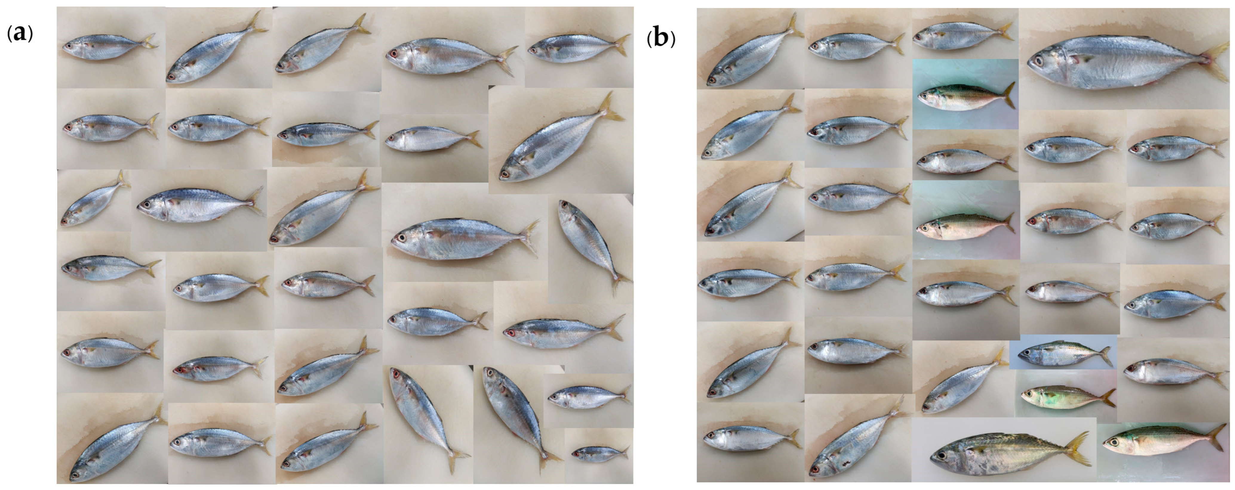
The images of both the
R. brachysoma and
R. kanagurta were captured by laying the fish horizontally on a 30 × 30 cm whiteboard placed on top of a table. Photographs were taken using the smartphone without any zooming function, utilizing default camera settings, without additional light sources or filters. Post-capture, all fish images were resized to cover from the tip of the snout to the end of the tail fin, as illustrated in
Figure 1.
In total, 517 images (267 of R. brachysoma and 250 of R. kanagurta) were randomly distributed into separate folders for training, validation, and testing purposes, organized into two classes: R. brachysoma and R. kanagurta. The training folder contained 183 R. brachysoma and 179 R. kanagurta images, while the validation set contained 56 R. brachysoma and 47 R. kanagurta images and the testing folder contained 28 R. brachysoma and 24 R. kanagurta images.
2.3. Image Processing
Due to the limited availability of 362 images for training, augmentation techniques were implemented to expand the dataset. This augmentation process assists in modelling by enhancing the capacity for better generalization and fortifying the model’s capability to handle novel, unseen data effectively throughout the training phase. The ImageDataGenerator class from Python’s Keras library was used for this purpose. The augmentation included rescaling (1/255), rotation up to 30 degrees, shifting width by 20%, shifting height by 20%, applying shear within 20%, zooming within 20%, enabling horizontal flipping, and using the ‘nearest’ fill mode. Finally, 11,584 images were acquired specifically for training purposes.
2.4. Deep Learning Algorithm Scheme
In this research, we utilized pre-trained deep learning models: ResNet-50, Xception, VGG16, VGG19, Inception V3, and MobileNetV3Small.
2.4.1. ResNet 50
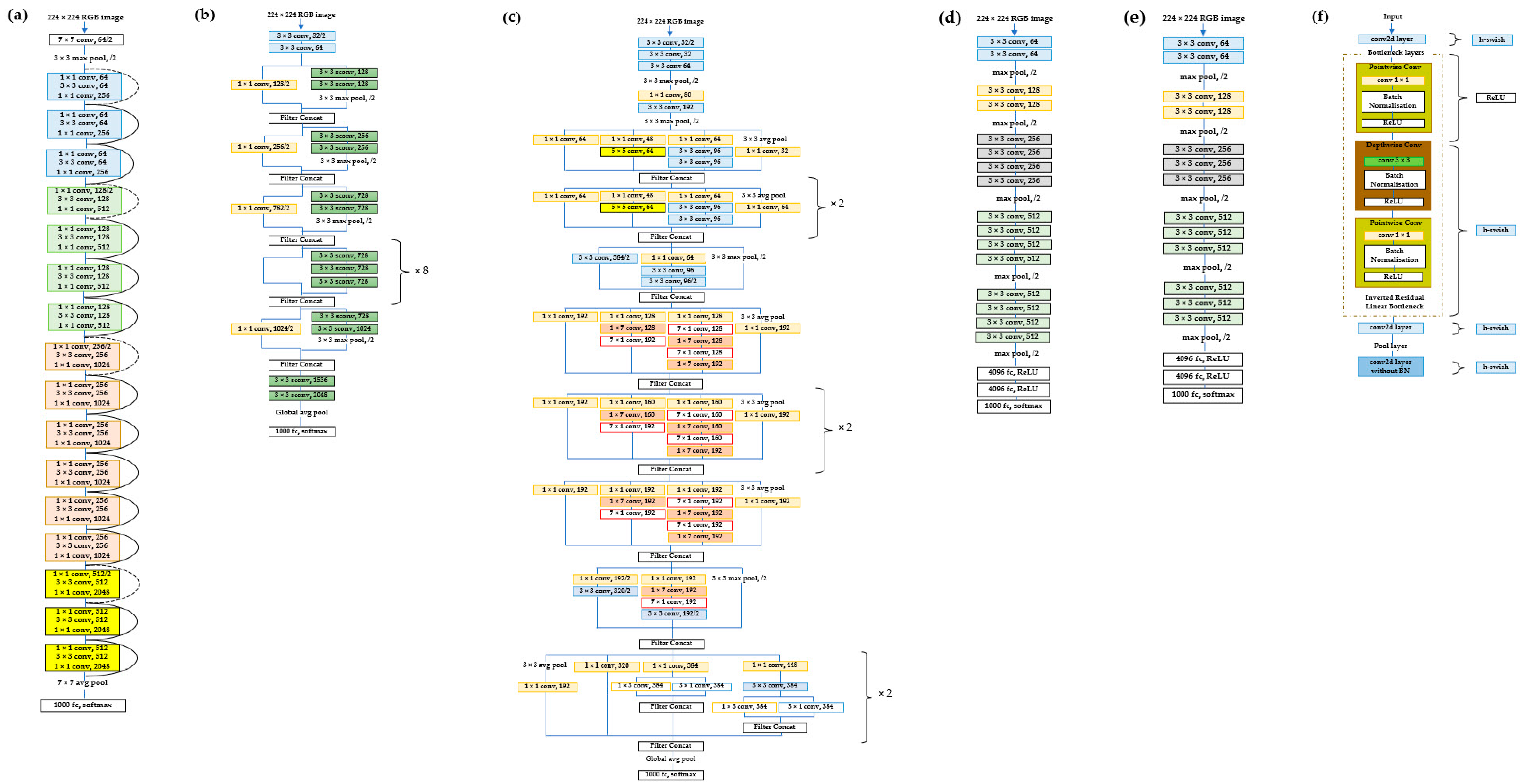
The ResNet-50 architecture consists of five stages, each featuring a convolutional block, an identity block, an average pooling layer, and a fully connected layer with 1000 neurons [
19]. In each convolution block, there were three convolution layers, and the same was applied to each identity block. The input size for ResNet-50 was 224 × 224 × 3. Following each convolutional layer, there was a batch normalization layer and a non-linear rectified linear unit (ReLU) function. Batch normalization layers standardized the activations of an input volume before passing it to the next layer, calculating the mean and standard deviation for each convolutional filter response across each mini-batch at each iteration to normalize the current layer activation. ResNet-50 comprised over 23 million trainable parameters. The original residual unit was adapted with a bottleneck design, as illustrated in
Figure 2a. Instead of the original 2-layered structure, a stack of three layers was used for each residual function F [
20].
2.4.2. Xception
This represents a CNN model and was developed by Google for object detection and image analysis, characterized as an advanced iteration of the Inception model. The architecture relies on layers of depth-wise separable convolution that outperform the Inception model. Notably, it introduces the idea that spatial correlations and cross-channel correlations in CNN feature maps can be entirely decoupled, presenting a more robust hypothesis compared to Inception.
The Xception architecture consists of 36 convolution layers, forming a foundation for efficient feature extraction. These layers are organized into 14 modules with linear residual connections enveloping them, except for the initial and final modules. It uses depth-wise separable convolution layers with linear residual connections in a linear stack, making it an easily definable and modifiable model. Its adaptability is facilitated by the use of a few lines of code and high-level libraries, such as Keras or TensorFlow [
21].
The inclusion of residual connections contributes to more rapid convergence, making it a superior performer in terms of both classification accuracy and processing speed. Each image undergoes entry flow, followed by middle flow, where the same process is iterated eight times, until finally proceeds through exit flow. Batch normalization follows all depth-wise separable convolution layers and convolution layers. With a depth multiplier set to one, ensuring no expansion of depth, Xception models have demonstrated excellent performance in convolutional neural networks, as illustrated in
Figure 2b, according to Chollet [
22].
2.4.3. InceptionV3
The Inception V3 model, depicted in
Figure 2c, is a pre-trained model by Google, having undergone training on more than 1000 classes and over 1.4 million images. This model serves as an image recognition tool for feature extraction, leveraging CNN. Subsequent classification is carried out through fully connected and softmax layers. Following this, a data sampler is applied to partition the data into training and testing sets [
22].
2.4.4. VGG19
VGG19 is a variation of the VGG model, comprising 19 layers. It consists of 16 convolution layers, three fully connected layers, five max-pooling layers, and a softmax layer. While conceptually similar to VGG16, the distinction lies in the number of layers, with nineteen denoting the count in this model. Trained on millions of images from the ImageNet database, VGG19 can categorize images into 1000 object categories, encompassing items such as pencils, keyboards, cars, and various animals [
21].
The input RGB image is presented in a fixed matrix dimension (224, 224, 3) and undergoes preprocessing by subtracting the RGB mean value from each pixel. Convolutional kernels of size (3, 3) with a one-pixel stride cover the entire image, preserving spatial resolution through the use of spatial padding. Max pooling of size (2, 2) is performed with a two-pixel stride, followed by ReLU activation to introduce non-linearity, enhancing the model’s classification performance and reducing computational time. This model has proven superior to previously used functions, such as tanh or sigmoid. It features three fully connected layers, with the first two having a size of 4096. Additionally, a layer with 1000 channels for the 1000 object categories of the ILSVRC classification is present, followed by a final softmax function, as illustrated in
Figure 2d, according to Humayun et al. [
21].
2.4.5. VGG16
VGG16, a CNN model designed for visual recognition, was introduced by Karen Simonyan and Andrew Zisserman from the Visual Geometry Group Laboratory at Oxford University in 2014. In the 2014 ImageNet Large Scale Visual Recognition Challenge, VGG16 secured first place in object detection within 200 classes and second place in classifying images labeled among 1000 categories. When applied to the ImageNet dataset containing 1000 classes with 14 million images, the model achieved an impressive 92.7% top-five test accuracy [
21].
The model accepts image inputs (dimensions 224, 224, 3) and comprises a total of sixteen layers. The initial two layers feature a 3 × 3 filter size and 64 channels with the same padding. Subsequently, a (2, 2) stride max-pool layer is followed by two 256-filter layers with a (3, 3) filter size, and another (2, 2) stride max-pool layer. Following this are two layers with a (3, 3) size and 256 filters, succeeded by two sets of three layers with 512 filters and a (3, 3) size convolution layer, along with a max-pool layer, all with the same padding. Then, the image undergoes processing through a stack of two convolution layers, applying 1-pixel padding after each convolution layer [
21].
Upon traversing all layers of VGG16, a (7, 7512) feature map is generated, which is subsequently flattened to obtain a (1, 25,088) feature vector. The model contains three fully connected layers; the first takes input from the last feature vector and produces a (1, 4096) vector, while the second yields the same output as the first and the third outputs 1000 channels corresponding to the 1000 classes. Then, the classification vector is normalized, passing from the third layer to the softmax layer [
23,
24]. The architecture is depicted in
Figure 2e.
2.4.6. MobileNetV3Small
MobileNetV1 [
25] was inspired from the traditional VGG architecture, while incorporating depth wise separable convolutions. Building upon this, MobileNetV2 [
26,
27] was introduced a year later, featuring a linear bottleneck and inverted residual. Subsequently, MobileNetV3 was developed with the assistance of neural architecture search (NAS) and NetAdapt networks for architecture optimization. This version drops expensive layers and adopts the h-swish non-linearity function instead of ReLU, aiming to enhance efficiency and maintain relative accuracy simultaneously, as of mid-2019.
MobileNetV3 is categorized into two models (MobileNetV3-Small and MobileNetV3-Large), with each tailored to low or high resource use cases, respectively, with their distinctive architectural complexity illustrated in
Figure 2f, according to Qian et al. [
25].
2.5. Model Creation
All the pre-trained models applied in this study were loaded and used as the base model. In addition, all model layers were frozen, preventing their weights from being adjusted during the training process. This allows the model to utilize the pre-trained weights from the ImageNet dataset. However, the final fully connected layer was removed, adding a global average pooling layer and two dense layers at the end, consisting of 1024 units followed by one unit, respectively. The activation function used in the final layer was Sigmoid, allowing the model to predict whether an image belonged to the specified class or not. The model was compiled by configuring the optimizer as Adam with a learning rate of 0.001. Binary cross-entropy served as the chosen loss function, while accuracy was applied as the evaluation metric.
Augmenting data can impact predictions both positively and negatively. On the positive side, it improves generalization and robustness by exposing the model to a wider range of data variations. However, this comes with drawbacks, such as increased computational cost and the risk of the model memorizing augmented samples, potentially worsening overfitting. To address this, we implemented an early stopping method to prevent overfitting. Additionally, the code utilizes the Model Checkpoint callback to save the best model weights during training, monitoring validation accuracy and storing only the optimal weights. The resulting file, ‘model_checkpoint.h5’, is stored in a Google Drive directory.
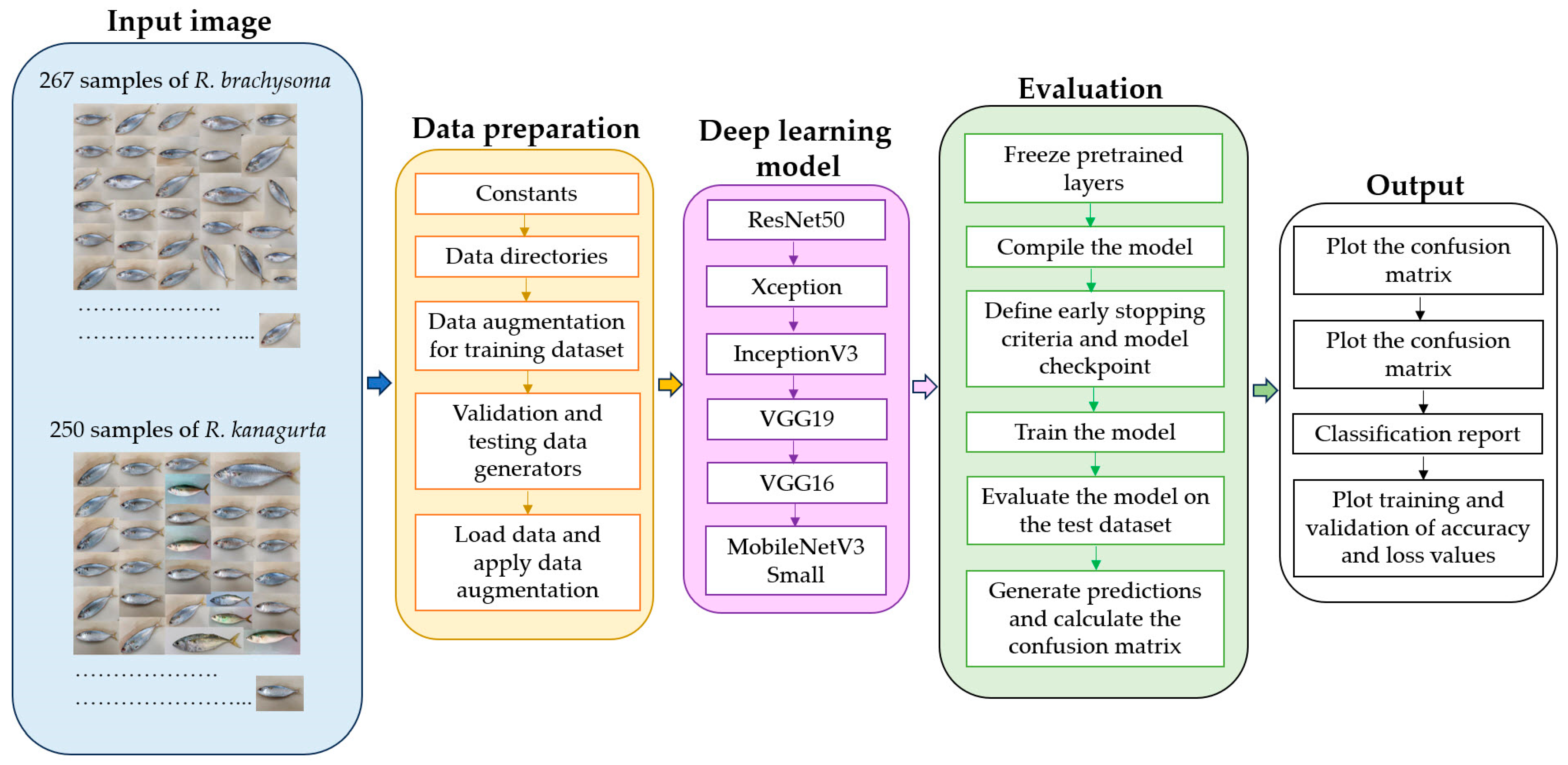
The flowchart of the deep learning algorithm constructed in this study is shown in
Figure 3 and
Table 2.
The best model from the previous outcomes was fine-tuned by increasing the number of epochs and further studying its performance.
2.6. Evaluation Indicator
Accuracy measures the proportion of correctly predicted samples out of the total number of samples in the dataset and was defined as (1):
where number of correct predictions is the total number of samples for which the model’s prediction matches the true target values in the dataset and total number of samples is the total number of samples in the dataset.
The loss function used was cross-entropy ad was defined as (2):
where
N is the number of samples in the dataset,
C is the number of classes,
yi,j is an indicator function that is 1 if the sample
i belongs to class
j and 0 otherwise, and
pi,j is the predicted probability that sample
i belongs to class
j.
Accuracy and loss values were computed for both the training and validation datasets across various pre-trained models. Subsequently, graphs were generated to visualize and display these metrics.
2.7. Classification Performance Metrics
Choosing appropriate indicators is a crucial factor in the scientific evaluation of the classification performance of deep learning models. Accuracy, precision, recall, and F1-score are commonly used as proven, effective, evaluation indicators. Accuracy refers to the percentage of correct results predicted in the total sample. Precision is the probability of an actual positive in all predicted positive samples. Recall is the probability of being predicted to be positive in actual positive samples, and the F1-score is the harmonic value of the precision rate and the recall rate. These indicators were calculated as shown in (3)–(6):
where, in Equations (3)–(5), TP is the number of positive classes predicted as positive classes, TN is the number of negative classes predicted as negative classes, FP represents the number of negative classes predicted as positive classes, and FN refers to the number of positive classes predicted as negative classes.
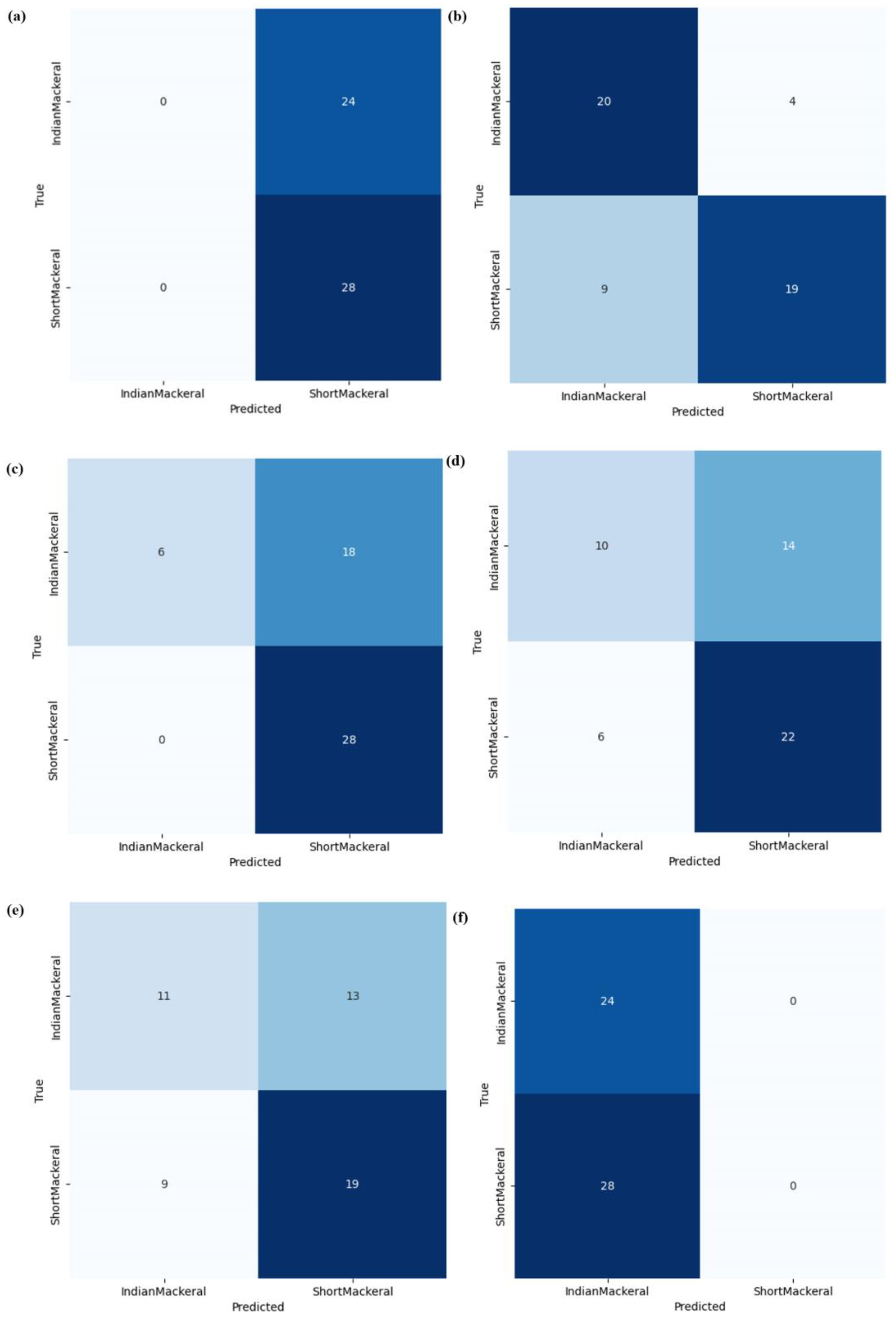
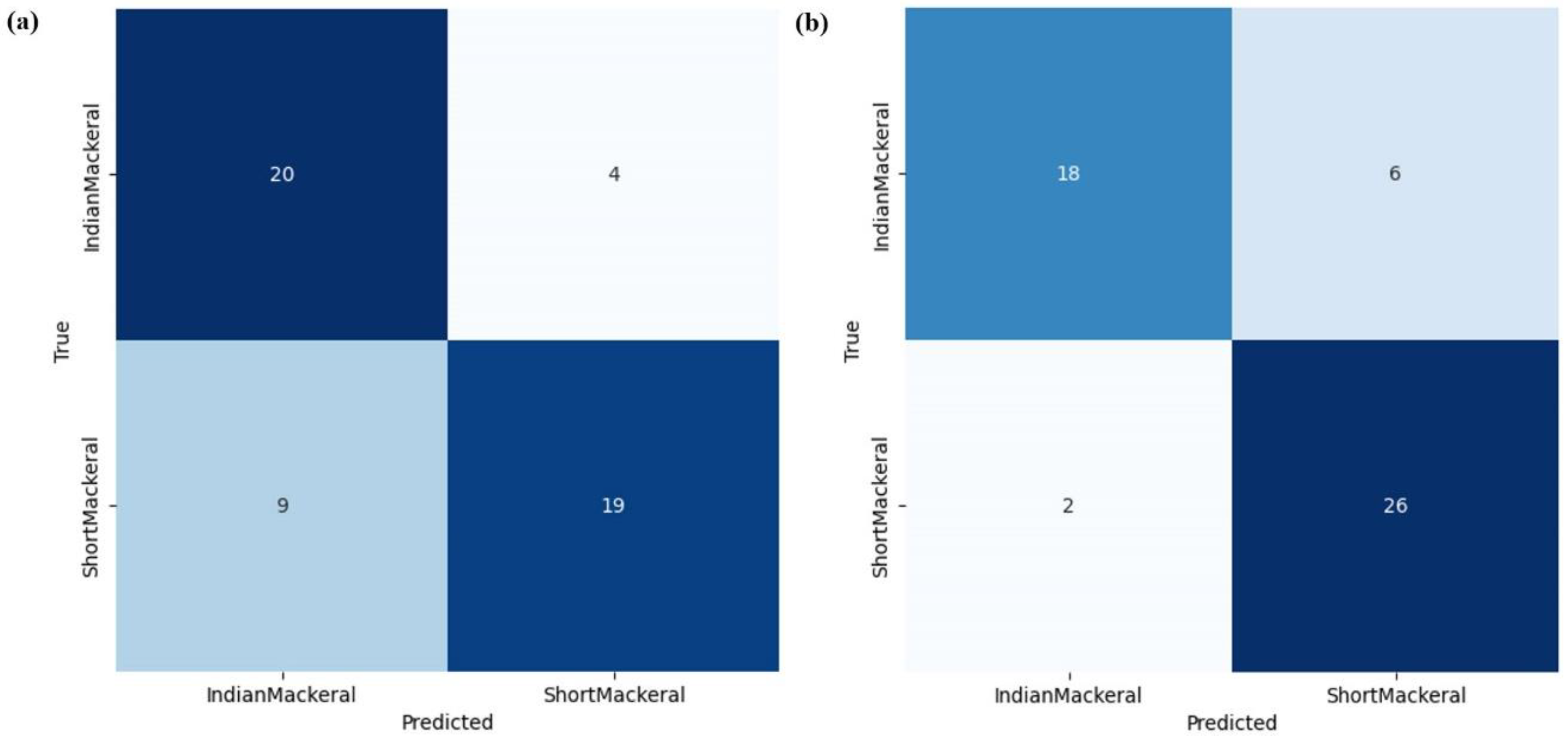
Confusion matrices were depicted using heat mapping to understand the model’s behavior in terms of correct and incorrect predictions.
3. Results and Discussion
3.1. Model Evaluation Based on Training, Validation, and Test Datasets
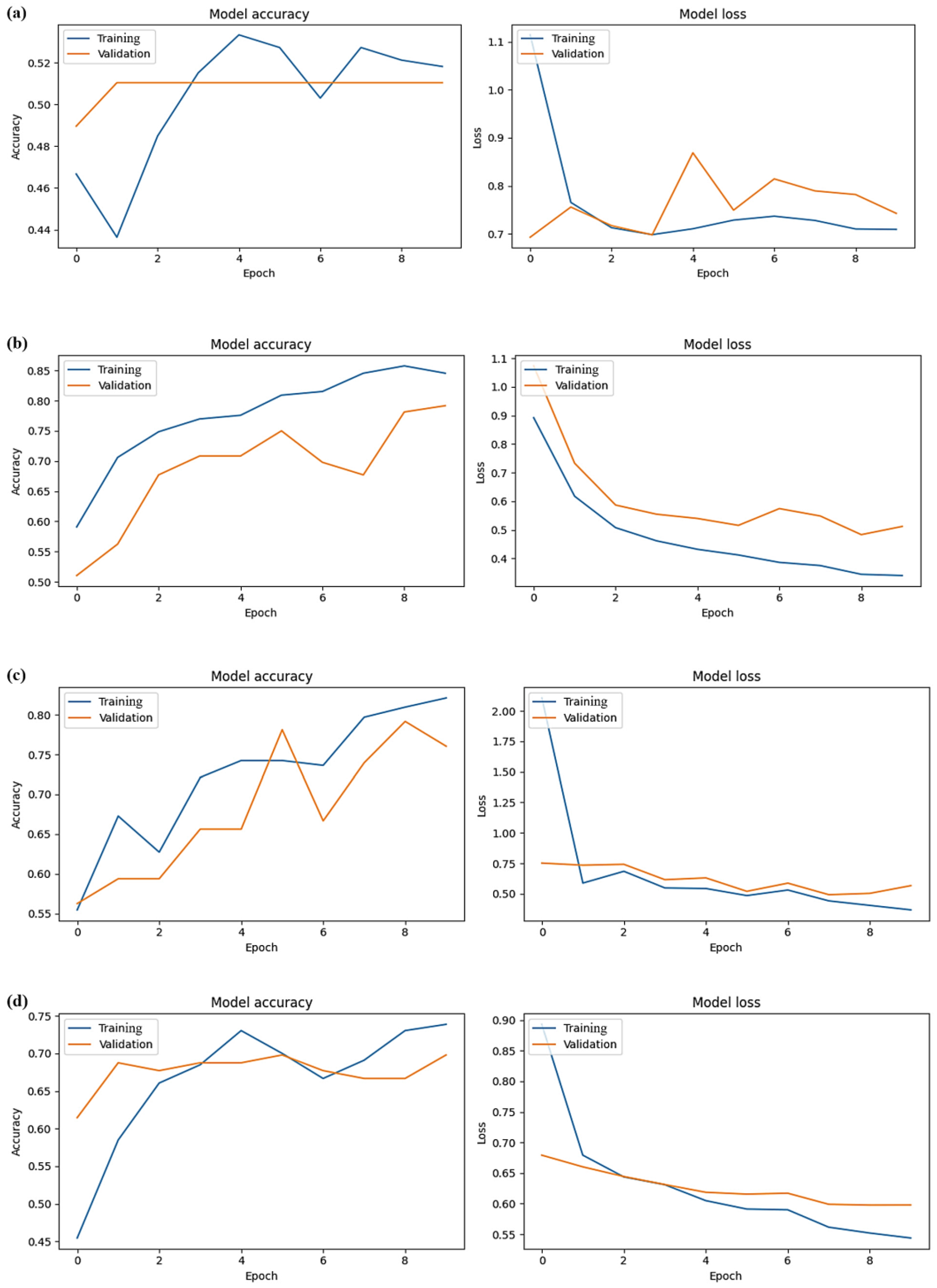
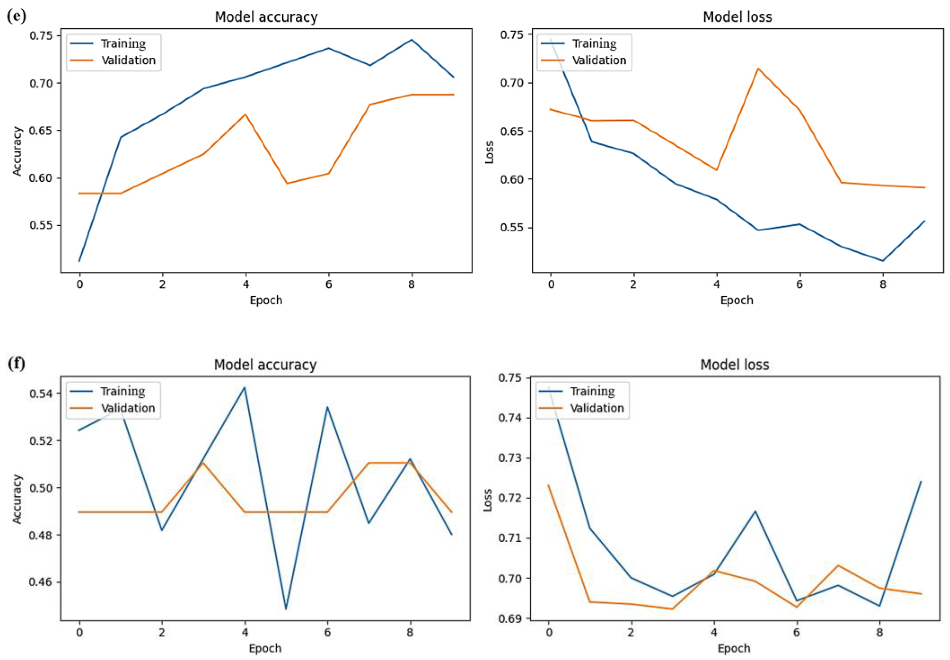
In the training and validation datasets, the Xception model demonstrated the best predictive performance, with the highest average accuracy levels of 0.849 and 0.754 for training and validation, respectively. In addition, the Xception model had the lowest average training loss of 0.505. However, in terms of validation, the Xception model was not quite as good as InceptionV3, with an average loss of 0.553 compared to 0.544 for InceptionV3. Overall, considering the comprehensive performance in the training and validation sets, the Xception model was the most efficient. Following it in descending order of performance were the InceptionV3, VGG19, VGG16, ResNet-50, and MobileNetV3Small models, as outlined in
Table 3 and illustrated in
Figure 4.
In the testing dataset, the Xception model had the highest values for average accuracy, recall, and F-1 score, with its precision score being slightly lower than for the InceptionV3 model. The average values for overall accuracy and for the precision, recall, and F-1 scores of the Xception model were at 0.757, 0.770, 0.748, and 0.750, respectively. The other models (InceptionV3, VGG19, VGG16, ResNet-50, and MobileNetV3Small) had overall accuracy values in descending order of 0.717, 0.620, 0.603, 0.560, and 0.513, respectively, as presented in
Table 4 and
Figure 5. Considering the cumulative results from training, validation, and testing, it was evident that the most suitable model for utilization was the Xception model, so it was further subjected to a fine-tuning process to enhance its performance in subsequent steps.
3.2. Fine-Tuning
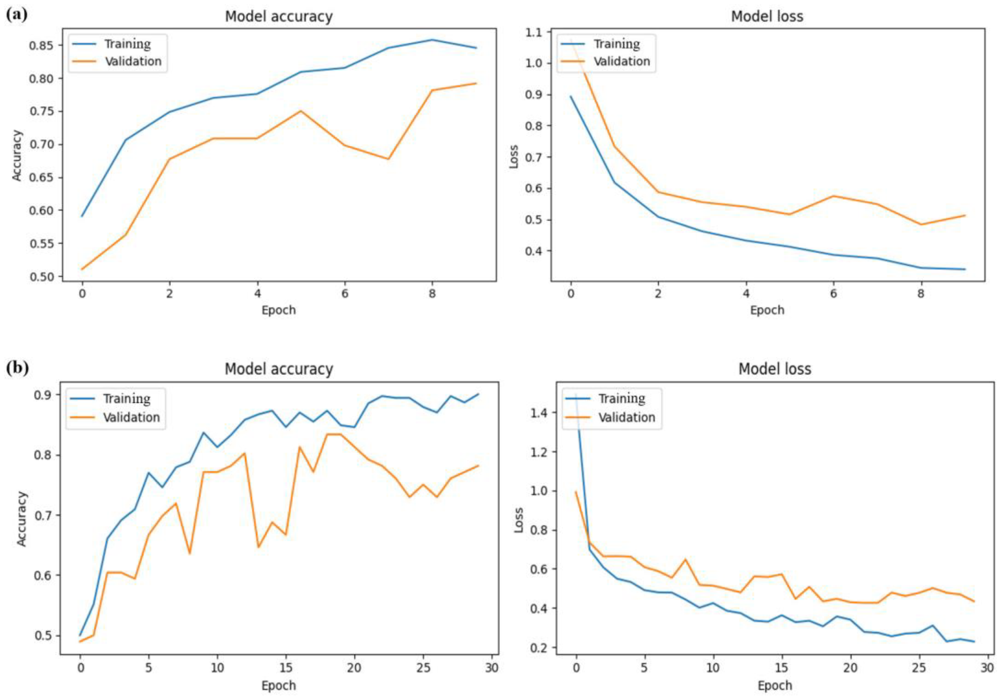
After fine-tuning the Xception model by increasing the number of epochs, the average accuracy increased substantially, reaching its peak at epoch 30 with a value of 0.896, while the average loss decreased substantially, hitting its lowest point at an average of 0.431 in the training set. At epoch 30, the model achieved its highest average accuracy of 0.799 and the lowest average loss of 0.427 in the validation set. However, upon extending the epochs to 35, for both the training and validation datasets, there was a decrease in average accuracy and increase in average loss, as outlined in
Table 5 and depicted in
Figure 6. Comparing epoch 30 to epoch 10, there was a clear increase in accuracy and a decrease in loss. However, extending beyond epoch 30 seemed to lead to a decline in both accuracy and loss.
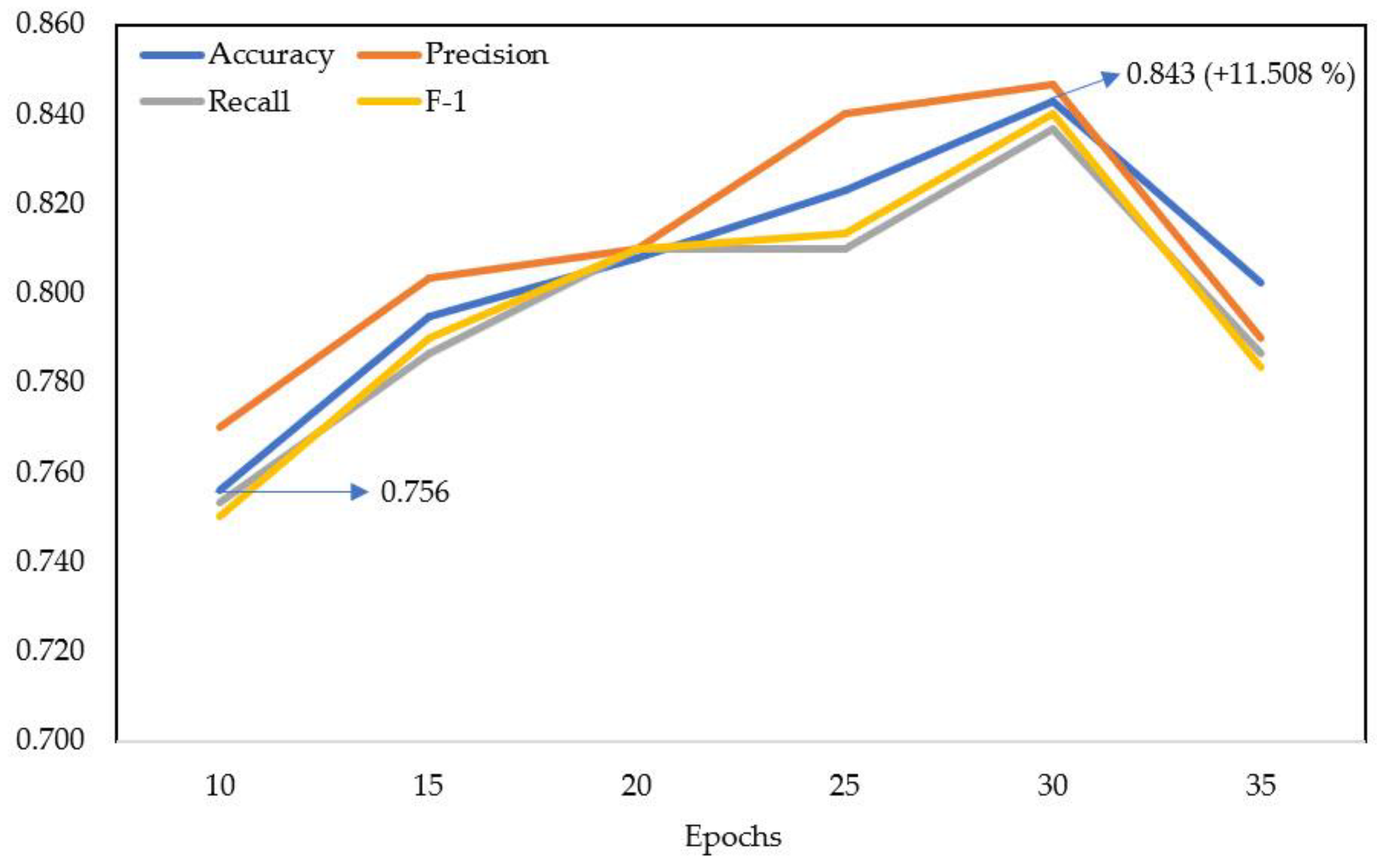
Based on testing over 10 epochs, the model had average values for accuracy, precision, recall, and F-1 score of 0.756, 0.770, 0.753, and 0.750, respectively. After enhancing the model performance by adding epochs every 5 epochs, the accuracy, precision, recall, and F-1 score consistently improved. With increments at 15, 20, 25, and 30 epochs, the values for average accuracy increased to 0.795, 0.808, 0.823, and 0.843, respectively; for precision to 0.803, 0.810, 0.840, and 0.847, respectively; for recall to 0.787, 0.810, 0.810, and 0.837, respectively; and for the F-1 score to 0.790, 0.810, 0.813 and 0.840, respectively.
However, similar to the training and validation datasets, extending epochs to 35 resulted in a decrease in the average performance metrics for the various model architectures. Therefore, utilizing 30 epochs provided the highest performance values for the model in terms of accuracy, precision, recall, and F-1 score in this study, as presented in
Table 6 and depicted in
Figure 7 and
Figure 8.
This study showed that images captured using a smartphone camera required pre-processing or augmentation to improve model performance. Smartphone-based image capture made the data collection more accessible and allowed for real-time species identification in the field, improving research efficiency and conservation efforts. The transfer learning models could be fine-tuned with smaller datasets specific to these diverse environments, improving their generalizability and real-world performance. Overall, applying transfer learning techniques to smartphone-captured images for the classification of R. brachysoma and R. kanagurta was very promising as a way of overcoming the limitations of previous research and advancing species identification in fisheries and in ecological studies.
The results of this study indicated that the Xception model had the highest performance of the test models, aligning with previous research [
12,
19,
28]. Compared to these findings, a similar study by Kurniawan et al. [
18] utilizing CNN had a higher testing accuracy of 0.947. However, that study used a camera setup, controlled lighting, and limited their classification to distinction between male
R. kanagurta and female
R. brachysoma fish. In contrast, the current study achieved a lower average testing accuracy of 0.843. The difference may have occurred since the current study did not prepare a controlled image-capturing environment, did not separate fish genders, and utilized mobile phones for image capture. This is the first known publication of using mobile phone for classification compared to other reported research that only identified different species that had external characteristic differences [
1,
29]. The use of a mobile phone is quite rare for identifying similar species with external characteristics quite similar to the fish species in the current study. We experimented with the MobileNetV3Small model, designed specifically for mobile use, to explore its feasibility. Its results from MobileNetV3Small were unsatisfactory, yielding an average testing accuracy of 0.513 across 10 epochs of processing. This requires further development moving forward. Contrasting the outcomes of this inquiry with the research carried out by Lu et al. [
17], our study focuses on the classification of species within aquatic environments using transfer learning. In comparison, Liu et al.’s study tackles the broader challenge of fine-grained visual categorization (FGVC), highlighting the significance of integrating detailed information from diverse layers of CNNs. Both studies highlight advancements in leveraging ML and DL for intricate visual recognition tasks.
The benefits of the current study were in aiding the conservation and management of species, which is especially critical given the vulnerability of R. brachysoma to overfishing. This approach should promote sustainable fisheries and help to combat illegal practices by facilitating traceability within the seafood trade. Leveraging smartphone cameras and transfer learning enhances accessibility and efficiency compared to traditional methods, making species identification more feasible. Additionally, it empowers scientists and fishermen to contribute data, enabling better monitoring of fish populations and supporting informed management decisions.
For enhanced accuracy in future study, it would be beneficial to gather more image data and to explore the potential of combined models while conducting further fine-tuning. For example, Akgül et al. [
13] applied the Xception model in a study of fish freshness detection, achieving successful results when combined with Yolo-v5 for anchovy (
Engraulis encrasicolus) and horse mackerel (
Trachurus trachurus). Additionally, comparing specific external fish body parts, such as color, fins, tail, body length, and width, might enhance classification performance.
The findings from this study should contribute toward the future development of a mobile phone application using images for fish species identification. Additionally, several recent studies have employed DL for fish morphology and behavior analysis. Petrellis [
30] investigated fish morphological features, including species like
Dicentrarchus labrax,
Diplodus puntazzo,
Merluccius merluccius, and
Sparus aurata, using image processing and DL techniques. Iqbal et al. [
11] utilized a CNN for classifying fish behavior. Wang et al. [
31] employed YOLOV5 and SiamRPN++ for real-time detection and tracking of fish abnormal behavior. The use of DL in classifying aquatic species presents an intriguing opportunity to investigate the relationship between morphological characteristics and behaviors in aquatic animals.

 ,
, 


