Article

Stock Discrimination of Gilthead Seabream (Sparus aurata Linnaeus, 1758) through the Examination of Otolith Morphology and Genetic Structure

by
George Geladakis
1,2,*,
Costas Batargias
1,
Stylianos Somarakis
3 and
George Koumoundouros
2
1
Biology Department, University of Patras, 26504 Rio, Patra, Greece
2
Biology Department, University of Crete, 70013 Heraklion, Crete, Greece
3
Institute of Marine Biological Resources and Inland Waters (IMBRIW), Hellenic Centre for Marine Research (HCMR), 71500 Heraklion, Crete, Greece
*
Author to whom correspondence should be addressed.
Fishes 2023, 8(6), 291; https://doi.org/10.3390/fishes8060291
Submission received: 25 April 2023 / Revised: 19 May 2023 / Accepted: 24 May 2023 / Published: 29 May 2023
(This article belongs to the Special Issue Morphometrics in Fisheries and Aquaculture)

Abstract

:
Reliable stock identification constitutes an integral component of effective fishery management. Current methods for the identification of putative stock units comprise the analysis of both phenotypic and genetic variability. The present study examined the spatial variation in otolith morphology (shape and asymmetry) and genetic composition of 395 wild-caught Gilthead seabream (Sparus aurata) specimens, collected from the Aegean and Ionian Seas (eastern Mediterranean) between 2014–2018. The degree of scale regeneration (SRD, % of regenerated scales) was used as an indicator to assess the potential presence of aquaculture escapees in the wild-caught samples. Otolith shape and asymmetry analyses showed a phenotypic discrimination between northwestern Aegean and Ionian Gilthead seabream populations. Genetic analyses of nine microsatellite markers revealed higher levels of genetic variation in the wild compared with samples obtained from aquaculture farms. Despite the absence of genetic structure among the wild-caught seabream populations, a low but statistically significant genetic differentiation was found between reared fish and fish collected in the field. The SRD was considered effective in detecting the presence of aquaculture escapees that may have escaped in either early or late rearing phases.
Key Contribution: The combined analysis of otolith and scale morphology proves adequate for distinguishing wild Gilthead seabream stocks: uncovering additional phenotypic variability resulting from the presence of aquaculture escapees in natural populations.

Graphical Abstract

1. Introduction

Gilthead seabream (Sparus aurata Linnaeus, 1758) is a highly valuable finfish for both fisheries and aquaculture industries in the Mediterranean Sea. Following FAO [1], global capture and aquaculture production of this species in 2020 was approximately 8646 tonnes and 282,073 tonnes, respectively. It is a coastal euryhaline marine fish with a natural distribution that extends along the eastern Atlantic coasts and the Mediterranean Sea, up to the Black Sea [2]. Previous studies have explored the natural genetic structuring of wild seabream populations across its entire distribution range using different genetic markers, including allozymes, mtDNA, microsatellites, and, recently, SNIPs (e.g., [3,4,5,6,7,8]). However, depending on the type and number of markers used, the existing literature on the genetic structuring of wild Gilthead seabreams has produced contradictory results with no evidence of simple isolation by distance among populations (e.g., [3,6,9,10]). Studies in both the Atlantic and Mediterranean Seas, at a variety of geographical scales, have indicated either an absence of genetic structure or a weak to strong population subdivision within and among different geographical areas (e.g., [7,8,11,12,13,14,15,16,17,18]). The long pelagic larval stage (up to 50 days at 17–18 °C in Gilthead seabreams [2,19]) is likely to contribute to migrant exchange among fish populations and seems to be one of the main reasons for the slight genetic differentiation and lack of geographic patterning among wild stocks in various fish species, including Gilthead seabreams (e.g., [11,12,20,21,22,23]). Additionally, accidental escapes of reared seabream, mainly due to technical or operational failures [24,25,26], or the release of gametes into the wild through spawning within sea-cages [27] may have impacted the genetic structure of local populations, potentially resulting in the introgression of foreign DNA into the wild gene pool. This hypothesis is further supported by the ability of reared escapees to survive in the natural environment for extended periods of time and to compete effectively for natural resources [28,29,30].
Except for genetic markers, a variety of methods and approaches have been proposed to discriminate wild fish stocks (namely self-reproducing fish groups that are available for exploitation in a given area, with the members of each group having similar life history characteristics [31]), including the analysis of phenotypic variability of different morphological traits of fish, such as body shape or otolith and scale morphology (e.g., [32,33,34,35,36,37]). Those traits are highly applicable in detecting differences in environmental conditions that fish experienced during their lifetime, particularly in the cases of marine species that breed in the open sea (e.g., Gilthead seabreams), where there are fewer barriers to dispersal and a small amount of gene flow between populations is sufficient to maintain the genetic homogeneity [12,20,22,38]. Previous studies have detected differences in body shape or in otolith and scale morphology between wild or between wild and reared Gilthead seabream populations of the western and eastern Mediterranean Sea [39,40], between fish of the wild and of a farmed origin in Greece [41,42,43] as well as between wild, reared, and farm-associated seabream populations across the Adriatic Sea [16,44,45,46].
Otoliths are calcified structures found in the inner ears of teleosts and involved in hearing and balance systems [47]. They consist of a calcium carbonate material that is deposited continuously on an organic matrix throughout the fish’s lifetime. Unlike scales and bones, otoliths are metabolically inert (i.e., once deposited, otolith material is unlikely to be resorbed or altered) and contain reliable fingerprints that provide information for the entire life cycle of the fish [48,49,50]. The otolith shape results from the combined expression of its genotype and the conditions of the growing environment [51,52,53,54,55,56,57,58]. However, it also depends on the fish’s developmental stage, age, body size, sex, or sexual maturity status (e.g., [50,51,59,60,61,62,63,64]). At the individual level, bilateral differentiation in biomineralization processes induce morphological differences between the left and right pair of otoliths. At the population level, otolith fluctuating asymmetry (FA) refers to the random deviations from perfect bilateral symmetry induced by differences between the left and right body sides [65]. Due to the high functional value of the otolith structures in fish balance and hearing [66,67], otolith FA is considered a sensitive indicator for examining the effects of environmental stress and/or environmental heterogeneity on the health status of wild fish populations (e.g., [68,69,70,71,72]).
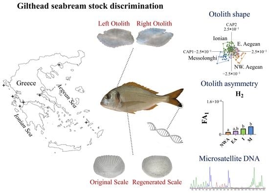
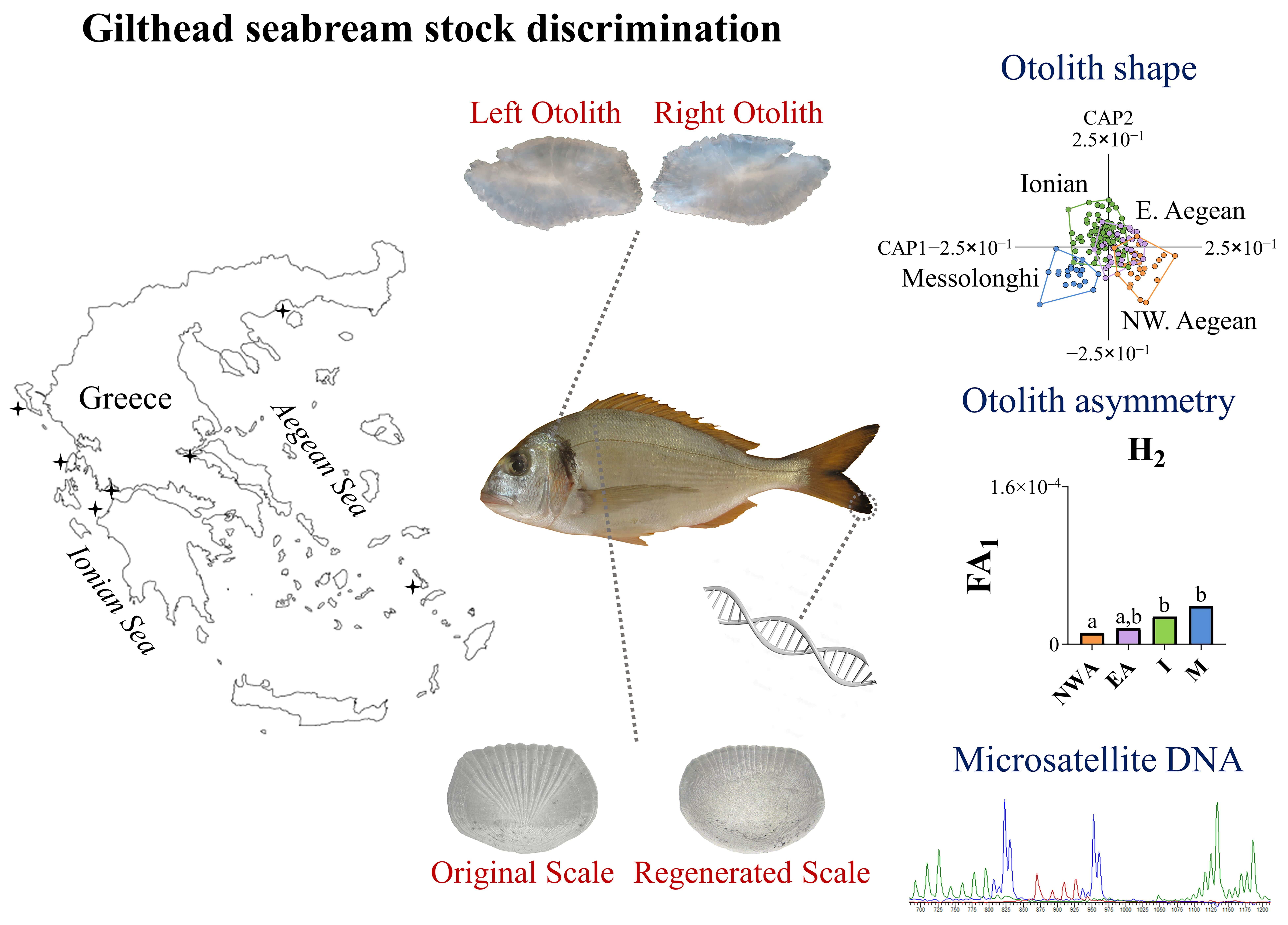
In the present study, we investigated the genetic population structure and spatial variation in the shape and asymmetry of otoliths in wild-caught Gilthead seabreams sourced from the Aegean and Ionian Seas (eastern Mediterranean). To control for the potential presence of aquaculture escapees among wild-caught individuals, we used the degree of scale regeneration (SRD, % of regenerated scales), which has been shown to be significantly higher in reared fish [40,41,42,73,74], as an indicator to exclude potential aquaculture escapees (as previously demonstrated by [41]) in the comparisons of otolith morphology (shape and asymmetry) and genetic composition between wild-caught fish of different geographical origins.

2. Materials and Methods

2.1. Sample Origin and Scale Examination

A total of 395 Gilthead seabreams were used for this study (Table S1). All fish were caught in the field from the North (Kavala), West (Maliakos Gulf), and East (Kalymnos) Aegean Sea; from different areas of the Ionian Sea (Patraikos Gulf, Central Ionian Sea, Corfu); as well as from the Messolonghi lagoon (Western Greek coast) between 2014–2018 (Tables S1 and S2, Figure 1). In the Ionian Sea, fish were collected with an experimental bottom trawl onboard the R/V PHILIA. In the Aegean Sea, the samples were obtained onboard small scale fishing vessels (netters), and in the Messolonghi lagoon, samples were obtained from the seasonal (autumnal) trap fishery, which take place during the mass seaward migrations of the species from the lagoon to the open sea, prior to the spawning season [75]. Depending on geographical origin, the fish samples were assigned into four groups: northwestern Aegean (NWA), East Aegean (EA), Ionian (I), and Messolonghi (M). Given that coastal lagoons exhibit large fluctuations in abiotic parameters [76], the study also aimed to investigate the effect of the specific environmental conditions of the Messolonghi lagoon during the period when it serves as a nursery ground for the fish [77] on the otolith morphology of wild Gilthead seabreams.
In the laboratory, fish were measured for standard length (SL, tip of snout to base of the central caudal lepidotrichia) and the largest pair of otoliths (sagittae) were extracted from each specimen. All otoliths were cleaned in 75% ethanol and individually photographed against a dark background with reflected light using a digital camera (Lumenera INFINITY1-5C, Teledyne Lumenera, Ottawa, Ontario, Canada) attached to a stereoscopic microscope (Olympus SZ61, Olympus Europa SE and Co., KG, Hamburg, Germany). A sample of 20 scales was then randomly removed from the left side of each fish, within the region between the anterior dorsal fin and the lateral line. Scales were photographed and examined for the presence or absence of a regenerated nucleus. The degree of scale regeneration (% regenerated scales) (SRD) was then calculated for each specimen (e.g., [74,78]). Within each geographic group, in order to assess potential temporal changes in SRD, Kruskal–Wallis and Mann–Whitney U tests were performed between the SRD of fish collected in different years.
In the present study, to minimize any effects of the possible presence of aquaculture escapees in the examined samples, the SRD was used to assign wild-caught fish into one of three predetermined groups: (a) fish with SRD lower than 30% (L30), (b) fish with SRD between 31–60% (31–60), and (c) fish with SRD higher than 60% (M60). Following Geladakis et al. [41,74], wild-caught seabreams with SRD higher than 30% (50% of fish specimens, Geladakis et al. [41]) had an increased possibility of including fish that escaped from net pens at various phases of the rearing process.
Two additional Gilthead seabream samples from two commercial cage farms, one from the northwestern Aegean (NWAR, n = 30) and another from the Ionian Sea (IR, n = 28), were also included in this study to serve as reference points for the genetic analysis of wild-caught specimens.

2.2. Otolith Shape Analysis

To ensure consistent orientation between otoliths from both sides of the body, the images of right otoliths were horizontally flipped. Using conventional image analysis techniques, all captured images were transformed to binary (ImageJ software version 1.3 k, U. S. National Institutes of Health, Bethesda, MD, USA [79]) and further analyzed by using the ShapeR package [80], an open software in R (version 4.0.3, R Foundation for Statistical Computing, Vienna, Austria [81]). Otolith outlines were automatically extracted from the images and each otolith shape was then represented by a two-dimensional coordinate matrix (x, y) for further analysis. Primarily, four univariate morphological descriptors were calculated for each otolith outline: surface area (OS, mm2), perimeter (OP, mm), maximum length (OL, mm), and maximum depth (OD, mm). Based on the criterion of 98.5% accuracy for otolith reconstruction, a normalized elliptic Fourier approach was used to create a total of 12 harmonics, each one composed of four coefficients [80]. Otolith shape data were standardized and aligned with respect to size by omitting from the analysis the first three harmonic coefficients (resulting in 45 coefficients out of the initial 48). In order to adjust otolith shape with respect to allometric relationships with fish standard length (SL), those Fourier coefficients exhibiting a significant interaction (p < 0.05) between groups and fish SL were also excluded from the analysis [80].
Elliptic Fourier data of wild-caught individuals were first analyzed for differences between fish of different origin (NW. Aegean, E. Aegean, Ionian, Messolonghi) and SRD levels (L30, 31–60, M60) using multivariate nonparametric analysis of variance (PERMANOVA [82]). PRIMER-E software (version 6, Plymouth Routines in Multivariate Ecological Research, Plymouth, UK [83]) with the PERMANOVA add-on was used to transform the elliptic Fourier coefficients to a Euclidean distance matrix. PERMANOVA was performed on the partitioned sums of squared Euclidean distances to generate the distribution of the pseudo-F statistic using unrestricted permutation of raw data (9999 permutations [84]). Respective p-values were also estimated for the statistical significance of the tests. To evaluate the arrangement and differentiation among groups in multivariate space, the Euclidean distance matrix was subjected to canonical analysis of principal coordinates (CAP [85]). The determination of the number of PCO axes (m) was guided by the calculation of the minimum misclassification error based on the “leave-one-out” approach. An a priori hypothesis regarding distinct sample groups was tested using CAP by obtaining a p-value through 9999 permutations [83].

2.3. Otolith Bilateral Asymmetry

Eight traits were used to assess bilateral asymmetry: four univariate morphometric descriptors (OL, OD, OS, OP) and four high-amplitude harmonics (H2–H5) (i.e., low-order harmonics, which describe the main outline characteristics of otolith contour [86]). Amplitudes were derived from the elliptic Fourier coefficients of each harmonic descriptor without adjustment for fish standard length (SL) [41]. The following equation, as described by Tort [86], was used to calculate the amplitude of harmonic n for each otolith:
a m p n = 1 2 a n 2 + b n 2 + c n 2 + d n 2
Primarily, all traits were assessed for the type of bilateral asymmetry, namely fluctuating asymmetry, directional asymmetry, or antisymmetry [69,87]. Fluctuating asymmetry (FA) is considered ideal when the distribution of right minus left measurements (R-L) has a zero mean and follows a normal variation. On the other hand, directional asymmetry (DA) is characterized by a significantly skewed R-L distribution while antisymmetry displays either bimodal or platykurtic distribution characteristics [88]. According to Palmer and Strobeck [89], conventional skew and kurtosis statistics are considered powerful tests to examine departures from normality as they provide additional insights into the variation between sides. One-sample t-tests were performed to determine whether the R-L distribution of the otolith traits displayed skewness (g1) and kurtosis (g2) equal to zero [90]. To examine the potential correlation between asymmetry and fish size, a straightforward regression analysis was conducted by assessing the natural logarithm of the absolute bilateral difference (ln|R-L|) in relation to size (SL) for each trait [69,87].
To quantify the degree of otolith asymmetry, the variance of the bilateral difference (FA1 = var(R-L)) was computed for each trait and fish group [91]. Bonferroni-corrected F-tests were applied to test for significant differences in FA1 among the different groups [88].

2.4. Microsatellite DNA Analysis

A small piece of caudal fin tissue was cut from each fish and stored in 99.9% ethanol. Total genomic DNA was extracted by Chelex-100 (5%) following the DNA isolation protocol as described in [92]. Fish DNA was genotyped with the following nine microsatellite markers: D67, SAGT1, VBC003, Bd10, ELD10, BMAP54, SGAT32, VBC160, SAGT41 [93,94,95,96]. For the simultaneous amplification of the nine microsatellite loci, multiplex PCRs were run in 13.3 μL total volume reactions containing 4.5 μL of KAPA2G Fast Multiplex PCR mix (Kapa Biosystems, Potters Bar, United Kingdom), ~50 ng template DNA, and Primers with a final concentration of 0.1–0.5 μΜ. PCR cycling conditions consisted of an initial 95 °C denaturation step for 3 min, followed by 35 cycles of 30 s at 94 °C., 30 s at 56 °C, and 30 s at 72 °C, with a final elongation step at 72 °C for 45 min. The ABI3500 automated sequencer (Applied Biosystems, Carlsbad, CA, USA) was used to separate microsatellite fragments while to determine the size of alleles, the produced electropherograms were analyzed using STRand software (version 2.4.110, Veterinary Genetics Laboratory, Davis, CA, USA [97]).
The possible presence of null alleles and genotyping errors in the dataset was tested using MICROCHECKER software (version 2.2.3, University of Hull, Hull, UK [98]). Significant deviation from Hardy–Weinberg equilibrium (HWE) for each locus and fish group were tested using GENEPOP (version 4.7.5, University of Montpellier, Montpellier, France [99]). Microsatellite toolkit (version 3.1.1, Animal Genomics Lab, University College Dublin, Ireland [100]) was used to calculate observed (Ho) and expected (He) heterozygosity as well as the mean number of alleles across all loci (A). The mean effective number of alleles across loci (Ae) was calculated using POPGENE (version 1.32, University of Alberta, Alberta, Canada [101]). FSTAT (version 2.9.4, UNIL, Lausanne, Switzerland [102]) was used to calculate inbreeding coefficient (FIS) and allelic richness (Ar) and to perform an exact test for linkage disequilibrium between loci. Global and pairwise FST values were calculated in Arlequin (version 3.5.2.2, University of Bern, Bern, Switzerland, [103]) using 10,000 permutations to test for statistical significance. All multiple pairwise tests were adjusted using Bonferroni corrections [104].
To further analyze the genetic relationships among wild-caught fish groups, a Bayesian clustering analysis was performed using STRUCTURE software (version 2.3.4, Stanford University, Stanford, CA, USA [105]). The model-based clustering method was run assuming a number of K populations ranging from one to ten (maximum number of groups examined). For each K, burn-in period was set to 100,000 interactions followed by 1,000,000 MCMC repetitions, using an admixture model without a priori structuring information. STRUCTURE results were analyzed with the CLUMPAK online software (Tel Aviv University, Tel Aviv, Israel [106]) to detect the best K value using the Evano method [107] and DISTRUCT feature [108] to visualize the optimal number of clusters. Finally, two same Structure analyses were also conducted to analyze the genetic relationships between reared and wild-caught fish of the same origin, one for the northwestern Aegean Sea and another for the Ionian Sea.

3. Results

3.1. Degree of Scale Regeneration (SRD)

Significant differences were found in the average degree of scale regeneration (SRD) among samples collected in different years within each geographic group of fish (p < 0.05, Kruskal–Wallis and Mann–Whitney U tests) (Figure 2A–D). More precisely, concerning the northwestern Aegean Sea, significant differences in the average SRD levels were observed between samples collected in 2015 and 2017 (Figure 2A). Regarding the Ionian Sea, significant deviations in SRD levels were detected among samples collected in 2014 and those from 2015 and 2018, as well as between samples taken in 2015 and 2017 and between 2017 and 2018 (Figure 2C). The average (±SD) SRD varied among groups from 34.6 ± 22% (East Aegean) to 52.7 ± 33.0% (northwestern Aegean) (Table 1). The proportion of wild-caught fish in the predetermined SRD groups also varied depending on their origin, ranging from 36.8% (northwestern Aegean) to 53.8% (East Aegean) for the group L30, 22.4% (northwetsern Aegean) to 34.6% (Ionian) for the group 31–60, and 13.8% (East Aegean) to 40.8% (northwestern Aegean) for the group M60 (Table 1, Figure S1).

3.2. Otolith Shape

For both left and right sides of the body, PERMANOVA showed that fish origin had a significant effect on otolith shape (Table 2). The effect of SRD level was not statistically significant for both the left and right otoliths (Table 2). Finally, the interaction between fish origin and SRD was significant for the right but not the left otolith (Table 2).
For the right otolith, following the PERMANOVA model of interaction between fish origin and SRD, pairwise comparisons showed that fish with low and moderate levels of scale regeneration (L30 SRD and 31–60 SRD) from the northwestern Aegean Sea and the Messolonghi lagoon had significantly different otolith shapes compared to the other geographic groups (Table 3). However, there were no significant differences in otolith shape between fish from the East Aegean and the Ionian Sea (Table 3). In individuals with SRD levels > 60% (M60 SRD), the only significant difference in otolith shape was observed between fish from the Ionian Sea and those from the northwestern Aegean Sea and Messolonghi lagoon (Table 3). Finally, when we tested for differences in otolith shape between fish with different SRD levels within each geographic location, significant differences were found between fish with M60 SRD and those with L30 or 31–60 SRD in the northwestern Aegean and Ionian Seas (Table S3).
The canonical analysis of principal coordinates (CAP) showed that otolith shape differentiation among fish with a different geographical origin increased with the increased level of SRD for both body sides (31–60 and M60; Figure 3). All CAP analyses presented highly significant permutation statistics (for details see Appendix A, Tables S4 and S5).
In the case of the left side of the body, for the fish with an L30 SRD, the first canonical axis (squared canonical correlation of CAP1 δ12 = 0.776) separated the geographic groups of the Aegean (NW. Aegean and E. Aegean groups) from those of the Ionian Sea (Ionian and Messolonghi lagoon groups) while the second canonical axis (CAP2) was not related to any meaningful geographical differentiation (Figure 3). In fish with a 31–60 SRD, CAP1 (squared canonical correlation δ12 = 0.672) separated the fish group of the NW. Aegean Sea from the other groups, whereas CAP2 was also not related to any meaningful geographical differentiation. In fish with an M60 SRD, CAP1 (squared canonical correlation δ12 = 0.657) separated the group of the Messolonghi lagoon from the other geographic groups, and CAP2 separated the groups of the Aegean from those of the Ionian Sea (Figure 3).
In the case of the right side of the body, for the fish with an L30 SRD, the first (squared canonical correlation of CAP1 δ12 = 0.454) and second (CAP2) canonical axis did not reveal any meaningful geographical differentiation between groups. For the fish with a 31–60 SRD, CAP1 (squared canonical correlation of CAP1 δ12 = 0.746) discriminated the fish group of the northwestern Aegean from the groups of the Ionian and E. Aegean Sea (Figure 3) while CAP2 was related to the differentiation between the group of Messolonghi and the other geographic groups. Finally, in fish with an M60 SRD, CAP1 (squared canonical correlation δ12 = 0.687) separated the group of Mesolonghi lagoon from the groups of the Ionian and northwestern Aegean Sea (Figure 3), whereas CAP2 separated the fish of the northwestern Aegean from the fish of the Ionian Sea (Figure 3).

3.3. Otolith Bilateral Asymmetry

The asymmetry of the otolith perimeter and harmonic 3 showed a significant correlation with the fish SL (p < 0.01, not shown). Thus, a ratio transformation was applied prior to the calculation of the FA1 index for these two otolith traits, with (R-L) values divided by (R + L)/2 [91]. Antisymmetry was absent, with all kurtosis estimates (g2) being either non-statistically different from zero or significantly positive (Table 4). Interestingly, directional asymmetry was detected for three of the otolith size descriptors, OS, OP, and OL (skew significantly negative, R < L), and the shape descriptors H2 and H5 (skew significantly positive, R > L) (Table 4). However, fluctuating asymmetry indices based on signed R-L values (e.g., FA1) are not biased by skewed distributions [88].
Otolith asymmetry analysis within each geographic location revealed that the degree of scale regeneration (SRD) had a significant effect on otolith shape fluctuating asymmetry (FA) in three out of the four geographic groups (northwestern Aegean, Ionian, and Messolonghi). Specifically, fish of M60 SRD exhibited significantly higher FA1 in the shape descriptors H2 and/or H4 when compared to the other SRD categories (L30 and 31–60 SRD; Figure S2).
The geographic origin of the fish had a significant effect on the otolith FA. In individuals with an L30 SRD, depending on the descriptor examined, the fish from Messolonghi lagoon displayed significantly higher (i.e., H2) or lower (i.e., H4) otolith asymmetry compared to other groups (i.e., northwestern Aegean and Ionian groups; Figure 4). Additionally, the shape descriptor H2 exhibited significantly higher fluctuating asymmetry in fish from the Ionian Sea compared to the northwestern Aegean Sea (Figure 4). In individuals with a 31–60 SRD, for the descriptors OL and H3, FA1 was significantly higher in the northwestern Aegean Sea than in the Messolonghi lagoon (Figure 4). Furthermore, in fish with an M60 SRD, the shape descriptor H2 exhibited significantly higher FA in the Ionian Sea compared to the other geographic groups (Figure 4).

3.4. Genetic Diversity

A total of 286 wild-caught fish and 55 reared fish were successfully genotyped at 9 microsatellite loci with no missing genotype within the dataset. Micro-Checker did not detect null alleles or genotypic errors using 95% confidence intervals. Between all pairs of loci, there was no consistent evidence of linkage disequilibrium following a strict Bonferroni correction for multiple tests. All fish groups appeared to be in Hardy–Weinberg equilibrium (p > 0.05, Fisher’s exact test).
Genetic diversity varied among wild-caught fish groups of different geographical origins and degrees of scale regeneration (SRD), ranging from 8.67 to 16.11 in the number of alleles (A), 6.70 to 9.42 in the effective number of alleles per locus (Ae), 8.54 to 9.08 in allelic richness (Ar), as well as 0.85 to 0.92 and 0.85 to 0.88 for the observed (Ho) and expected (He) heterozygosity, respectively (Table S6). Summarizing the results in respect to SRD levels (Table 5), it was obvious that there was a clear negative correlation between the SRD levels and the magnitude of the genetic parameters A, Ae, and Ar of the different groups. Among wild-caught groups, the fish with the lower SRD (L30) exhibited the highest values of the genetic parameters, whereas the fish with the higher SRD (M60) exhibited the lowest values.
Reared Gilthead seabreams exhibited lower genetic diversity in A, Ae, Ar, Ho, and He compared to wild-caught counterparts for both regions (northwestern Aegean and Ionian Seas), whereas the reared fish from the Ionian Sea showed the lowest values in all the examined genetic parameters compared to the northwestern Aegean reared fish (Table 5 and Table S6).

3.5. Genetic Structure and Individual Assignment

Considering only the wild-caught groups, the global FST exhibited a null value (−0.00045, p > 0.05), indicating a lack of genetic differentiation among geographic groups and SRD levels. This result was supported by the respective pairwise FST estimations, analyzed either as an origin within SRD groups (Table S7) or vice versa (Table S8).
Taking into account wild-caught (with different SRD levels) and reared groups, global FST values showed 0.008 (p < 0.001) and 0.014 (p < 0.001) for the northwestern Aegean and Ionian Sea, respectively, revealing slight indication of genetic differentiation between wild-caught and reared fish. Pairwise FST analysis revealed statistically significant differences only between reared and wild-caught fish groups (L30, 31–60, M60) for both the northwestern Aegean and Ionian Seas. (p < 0.01, Table 6). It is worth noting that the FST values of the Ionian reared group was almost double that of the northwestern Aegean in all pairwise comparisons.
Clustering analysis for all the wild-caught fish suggested the presence of 6 clusters (K = 6) as determined by the ΔΚ procedure (Figure 5A). Fish groups were assigned to the six clusters with equal distribution and proportion of individual membership in each cluster (16.7%).
The results of the clustering analysis for the reared and wild-caught fish from both the northwestern Aegean and Ionian Seas revealed that the optimal number of clusters (K) was three (Figure 5B,C). The wild-caught fish groups of L30, 31–60, and M60 SRD were assigned to two separate clusters, with a total proportion of membership to these clusters ranging from 82.6% to 90.2% for both seas. The third cluster was associated with a reared origin, with an average individual membership proportion of 57% and 82.1%, for the reared fish from the northwestern Aegean and Ionian Sea, respectively (min: 5.1%, max: 97.6%). Additionally, 16 out of 64 northwestern Aegean (7 from L30, 2 from 31–60 and 7 from M60) and 27 out of 159 Ionian (13 from L30, 8 from 31–60 and 6 from M60) wild-caught individuals were not effectively assigned to clusters associated with wild origin, resulting in total individual membership proportions to these clusters of less than 82%.

4. Discussion

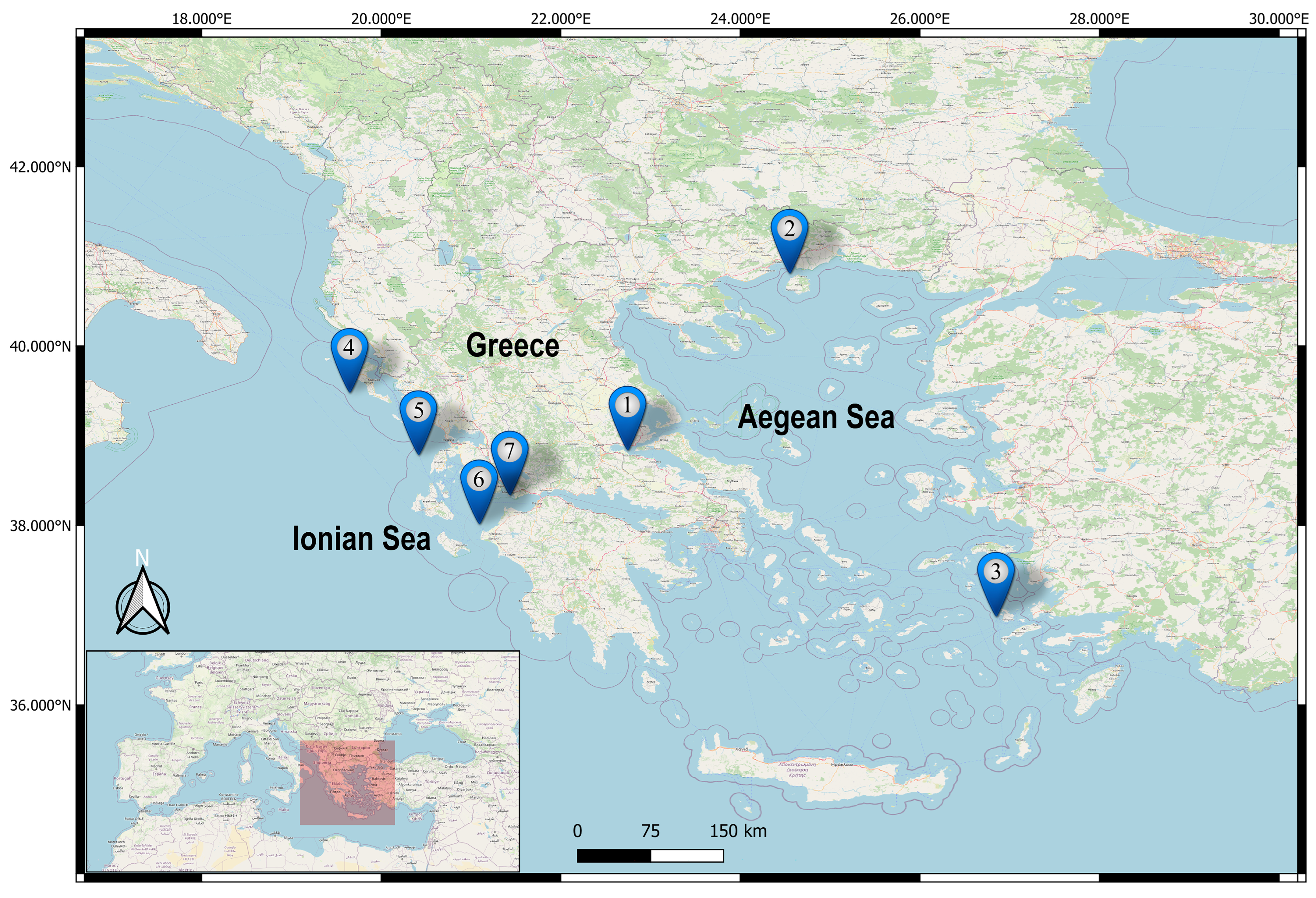
In the present study, otolith shape and asymmetry analyses of wild-caught fish with a low possibility of being aquaculture escapees (L30 SRD group) revealed a phenotypic discrimination between northwestern Aegean and Ionian Gilthead seabream populations. However, a genetic analysis indicated an absence of genetic differentiation among the studied geographic fish groups. The otolith shape is a popular tool used for the discrimination among fish populations (e.g., [53,109,110]) with significant value as an indicator of stock identity (e.g., [47,58]). The otolith shape has been shown to be affected by both biotic and abiotic environmental drivers during fish development, including water temperature [60,111,112,113], habitat depth [114], type of substrate [115], acidification levels [116], food quantity [117], and food composition [55,112]. Geladakis et al. [35] suggested that observed phenotypic variability among wild fish stocks of the European sardine (Sardina pilchardus Walbaum, 1792) could be attributed to differences in temperature and food availability between the Aegean and Ionian Seas. In Gilthead seabreams, the otolith shape was significantly different between distant wild populations of Greece and Spain [40] or nearby populations with and without association with aquaculture farms in the Adriatic Sea [46]. The lack of otolith shape differences between fish from the East Aegean and Ionian Seas in this study may potentially indicate that these two geographically distinct seabream populations have experienced common environmental conditions during critical developmental stages. It should be noted here that previous studies on stock discrimination using otolith shape (e.g., [20,118]) have demonstrated that fish sampling conducted over broad temporal scales with unbalanced sample sizes has the potential to influence the results obtained because the prevailing environmental conditions could affect otolith growth rates, thereby inducing otolith shape alterations [51,56,119]. In this study, fish sampling was largely opportunistic, especially in the Ionian Sea, covering several years and different sampling sites and/or seasons. Unfortunately, with the exception of lagoon fisheries, such as the Messolonghi trap fishery, there is no other fishing practice in Greece targeting Gilthead seabreams at sea because the species has low abundance and is only caught occasionally as bycatch of bottom trawls and passive nets. Consequently, in order to ensure an adequate number of fish for the between-areas comparisons, we pooled all samples available from the broad geographic areas considered regardless of year, site, and season of collection. Sampling over broad temporal scales to acquire adequate sample sizes was also the approach followed in several other wild seabream population surveys in the past (e.g., December 2008–March 2009 [17], July 2015–January 2017 [18], October–December in 2015 and 2016 [45,46], July 2009–June 2010 [15,39,40], 2001–2014 [6]. Pooling data over large temporal and/or spatial regimes integrates temporal and/or areal heterogeneity in otolith shape, and the results of the analyses represent average conditions. However, in discriminating putative stocks, adequate and balanced sample sizes may not be possible in synoptic surveys for wild seabream. Thus, given no alternative, the pooling of data is a usual and accepted approach (e.g., [6,15,17,39,40,45,46]). In an attempt to assess the effect on fish otolith shape of sampling at several occasions (different years and/or months), a PERMANOVA analysis was carried out for each of the four geographical areas considered, with a sampling survey (Year × Month combination) as a fixed factor (analyses not shown). PERMANOVA results and subsequent pair-wise comparisons showed that the effect of the sampling survey was only significant in the northwestern Aegean (for the right otolith) and the Ionian Sea (for both right and left otoliths). However, subsequent pairwise comparisons revealed that the samples that significantly differed in each of these two areas were those with a high proportion of fish with >60% regenerated scales (i.e., two samples: NW. Aegean, November 2015, 36.3% M60 fish; Ionian Sea, February 2018, 76.9% M60 fish [Table S2]). This finding suggests that differences in otolith shape among samples collected in the same geographical area could be primarily attributed to the increased incidence of potential aquaculture escapees in certain samplings rather than a year and/or seasonal effect.
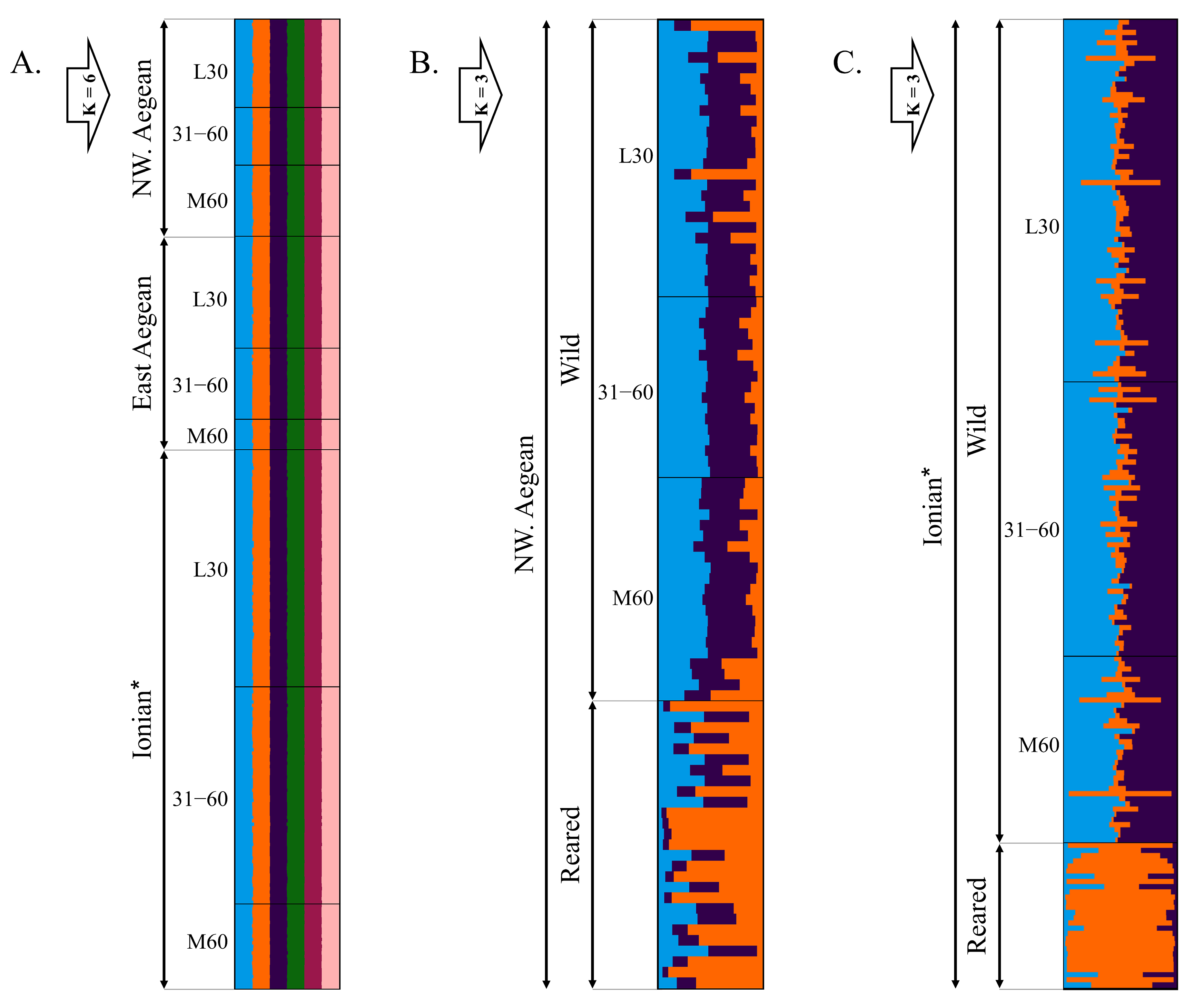
A genetic analysis revealed a higher genetic variation in wild compared to the reared Gilthead seabream populations. In agreement with our results, previous studies that assessed genetic variation using microsatellite markers found similar levels of observed and expected heterozygosity, mean number of alleles, and allelic richness in wild and reared seabream populations throughout Greece [5,14,15,120]. The absence of genetic structuring among the examined seabream samples indicates a genetic homogenization between the Aegean and Ionian Sea populations. Depending on the set of markers used, the existing literature suggests either an absence of genetic structure or a subtle genetic subdivision (FST = 0.009 [5], FST = 0.002 [14]). A recent geographically broad study by Maroso et al. [6] within the Mediterranean Sea and Atlantic Ocean revealed a weak genetic subdivision (FST = 0.007) of wild Gilthead seabreams between the Aegean and Ionian Seas using 1159 genome-wide SNP markers. All these results combined with the absence of discernible physical or ecological barriers along with the long-lasting larval stage of Gilthead seabreams (~50 d [12,19]), enable high dispersal capacity, and support the exchange of individuals between populations of the Aegean and Ionian Seas, ultimately leading to a homogenized genetic pool.
In Greece, there has been an intensive rearing of Gilthead seabreams over the past three decades with rapid expansion in the previous decade [14]. There is a continuous concern that this expansion of aquaculture activity has increased the likelihood of accidental escape events, which could potentially threaten the genetic status of wild fish populations and lead to unknown consequences for their fitness and survival. Reared fish may exhibit large genetic differences from adjacent wild populations mainly due to the different genetic background of broodstocks (i.e., different broodstock origins) or due to the application of selective breeding programs that aim to enhance specific traits [5,15,23]. Our results (FST = 0.014–0.038) are in agreement with the existing literature, which has mainly shown weak genetic divergence between reared and wild Gilthead seabream populations along its distribution range, with FSTs ranging between 0.006–0.069 [3,5,15,18,121,122]. The genetic admixture of escapees with local wild populations could potentially introduce foreign DNA into the wild gene pool and damage local adaptations, but this stands for species with strong genetic structure like salmonids (FST = 0.034–0.2, [123,124,125]). For such species, previous studies have shown that hybrids resulting from crosses between farmed and wild individuals could exhibit lower fitness (e.g., [126]) or relative survival (e.g., [127]) compared to native fish. However, following Sewall Wright’s guideline, FST-values between 0 and 0.05 indicate “no to little genetic differentiation”, FST-values between 0.05 and 0.15 represent moderate differentiation, FST-values between 0.15 and 0.25 are considered large, and FST-values above 0.25 show a very large degree of genetic differentiation [128,129,130,131,132]. It is evident that this is not the case for Gilthead seabreams, which exhibit weak genetic structure with no signs of local adaptations in its populations, mainly due to the high dispersal capability of the species (a long-lived pelagic larval stage [12,19,22]).
Scales have been utilized as a cost-effective and easily applicable morphological trait for identifying aquaculture escapees in the wild. In aquaculture facilities, friction and physical collisions among fish are intensified due to handling manipulations (e.g., counting, size-grading, and vaccination) and high population densities within sea-cages, leading to significantly high rates of scale loss [73,133,134]. Lost scales are promptly replaced by new (regenerated scales), characterized by the presence of a large regeneration nucleus lacking growth circulii [74,135,136]. Based on our results on the otolith shape and asymmetry analyses, fish with a high degree of scale regeneration (31–60 and M60 SRD groups) exhibited increased otolith shape variability in comparison to the L30 group. Furthermore, fish with an M60 SRD exhibited significant differences in otolith shape and higher asymmetry levels compared to other SRD groups. In Gilthead seabreams, reared fish (>94% SRD) display distinct otolith shapes and higher asymmetry levels than wild fish [41]. In addition, Geladakis et al. [41] showed that wild-caught fish with SRD levels greater than 30% exhibit intermediate otolith phenotypes between wild fish with lower SRD (≤30%) and reared fish. Since scales are continuously lost during the rearing process [74], we suggest the 60% SRD as a minimum threshold, beyond which wild-caught fish have an increased possibility of including individuals that escaped from net pens near harvest sizes, thus presenting phenotypes closely similar to those of reared fish. Following our results, a positive correlation emerged between SRD levels and the magnitude of otolith shape and asymmetry variation, suggesting that SRD can not only be used as a reliable index for detecting the presence of aquaculture escapees in the wild, but also to provide insights into the timing of fish escape from aquaculture net pens. On the other hand, a negative correlation was revealed between SRD levels and the genetic diversity (present study). Considering the lower levels of genetic diversity of the reared fish, this is in concordance with the proposal of Geladakis et al. [41,74] that the possibility of the presence of escapees increases as the level of SRD increases, as well. Given the utility of the SRD as a tool for identifying the presence of aquaculture escapees in the wild, the observed variations in SRD levels among wild-caught fish collected across the different years within each geographic group could potentially indicate a transient modification in the proportion of escaped individuals in the wild populations over time.
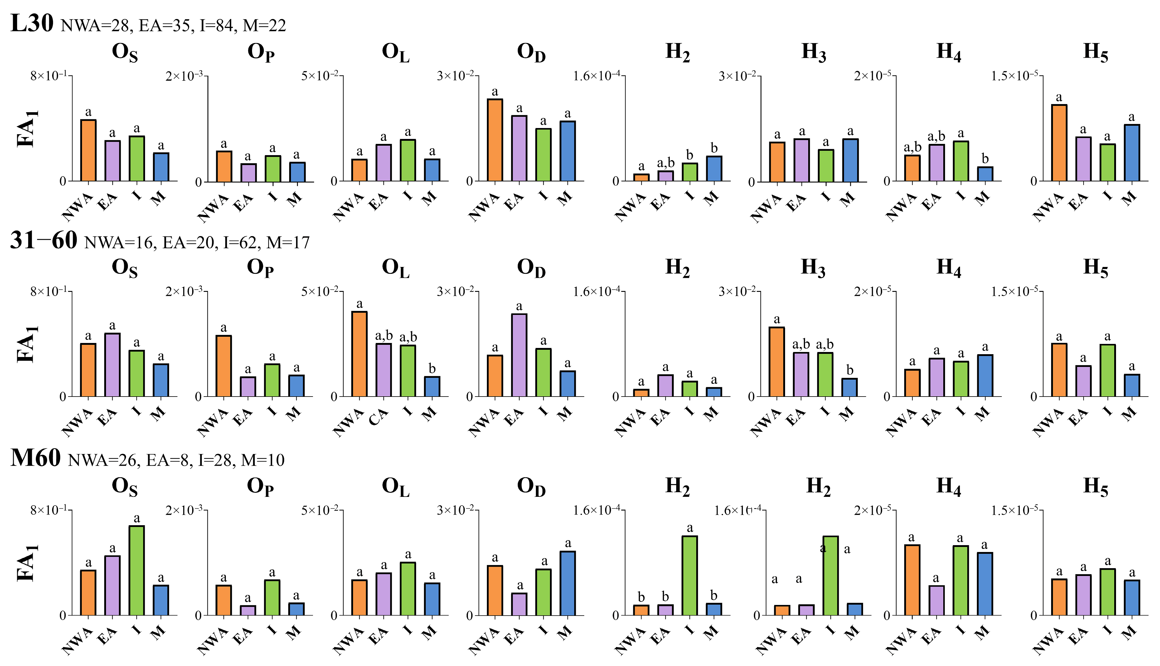
In our study, significant deviations from bilateral symmetry were observed in relation to both the origin within SRD groups and vice versa. These deviations were not restricted to only fluctuating asymmetry (FA), but also included directional asymmetry. Directional asymmetry (DA) refers to a consistent preference of a character toward greater development on one specific body side [137]. In roundfish species, deviations from perfect bilateral symmetry in otolith morphology, expressed as FA or DA, have previously been observed at both early and later stages of fish development (e.g., [41,72,112,113,138,139,140]. Otolith FA is regularly associated with different environmental stressors, and it is considered a sensitive indicator of fish health, performance, and population fitness [65,72]. On the other hand, otolith DA has been suggested to have a genetic origin and/or be a phenotypic plastic response induced by environmental drivers, such as water temperature, indicating a functional adaptation of fish hearing against environmental perturbations [112,113]. In the current work, a spatial variation was observed in the magnitude of otolith asymmetry (expressed as FA or DA) between different geographic groups. Depending on the descriptor examined, in fish with an L30 and 31–60 SRD, the group from Messolonghi lagoon exhibited significantly higher or lower FA or DA compared to other geographic groups. In fish with an L30 SRD, the Ionian group displayed significantly increased otolith shape DA (i.e., in H2 descriptor) compared to the northwestern Aegean fish group. This finding is consistent with a previous study by Mahé et al. [141], which also showed that the amplitude of otolith DA in bogue (Boops boops Linnaeus, 1758) varied geographically, suggesting the potential use of directional bilateral asymmetry in otolith shape as a new method for stock discrimination. The observed shape differences in the right, but not in the left, otolith of the examined wild-caught individuals may be the underlying mechanism of the DA (the right side larger than the left side concerning the shape descriptor H2) induced by early environmental conditions, such as temperature [113]. Bilateral differentiation in the variability of otolith shape was also observed in Mahé et al. [140], with significant discrimination between geographical stock units of bogue with respect to the shape of the right otolith but not the left otolith. However, an open question remains regarding the potential mechanism leading to the bilateral differentiation in otolith biomineralization processes during critical ontogenetic periods of fish and, therefore, the morphological differences between the left and right pair of otoliths.
During the late winter to early spring season (February to March), the Gilthead seabreams from the Ionian Sea temporarily enter the lagoon, which acts as a nursery ground, followed by migration to the open sea for breeding during October to December [76]. The current study indicates that during this brief lagoon period of the Gilthead seabream life cycle, the environmental conditions substantially influence the morphology of their otoliths in terms of both the shape and asymmetry. Coastal lagoons are key ecosystems with increased natural productivity and intensive fishing exploitation by local communities [75]. Fishing activity in these ecosystems is based on the seasonal entrance of young fish in the lagoons, where fish are then captured during their autumn-to-winter offshore migration [76]. The Messolonghi–Etoliko lagoon complex is the largest in Greece and one of the most important coastal lagoon systems in the Mediterranean Sea [142]. Because of the limited depth of the lagoons, meteorological changes rapidly affect the abiotic parameters of the water masses [143]. The interaction between environmental conditions and genetic background could be the underlying mechanisms of otolith shape variability through determination on the relative growth of the different otolith parts (allometry) during fish growth [53,144]. Through the prism of otolith shape plasticity, a brief period of residence in lagoon ecosystems seems to significantly affect the otolith growth trajectories of seabream individuals and, therefore, the resulting otolith morphogenesis.

5. Conclusions

The utilization of diverse methodologies to identify distinct fish stocks enhances our understanding of the attributes that vary among wild populations due to the influence of different environmental and/or genetic factors [31]. Although there is a lack of genetic differentiation among the examined seabream populations, our findings suggest a phenotypic discrimination between the northwestern Aegean and Ionian Gilthead seabream stocks. The combined use of otolith and scale morphology proved to be a useful approach to successfully examine the additive phenotypic variability induced by the presence of aquaculture escapees in the wild seabream stocks.

Supplementary Materials

The following are available online at https://www.mdpi.com/article/10.3390/fishes8060291/s1. Table S1: Sample origin, year and month of collection. n, number of fish analyzed; Table S2: Sampling information per area, year, month and SRD group. n: number of fish analyzed. SLmean: average standard length (±SD, cm); Table S3: Results of pairwise tests (t-tests) for differences in otolith shape between wild-caught fish with different SRD (degree of scale regeneration) levels (Right otolith). L30: wild-caught fish with SRD ≤ 30%; 31–60: fish with SRD 31–60%; M60: fish with SRD > 60%. Number of permutations = 9999. ns, P (perm) > 0.05. * P (perm) < 0.05. ** P (perm) < 0.01. *** P (perm) < 0.001. Number of fish otoliths per group is shown in Table S5; Table S4: Average scores along the first two CAP axes (CAP1, CAP2) for wild-caught fish of different geographical origin. L30: wild-caught fish with SRD (degree of scale regeneration degree) ≤ 30%; 31–60: wild-caught fish with SRD 31–60%; M60: wild-caught fish with SRD > 60%; Table S5: Cross validation re-classification matrix of the canonical analysis of principal coordinates (CAP) on otolith elliptic Fourier data to reclassify wild-caught fish to their origin. L30: wild-caught fish with SRD (degree of scale regeneration) ≤ 30%; 31–60: wild-caught fish with SRD 31–60%; M60: wild-caught fish with SRD > 60%. Different tests were performed for each body side (left, right); Table S6: Summary statistics for genetic variation of Gilthead seabreams per fish group. n: number of fish; A: average number of alleles; Ae: effective number of alleles; Ar: allelic richness; Ho and He: observed and expected heterozygosity; FIS: fixation index. NWA: wild-caught fish from the northwestern Aegean Sea; EA: wild-caught fish from the East Aegean Sea; I: wild-caught fish from both the Ionian Sea and Messolonghi lagoon; L30: wild-caught fish with SRD (degree of scale regeneration) ≤ 30%; 31–60: wild-caught fish with SRD 31–60%; M60: wild-caught fish with SRD > 60%. NWAR: reared fish from the northwestern Aegean Sea; IR: reared fish from the Ionian Sea; Table S7: Pairwise FST (lower triangle) and the respective levels of statistical significance (upper triangle) among wild-caught fish of different geographical origin. L30: wild-caught fish with SRD (degree of scale regeneration) ≤ 30%; 31–60: wild-caught fish with SRD 31–60%; M60: wild-caught fish with SRD > 60%. ns: p > 0.05. Number of fish per group is shown in Table S6; Table S8: Pairwise FST (lower triangle) and the respective levels of statistical significance (upper triangle) among wild-caught fish with different possibility to include aquaculture escapees. L30: wild-caught fish with SRD (degree of scale regeneration) ≤ 30%; 31–60: wild-caught fish with SRD 31–60%; M60: wild-caught fish with SRD > 60%. ns: p > 0.05. Number of fish per group is shown in Table S6; Figure S1: Pie charts illustrating the percentages of wild-caught fish with different SRD (degree of scale regeneration) levels. L30: wild-caught fish with SRD ≤ 30%; 31–60: wild-caught fish with SRD 31–60%; M60: wild-caught fish with SRD > 60%. Number of fish per group is shown in Table 1; Figure S2: Comparison of the index FA1 among wild-caught fish of different SRD (degree of scale regeneration) levels. L30: wild-caught fish with SRD ≤ 30%; 31–60: wild-caught fish with SRD 31–60%; M60: wild-caught fish with SRD > 60%. NWA, northwestern Aegean Sea; EA, East Aegean Sea; I, Ionian Sea; M, Messolonghi lagoon. OL: maximum otolith length; OD: maximum otolith depth; OS: otolith surface area; OP: otolith perimeter; H2-H5: harmonics 2–5. Values without a common letter are statistically different (p < 0.05, F-test). Numerical values next to the geographic groups represent the number of fish otolith pairs per SRD category.

Author Contributions

G.G.: Investigation, Formal analysis, Visualization, Writing—original draft preparation. C.B.: Writing—review and editing, Visualization, Supervision. S.S.: Resources, Writing—review and editing, Visualization, Supervision. G.K.: Conceptualization, Resources, Writing—review and editing, Supervision. All authors have read and agreed to the published version of the manuscript.

Funding

This research received no external funding.

Institutional Review Board Statement

The research conducted in this study exclusively involved fish that were captured and promptly sacrificed either for commercial purposes or as part of experimental sampling efforts conducted by the R/V PHILIA (experimental bottom trawl of Hellenic Centre for Marine Research, HCMR). No live animals were utilized in any capacity during our study. As part of our research, otolith measurements and tissue sampling for DNA extraction concerned fish that had already been sacrificed for commercial or experimental sampling purposes. Consequently, we maintain that obtaining Ethics Committee or Institutional Review Board approval is not necessary for the submission of our manuscript.

Informed Consent Statement

Not applicable.

Data Availability Statement

The data supporting the findings of this study are available from the corresponding authors upon reasonable request.

Acknowledgments

We would like to thank N. Peristeraki, S. Kiparissis and A. Tsikliras for supplying Gilthead seabream samples.

Conflicts of Interest

The authors declare no conflict of interest.

Appendix A

Regarding the left side of the body, in the case of wild-caught individuals with SRD levels ≤ 30% (L30), a selection of m = 32 was determined based on maximum (64.2%) correct reallocations (=35.8% misclassification error, Table S5). The canonical analysis resulted in three canonical axes (the first two are shown, Table S4). The first axis exhibited a squared canonical correlation of δ12 = 0.776 and yielded highly significant permutation statistics (trace statistic = 1.452, p < 0.001, δ12 = 0.776, p < 0.001). For wild-caught individuals with SRD levels between 31–60% (31–60), a choice of m = 22 was determined based on the maximum (58.1%) correct reallocations (=41.9% misclassification error, Table S5). The canonical analysis produced three canonical axes (Table S4), with the first axis demonstrating a squared canonical correlation of δ12 = 0.672 and highly significant permutation statistics (trace statistic = 1.207, p < 0.001, δ12 = 0.672, p < 0.001). Additionally, for wild-caught individuals with an SRD > 60% (M60), a selection of m = 17 was made based on maximum (64.6%) correct reallocations (=35.4% misclassification error, Table S5). The canonical analysis yielded three canonical axes (Table S4), with a squared canonical correlation of the first axis δ12 = 0.657 and highly significant permutation statistics (trace statistic = 1.412, p < 0.001, δ12 = 0.657, p < 0.001).
In the case of the right side of the body, for the fish with an L30 SRD, a selection of m = 23 was made based on the maximum (58.3%) correct reallocations (=41.7% misclassification error, Table S5). The canonical analysis resulted in three canonical axes (Table S4), with the first axis exhibiting a squared canonical correlation of δ12 = 0.454 and highly significant permutation statistics (trace statistic = 0.970, p < 0.001, δ12 = 0.454, p < 0.001). For the fish with a 31–60 SRD, a choice of m = 31 was made based on maximum (65.8%) correct reallocations (=34.2% misclassification error, Table S5). The canonical analysis yielded three canonical axes (Table S4). The first axis demonstrated a squared canonical correlation of δ12 = 0.746 and highly significant permutation statistics (trace statistic = 1.710, p < 0.001, δ12 = 0.746, p < 0.001). Furthermore, for the fish with an M60 SRD, a selection of m = 23 was made based on maximum (60.5%) correct reallocations (=39.5% misclassification error, Table S5). The canonical analysis produced three canonical axes (Table S4), with the first axis demonstrating a squared canonical correlation of δ12 = 0.687 and highly significant permutation statistics (trace statistic = 1.564, p < 0.001, δ12 = 0. 687, p < 0.001).

References

  1. FAO. The State of World Fisheries and Aquaculture 2022. Towards Blue Transformation; FAO: Rome, Italy, 2022. [Google Scholar] [CrossRef]
  2. Bauchot, M.L.; Hureau, J.C. Sparidae. In Check-List of the Fishes of the Eastern Tropical Atlantic (CLOFETA); Quero, J.C., Hureau, J.C., Karrer, C., Post, A., Saldanha, L., Eds.; JNICT: Lisbon, Portugal; SEI: Paris, France; UNESCO: Paris, France, 1990; Volume 2, pp. 790–812. [Google Scholar]
  3. Alarcón, J.A.; Magoulas, A.; Georgakopoulos, T.; Zouros, E.; Alvarez, M.C. Genetic comparison of wild and cultivated european populations of the gilthead sea bream (Sparus aurata). Aquaculture 2004, 230, 65–80. [Google Scholar] [CrossRef]
  4. Funkenstein, B.; Cavari, B.; Stadie, T.; Davidovitch (Yaiche), E. Restriction site polymorphism of mitochondrial DNA of the gilthead sea bream (Sparus aurata) broodstock in Eilat, Israel. Aquaculture 1990, 89, 217–223. [Google Scholar] [CrossRef]
  5. Karaiskou, N.; Triantafyllidis, A.; Katsares, V.; Abatzopoulos, T.J.; Triantaphyllidis, C. Microsatellite variability of wild and farmed populations of Sparus aurata. J. Fish Biol. 2009, 74, 1816–1825. [Google Scholar] [CrossRef]
  6. Maroso, F.; Gkagkavouzis, K.; De Innocentiis, S.; Hillen, J.; do Prado, F.; Karaiskou, N.; Taggart, J.B.; Carr, A.; Nielsen, E.; Triantafyllidis, A.; et al. Genome-wide analysis clarifies the population genetic structure of wild gilthead sea bream (Sparus aurata). PLoS ONE 2021, 16, e0236230. [Google Scholar] [CrossRef]
  7. Palma, J.; Alarcón, J.A.; Alvarez, C.; Zouros, E.; Magoulas, A.; Andrade, J.P. Developmental stability and genetic heterozygosity in wild and cultured stocks of gilthead sea bream (Sparus aurata). J. Mar. Biol. Assoc. UK 2001, 81, 283–288. [Google Scholar] [CrossRef]
  8. Slimen, H.; Guerbej, H.; Othmen, A.; Brahim, I.; Blel, H.; Chatti, N.; Abed, A.; Said, K. Genetic differentiation between populations of gilthead seabream (Sparus aurata) along the Tunisian coast. Cybium 2004, 28, 45–50. [Google Scholar] [CrossRef]
  9. De Innocentiis, S.; Lesti, A.; Livi, S.; Rossi, A.R.; Crosetti, D.; Sola, L. Microsatellite markers reveal population structure in gilthead sea bream Sparus auratus from the Atlantic Ocean and Mediterranean Sea. Fish. Sci. 2004, 70, 852–859. [Google Scholar] [CrossRef]
  10. Rossi, A.R.; Perrone, E.; Sola, L. Genetic structure of gilthead seabream, Sparus aurata, in the Central Mediterranean Sea. Cent. Eur. J. Biol. 2006, 1, 636–647. [Google Scholar] [CrossRef]
  11. Coscia, I.; Vogiatzi, E.; Kotoulas, G.; Tsigenopoulos, C.S.; Mariani, S. Exploring neutral and adaptive processes in expanding populations of gilthead sea bream, Sparus aurata L., in the North-East Atlantic. Heredity 2012, 108, 537–546. [Google Scholar] [CrossRef] [Green Version]
  12. Franchini, P.; Sola, L.; Crosetti, D.; Milana, V.; Rossi, A.R. Low levels of population genetic structure in the gilthead sea bream, Sparus aurata, along the Coast of Italy. ICES J. Mar. Sci. 2012, 69, 41–50. [Google Scholar] [CrossRef] [Green Version]
  13. García-Celdrán, M.; Ramis, G.; María-Dolores, E.; Peñalver, J.; Borrell, Y.J.; Manchado, M.; Estévez, A.; Afonso, J.M.; Armero, E. Genetic assessment of three gilthead sea bream (Sparus aurata L.) populations along the Spanish coast and of three broodstocks managements. Aquac. Int. 2016, 24, 1409–1420. [Google Scholar] [CrossRef]
  14. Gkagkavouzis, K.; Karaiskou, N.; Katopodi, T.; Leonardos, I.; Abatzopoulos, T.J.; Triantafyllidis, A. The genetic population structure and temporal genetic stability of gilthead sea bream Sparus aurata populations in the Aegean and Ionian Seas, using microsatellite DNA markers. J. Fish Biol. 2019, 94, 606–613. [Google Scholar] [CrossRef]
  15. Polovina, E.-S.; Kourkouni, E.; Tsigenopoulos, C.S.; Sanchez-Jerez, P.; Ladoukakis, E.D. Genetic structuring in farmed and wild Gilthead seabream and European seabass in the Mediterranean Sea: Implementations for detection of escapees. Aquat. Living Resour. 2020, 33, 7. [Google Scholar] [CrossRef]
  16. Šegvić-Bubić, T.; Talijančić, I.; Grubišić, L.; Izquierdo-Gomez, D.; Katavić, I. Morphological and molecular differentiation of wild and farmed gilthead sea bream Sparus aurata: Implications for management. Aquac. Environ. Interact. 2014, 6, 43–54. [Google Scholar] [CrossRef] [Green Version]
  17. Šegvić-Bubić, T.; Lepen, I.; Trumbić, Ž.; Ljubković, J.; Sutlović, D.; Matić-Skoko, S.; Grubišić, L.; Glamuzina, B.; Mladineo, I. Population genetic structure of reared and wild gilthead sea bream (Sparus aurata) in the Adriatic Sea inferred with microsatellite loci. Aquaculture 2011, 318, 309–315. [Google Scholar] [CrossRef]
  18. Žužul, I.; Šegvić-Bubić, T.; Talijančić, I.; Džoić, T.; Lepen Pleić, I.; Beg Paklar, G.; Ivatek-Šahdan, S.; Katavić, I.; Grubišić, L. Spatial connectivity pattern of expanding gilthead seabream populations and its interactions with aquaculture sites: A combined population genetic and physical modelling approach. Sci. Rep. 2019, 9, 14718. [Google Scholar] [CrossRef] [Green Version]
  19. Lett, C.; Barrier, N.; Ourmières, Y.; Petit, C.; Labonne, M.; Bourjea, J.; Darnaude, A.M. Modeling Larval Dispersal for the Gilthead Seabream in the Northwestern Mediterranean Sea. Mar. Environ. Res. 2019, 152, 104781. [Google Scholar] [CrossRef] [PubMed] [Green Version]
  20. Moreira, C.; Correia, A.T.; Vaz-Pires, P.; Froufe, E. Genetic Diversity and Population Structure of the Blue Jack Mackerel Trachurus Picturatus across Its Western Distribution. J. Fish Biol. 2019, 94, 725–731. [Google Scholar] [CrossRef] [PubMed]
  21. Correia, A.T.; Faria, R.; Alexandrino, P.; Antunes, C.; Isidro, E.J.; Coimbra, J. Evidence for Genetic Differentiation in the European Conger Eel Conger Conger Based on Mitochondrial DNA Analysis. Fish. Sci. 2006, 72, 20–27. [Google Scholar] [CrossRef]
  22. Shanks, A.L. Pelagic Larval Duration and Dispersal Distance Revisited. Biol. Bull. 2009, 216, 373–385. [Google Scholar] [CrossRef] [Green Version]
  23. Arechavala-Lopez, P.; Toledo-Guedes, K.; Izquierdo-Gomez, D.; Šegvić-Bubić, T.; Sanchez-Jerez, P. Implications of Sea Bream and Sea Bass Escapes for Sustainable Aquaculture Management: A Review of Interactions, Risks and Consequences. Rev. Fish. Sci. Aquac. 2018, 26, 214–234. [Google Scholar] [CrossRef]
  24. Glaropoulos, A.; Papadakis, V.M.; Papadakis, I.E.; Kentouri, M. Escape-related behavior and coping ability of sea bream due to food supply. Aquac. Int. 2012, 20, 965–979. [Google Scholar] [CrossRef]
  25. Dempster, T.; Moe Føre, H.; Fredheim, A.; Jensen, Ø.; Sanchez-Jerez, P. Escapes of marine fish from sea-cage aquaculture in the Mediterranean Sea: Status and prevention. CIESM Work. Monogr. 2007, 32, 55–60. [Google Scholar]
  26. Arechavala-Lopez, P.; Uglem, I.; Fernandez-Jover, D.; Bayle-Sempere, J.T.; Sanchez-Jerez, P. Post-escape dispersion of farmed seabream (Sparus aurata L.) and recaptures by local fisheries in the Western Mediterranean Sea. Fish. Res. 2012, 121–122, 126–135. [Google Scholar] [CrossRef]
  27. Somarakis, S.; Pavlidis, M.; Saapoglou, C.; CS, T.; Dempster, T. Evidence for ‘escape through spawning’ in large gilthead sea bream Sparus aurata reared in commercial sea-cages. Aquac. Environ. Interact. 2013, 3, 135–152. [Google Scholar] [CrossRef] [Green Version]
  28. Arechavala-Lopez, P.; Izquierdo-Gomez, D.; Forcada, A.; Fernandez-Jover, D.; Toledo-Guedes, K.; Valle, C.; Sanchez-Jerez, P. Recapturing fish escapes from coastal farms in the western Mediterranean Sea: Insights for potential contingency plans. Ocean Coast. Manag. 2018, 151, 69–76. [Google Scholar] [CrossRef]
  29. Izquierdo-Gomez, D.; Sanchez-Jerez, P. Management of fish escapes from Mediterranean Sea cage aquaculture through artisanal fisheries. Ocean Coast. Manag. 2016, 122, 57–63. [Google Scholar] [CrossRef]
  30. Toledo-Guedes, K.; Sanchez-Jerez, P.; Brito, A. Influence of a massive aquaculture escape event on artisanal fisheries. Fish. Manag. Ecol. 2014, 21, 113–121. [Google Scholar] [CrossRef]
  31. Begg, G.A.; Waldman, J.R. An holistic approach to fish stock identification. Fish. Res. 1999, 43, 35–44. [Google Scholar] [CrossRef]
  32. Lishchenko, F.; Jones, J.B. Application of Shape Analyses to Recording Structures of Marine Organisms for Stock Discrimination and Taxonomic Purposes. Front. Mar. Sci. 2021, 8, 667183. [Google Scholar] [CrossRef]
  33. Neves, J.; Veríssimo, A.; Múrias Santos, A.; Garrido, S. Comparing Otolith Shape Descriptors for Population Structure Inferences in a Small Pelagic Fish, the European Sardine Sardina Pilchardus (Walbaum, 1792). J. Fish Biol. 2023, 102, 1219–1236. [Google Scholar] [CrossRef] [PubMed]
  34. Ibáñez, A.L.; Hernández-Fraga, K.; Alvarez-Hernández, S. Discrimination Analysis of Phenotypic Stocks Comparing Fish Otolith and Scale Shapes. Fish. Res. 2017, 185, 6–13. [Google Scholar] [CrossRef]
  35. Geladakis, G.; Nikolioudakis, N.; Koumoundouros, G.; Somarakis, S. Morphometric Discrimination of Pelagic Fish Stocks Challenged by Variation in Body Condition. ICES J. Mar. Sci. 2018, 75, 711–718. [Google Scholar] [CrossRef]
  36. Khan, U.; Bal, H.; Battal, Z.S.; Seyhan, K. Using Otolith and Body Shape to Discriminate between Stocks of European Anchovy (Engraulidae: Engraulis Encrasicolus) from the Aegean, Marmara and Black Seas. J. Fish Biol. 2022, 101, 1452–1465. [Google Scholar] [CrossRef] [PubMed]
  37. Muniz, A.A.; Moura, A.; Triay-Portella, R.; Moreira, C.; Santos, P.T.; Correia, A.T. Population Structure of the Chub Mackerel (Scomber Colias) in the North-East Atlantic Inferred from Otolith Shape and Body Morphometrics. Mar. Freshw. Res. 2021, 72, 341–352. [Google Scholar] [CrossRef]
  38. Pawson, M.G.; Jennings, S. A critique of methods for stock identification in marine capture fisheries. Fish. Res. 1996, 25, 203–217. [Google Scholar] [CrossRef]
  39. Arechavala-Lopez, P.; Sanchez-Jerez, P.; Bayle-Sempere, J.T.; Sfakianakis, D.G.; Somarakis, S. Morphological differences between wild and farmed Mediterranean fish. Hydrobiologia 2012, 679, 217–231. [Google Scholar] [CrossRef] [Green Version]
  40. Arechavala-Lopez, P.; Sanchez-Jerez, P.; Bayle-Sempere, J.T.; Sfakianakis, D.G.; Somarakis, S. Discriminating farmed gilthead sea bream Sparus aurata and European sea bass Dicentrarchus labrax from wild stocks through scales and otoliths. J. Fish Biol. 2012, 80, 2159–2175. [Google Scholar] [CrossRef]
  41. Geladakis, G.; Somarakis, S.; Koumoundouros, G. Differences in otolith shape and fluctuating-asymmetry between reared and wild gilthead seabream (Sparus aurata Linnaeus, 1758). J. Fish Biol. 2021, 98, 277–286. [Google Scholar] [CrossRef]
  42. Fragkoulis, S.; Christou, M.; Karo, R.; Ritas, C.; Tzokas, C.; Batargias, C.; Koumoundouros, G. Scaling of body-shape quality in reared gilthead seabream Sparus aurata L. Consumer preference assessment, wild standard and variability in reared phenotype. Aquac. Res. 2017, 48, 2402–2410. [Google Scholar] [CrossRef]
  43. Rogdakis, Y.; Koukou, K.; Ramfos, A.; Dimitriou, E.; Katselis, G. Comparative morphology of wild, farmed and hatchery- released gilthead sea bream (Sparus aurata) in western Greece. Int. Sch. J. 2011, 4, 001–009. [Google Scholar]
  44. Šegvić-Bubić, T.; Talijančić, I.; Vulić, L.; Šegvić, B.; Žužul, I.; Radonić, I.; Grubišić, L. Assignment of Gilthead Seabream Sparus aurata to Its Origin through Scale Shape and Microchemistry Composition: Management Implications for Aquaculture Escapees. Water 2020, 12, 3186. [Google Scholar] [CrossRef]
  45. Talijančić, I.; Šegvić-Bubić, T.; Žužul, I.; Džoić, T.; Maršić-Lučić, J.; Grubišić, L. Morphological and ecophysiological adaptations of wild gilthead seabream Sparus aurata associated with tuna farms. Aquac. Environ. Interact. 2019, 11, 97–110. [Google Scholar] [CrossRef] [Green Version]
  46. Talijančić, I.; Žužul, I.; Kiridžija, V.; Šiljić, J.; Pleadin, J.; Grubišić, L.; Šegvić-Bubić, T. Plastic Responses of Gilthead Seabream Sparus aurata to Wild and Aquaculture Pressured Environments. Front. Mar. Sci. 2021, 8, 694627. [Google Scholar] [CrossRef]
  47. Campana, S.E.; Casselman, J.M. Stock Discrimination Using Otolith Shape Analysis. Can. J. Fish. Aquat. Sci. 1993, 50, 1062–1083. [Google Scholar] [CrossRef]
  48. Campana, S.E.; Neilson, J.D. Microstructure of Fish Otoliths. Can. J. Fish. Aquat. Sci. 1985, 42, 1014–1032. [Google Scholar] [CrossRef]
  49. Panfili, J.; TomÁS, J.; Morales-Nin, B. Otolith Microstructure in Tropical Fish. In Tropical Fish Otoliths: Information for Assessment, Management and Ecology; Green, B.S., Mapstone, B.D., Carlos, G., Begg, G.A., Eds.; Springer Netherlands: Dordrecht, The Netherlands, 2009; pp. 212–248. ISBN 978-1-4020-5775-5. [Google Scholar]
  50. Campana, S.E.; Thorrold, S.R. Otoliths, increments, and elements: Keys to a comprehensive understanding of fish populations? Can. J. Fish. Aquat. Sci. 2001, 58, 30–38. [Google Scholar] [CrossRef]
  51. Cardinale, M.; Doering-Arjes, P.; Kastowsky, M.; Mosegaard, H. Effects of sex, stock, and environment on the shape of known-age Atlantic cod (Gadus morhua) otoliths. Can. J. Fish. Aquat. Sci. 2004, 61, 158–167. [Google Scholar] [CrossRef]
  52. Huang, Y.F.; Song, B.L.; Deng, T.H.; Wang, Q.; Shen, Q.; Liu, L.G. Ontogenetic development, allometric growth patterns, and daily increment validation of larvae and juvenile Culter alburnus. Environ. Biol. Fishes 2021, 104, 1593–1610. [Google Scholar] [CrossRef]
  53. Hüssy, K.; Mosegaard, H.; Albertsen, C.M.; Nielsen, E.E.; Hemmer-Hansen, J.; Eero, M. Evaluation of otolith shape as a tool for stock discrimination in marine fishes using Baltic Sea cod as a case study. Fish. Res. 2016, 174, 210–218. [Google Scholar] [CrossRef] [Green Version]
  54. Mérigot, B.; Letourneur, Y.; Lecomte-Finiger, R. Characterization of local populations of the common sole Solea solea (Pisces, Soleidae) in the NW Mediterranean through otolith morphometrics and shape analysis. Mar. Biol. 2007, 151, 997–1008. [Google Scholar] [CrossRef]
  55. Mille, T.; Mahé, K.; Cachera, M.; Villanueva, M.C.; de Pontual, H.; Ernande, B. Diet is correlated with otolith shape in marine fish. Mar. Ecol. Prog. Ser. 2016, 555, 167–184. [Google Scholar] [CrossRef] [Green Version]
  56. Vignon, M.; Morat, F. Environmental and genetic determinant of otolith shape revealed by a non-indigenous tropical fish. Mar. Ecol. Prog. Ser. 2010, 411, 231–241. [Google Scholar] [CrossRef]
  57. Hoff, N.T.; Dias, J.F.; de Lourdes, Z.-T.M.; Correia, A.T. Spatio-Temporal Evaluation of the Population Structure of the Bigtooth Corvina Isopisthus Parvipinnis from Southwest Atlantic Ocean Using Otolith Shape Signatures. J. Appl. Ichthyol. 2020, 36, 439–450. [Google Scholar] [CrossRef]
  58. Soeth, M.; Daros, F.A.; Correia, A.T.; Fabré, N.N.; Medeiros, R.; Feitosa, C.V.; de Sousa Duarte, O.; Lenz, T.M.; Spach, H.L. Otolith Phenotypic Variation as an Indicator of Stock Structure of Scomberomorus Brasiliensis from the Southwestern Atlantic Ocean. Fish. Res. 2022, 252, 106357. [Google Scholar] [CrossRef]
  59. Castonguay, M.; Simard, P.; Gagnon, P. Usefulness of Fourier Analysis of Otolith Shape for Atlantic Mackerel (Scomber scombrus) Stock Discrimination. Can. J. Fish. Aquat. Sci. 1991, 48, 296–302. [Google Scholar] [CrossRef]
  60. Lombarte, A.; Lleonart, J. Otolith size changes related with body growth, habitat depth and temperature. Environ. Biol. Fishes 1993, 37, 297–306. [Google Scholar] [CrossRef]
  61. Bolles, K.; Begg, G.A. Distinction between silver hake (Merluccius bilinearis) stocks in U.S. waters of the northwest Atlantic based on whole otolith morphometrics. Fish. Bull. 2000, 98, 451–462. [Google Scholar]
  62. Monteiro, L.R.; Di Beneditto, A.P.M.; Guillermo, L.H.; Rivera, L.A. Allometric changes and shape differentiation of sagitta otoliths in sciaenid fishes. Fish. Res. 2005, 74, 288–299. [Google Scholar] [CrossRef]
  63. Hüssy, K. Otolith shape in juvenile cod (Gadus Morhua): Ontogenetic and environmental effects. J. Exp. Mar. Bio. Ecol. 2008, 364, 35–41. [Google Scholar] [CrossRef]
  64. Başusta, N.; Khan, U. Sexual Dimorphism in the Otolith Shape of Shi Drum, Umbrina Cirrosa (L.), in the Eastern Mediterranean Sea: Fish Size–Otolith Size Relationships. J. Fish Biol. 2021, 99, 164–174. [Google Scholar] [CrossRef]
  65. Díaz-Gil, C.; Palmer, M.; Catalán, I.A.; Alós, J.; Fuiman, L.A.; García, E.; del Mar Gil, M.; Grau, A.; Kang, A.; Maneja, R.H.; et al. Otolith fluctuating asymmetry: A misconception of its biological relevance? ICES J. Mar. Sci. 2015, 72, 2079–2089. [Google Scholar] [CrossRef]
  66. Popper, A.N.; Ramcharitar, J.; Campana, S.E. Why Otoliths? Insights from inner ear physiology and fisheries biology. Mar. Freshw. Res. 2005, 56, 497–504. [Google Scholar] [CrossRef]
  67. Ramcharitar, J.U.; Deng, X.; Ketten, D.; Popper, A.N. Form and function in the unique inner ear of a teleost: The silver perch (Bairdiella Chrysoura). J. Comp. Neurol. 2004, 475, 531–539. [Google Scholar] [CrossRef] [PubMed]
  68. Alados, C.L.; Escos, J.; Emlen, J.M. Developmental instability as an indicator of natural stress on the Pacific Hake (Merlussius Productus). Fish. Bull. 1994, 91, 587–593. [Google Scholar]
  69. Somarakis, S.; Kostikas, I.; Peristeraki, N.; Tsimenides, N. Fluctuating asymmetry in the otoliths of larval anchovy Engraulis encrasicolus and the use of developmental instability as an indicator of condition in larval fish. Mar. Ecol. Prog. Ser. 1997, 151, 191–203. [Google Scholar] [CrossRef]
  70. Allenbach, D.M. Fluctuating asymmetry and exogenous stress in fishes: A review. Rev. Fish Biol. Fish. 2011, 21, 355–376. [Google Scholar] [CrossRef]
  71. Fey, D.P.; Hare, J.A. Fluctuating asymmetry in the otoliths of larval Atlantic menhaden Brevoortia tyrannus (Latrobe)–A condition indicator? J. Fish Biol. 2008, 72, 121–130. [Google Scholar] [CrossRef]
  72. Lemberget, T.; McCormick, M.I. Replenishment success linked to fluctuating asymmetry in larval fish. Oecologia 2009, 159, 83–93. [Google Scholar] [CrossRef]
  73. Izquierdo-Gómez, D.; Arechavala-Lopez, P.; Bayle-Sempere, J.T.; Sánchez-Jerez, P. Assessing the influence of gilthead sea bream escapees in landings of Mediterranean fisheries through a scale-based methodology. Fish. Manag. Ecol. 2017, 24, 62–72. [Google Scholar] [CrossRef]
  74. Geladakis, G.; Somarakis, S.; Koumoundouros, G. Scale regeneration in reared Gilthead seabream: Revisiting the use of scales in identifying aquaculture escapees. Aquac. Res. 2021, 52, 4263–4268. [Google Scholar] [CrossRef]
  75. Katselis, G.; Koukou, K.; Dimitriou, E.; Koutsikopoulos, C. Short-term seaward fish migration in the Messolonghi–Etoliko lagoons (Western Greek coast) in relation to climatic variables and the lunar cycle. Estuar. Coast. Shelf Sci. 2007, 73, 571–582. [Google Scholar] [CrossRef]
  76. Katselis, G.; Koutsikopoulos, C.; Dimitriou, E.; Rogdakis, Y. Spatial patterns and temporal trends in the fisheries landings of the Messolonghi-Etoliko lagoons (Western Greek Coast). Sci. Mar. 2003, 67, 501–511. [Google Scholar] [CrossRef] [Green Version]
  77. Costa, M.J.; Cabral, H.N.; Drake, P.; Economou, A.N.; Fernandez-Delgado, C.; Gordo, L.; Marchand, L.; Thiel, R. Recruitment and production of commercial species in estuaries. In Fishes in Estuaries; Elliott, M., Hemingway, K.L., Eds.; Blackwell Science Ltd.: Oxford, UK, 2002; p. 54e123. [Google Scholar]
  78. Quilhac, A.; Sire, J.Y. Restoration of the subepidermal tissues and scale regeneration after wounding a cichlid fish, Hemicromis bimaculatus. J. Exp. Zool. 1998, 281, 305–327. [Google Scholar] [CrossRef]
  79. Schneider, C.A.; Rasband, W.S.; Eliceiri, K.W. NIH Image to ImageJ: 25 Years of image analysis. Nat. Methods 2012, 9, 671–675. [Google Scholar] [CrossRef]
  80. Libungan, L.A.; Pálsson, S. ShapeR: An R Package to Study Otolith Shape Variation among Fish Populations. PLoS ONE 2015, 10, e0121102. [Google Scholar] [CrossRef]
  81. R Core Team. R: A Language and Environment for Statistical Computing; Vienna, Austria: R Foundation for Statistical Computing. 2021. Available online: https://www.R-project.org (accessed on 1 November 2022).
  82. Anderson, M.J. A new method for non-parametric multivariate analysis of variance. Austral Ecol. 2001, 26, 32–46. [Google Scholar] [CrossRef]
  83. Clarke, K.R.; Gorley, R.N. Primer V6: User Manual/Tutorial (Plymouth Routines in Multivariate Ecological Research); Primer-E: Plymouth, UK, 2006. [Google Scholar]
  84. Anderson, M.; Braak, C.T. Permutation tests for multi-factorial analysis of variance. J. Stat. Comput. Simul. 2003, 73, 85–113. [Google Scholar] [CrossRef]
  85. Anderson, M.J.; Willis, T.J. Canonical analysis of principal coordinates: A useful method of constrained ordination for ecology. Ecology 2003, 84, 511–525. [Google Scholar] [CrossRef]
  86. Tort, A. Elliptical Fourier Functions as a Morphological Descriptor of the Genus Stenosarina (Brachiopoda, Terebratulida, New Caledonia). Math. Geol. 2003, 35, 873–885. [Google Scholar] [CrossRef]
  87. Somarakis, S.; Kostikas, I.; Tsimenides, N. Fluctuating asymmetry in the otoliths of larval fish as an indicator of condition: Conceptual and methodological aspects. J. Fish Biol. 1997, 51, 30–38. [Google Scholar] [CrossRef]
  88. Palmer, A.R. Fluctuating asymmetry analyses: A primer. In Developmental Instability: Its Origins and Evolutionary Implications; Markow, T.A., Ed.; Contemporary Issues in Genetics and Evolution: Tempe, AZ, USA, 1994; Volume 2, pp. 335–364. [Google Scholar]
  89. Palmer, A.R.; Strobeck, C. Fluctuating asymmetry as a measure of developmental stability: Implications of non-normal distributions and power of statistical tests. Acta Zool. Fenn. 1992, 191, 55–70. [Google Scholar]
  90. Sokal, R.R.; Rohlf, F.J. Biometry, 2nd ed.; WH Freeman & Co.: New York, NY, USA, 1981. [Google Scholar]
  91. Palmer, A.R.; Strobeck, C. Fluctuating asymmetry: Measurement, analysis, patterns. Annu. Rev. Ecol. Syst. 1986, 17, 391–421. [Google Scholar] [CrossRef]
  92. Walsh, P.S.; Metzger, D.A.; Higuchi, R. Chelex 100 as a Medium for Simple Extraction of DNA for PCR-Based Typing from Forensic Material. Biotechniques 1991, 54, 134–139. [Google Scholar] [CrossRef] [Green Version]
  93. Batargias, C.; Dermitzakis, E.; Magoulas, A.; Zouros, E. Characterization of six polymorphic microsatellite markers in gilthead seabream, Sparus aurata (Linnaeus 1758). Mol. Ecol. 1999, 8, 897–898. [Google Scholar] [PubMed]
  94. Franch, R.; Louro, B.; Tsalavouta, M.; Chatziplis, D.; Tsigenopoulos, C.S.; Sarropoulou, E.; Antonello, J.; Magoulas, A.; Mylonas, C.C.; Babbucci, M.; et al. A Genetic Linkage Map of the Hermaphrodite Teleost Fish Sparus aurata L. Genetics 2006, 174, 851–861. [Google Scholar] [CrossRef] [PubMed] [Green Version]
  95. Sarropoulou, E.; Franch, R.; Louro, B.; Power, D.M.; Bargelloni, L.; Magoulas, A.; Senger, F.; Tsalavouta, M.; Patarnello, T.; Galibert, F.; et al. A gene-based radiation hybrid map of the gilthead sea bream Sparus aurata refines and exploits conserved synteny with Tetraodon nigroviridis. BMC Genom. 2007, 8, 44. [Google Scholar] [CrossRef] [Green Version]
  96. Loukovitis, D.; Sarropoulou, E.; Tsigenopoulos, C.S.; Batargias, C.; Magoulas, A.; Apostolidis, A.P.; Chatziplis, D.; Kotoulas, G. Quantitative Trait Loci Involved in Sex Determination and Body Growth in the Gilthead Sea Bream (Sparus aurata L.) through Targeted Genome Scan. PLoS ONE 2011, 6, e16599. [Google Scholar] [CrossRef] [Green Version]
  97. Toonen, R.; Hughes, S. Increased throughput for fragment analysis on an ABI PRISM 377 automated sequencer using a membrane comb and STRand software. BioTechniques 2001, 31, 1320–1324. [Google Scholar]
  98. Van Oosterhout, C.; Hutchinson, W.F.; Wills, D.P.M.; Shipley, P. Micro-Checker: Software for identifying and correcting genotyping errors in microsatellite data. Mol. Ecol. Notes 2004, 4, 535–538. [Google Scholar] [CrossRef]
  99. ROUSSET, F. Genepop’007: A complete re-implementation of the Genepop Software for Windows and Linux. Mol. Ecol. Resour. 2008, 8, 103–106. [Google Scholar] [CrossRef] [PubMed]
  100. Park, S. MStools v 3.1.1: Excel Spreadsheet Toolkit for Data Conversion. Animal Genomics Lab; University College: Dublin, Ireland, 2008. [Google Scholar]
  101. Yeh, F.C.; Yang, R.C.; Boyle, T.B.J.; Ye, Z.H.; Mao, J.X. PopGene, the User-Friendly Shareware for Population Genetic Analysis, Molecular Biology and Biotechnology Center; University of Alberta: Alberta, EDM, Canada, 1997. [Google Scholar]
  102. Goudet, J. FSTAT, a program to estimate and test gene diversities and differentiation statistics from codominant genetic markers (version 2.9.4). 2003. Available online: https://www2.unil.ch/popgen/softwares/fstat.htm (accessed on 12 December 2022).
  103. Excoffier, L.; Lischer, H.E.L. Arlequin Suite Ver 3.5: A new series of programs to perform population genetics analyses under Linux and Windows. Mol. Ecol. Resour. 2010, 10, 564–567. [Google Scholar] [CrossRef] [PubMed]
  104. Rice, W.R. Analyzing tables of statistical tests. Evolution 1989, 43, 223–225. [Google Scholar] [CrossRef] [PubMed]
  105. Pritchard, J.K.; Stephens, M.; Donnelly, P. Inference of Population Structure Using Multilocus Genotype Data. Genetics 2000, 155, 945–959. [Google Scholar] [CrossRef] [PubMed]
  106. Kopelman, N.M.; Mayzel, J.; Jakobsson, M.; Rosenberg, N.A.; Mayrose, I. Clumpak: A program for identifying clustering modes and packaging population structure inferences across K. Mol. Ecol. Resour. 2015, 15, 1179–1191. [Google Scholar] [CrossRef] [PubMed] [Green Version]
  107. Evanno, G.; Regnaut, S.; Goudet, J. Detecting the number of clusters of individuals using the software Structure: A simulation Study. Mol. Ecol. 2005, 14, 2611–2620. [Google Scholar] [CrossRef] [PubMed] [Green Version]
  108. Rosenberg, N.A. Distruct: A program for the graphical display of population structure. Mol. Ecol. Notes 2004, 4, 137–138. [Google Scholar] [CrossRef]
  109. Vaz-dos-Santos, A.M.; Rautenberg, K.A.; Augusto, C.G.; Ballester, E.L.; Schwingel, P.R.; Pinto, E.; Almeida, A.; Correia, A.T. Geographic Variation in Opisthonema Oglinum (Lesueur, 1818) in the Southeastern Brazilian Bight Inferred from Otolith Shape and Chemical Signatures. Fishes 2023, 8, 234. [Google Scholar] [CrossRef]
  110. Schroeder, R.; Schwingel, P.R.; Correia, A.T. Population Structure of the Brazilian Sardine (Sardinella Brasiliensis) in the Southwest Atlantic Inferred from Body Morphology and Otolith Shape Signatures. Hydrobiologia 2022, 849, 1367–1381. [Google Scholar] [CrossRef]
  111. Vignon, M. Short-term stress for long-lasting otolith morphology—brief embryological stress disturbance can reorient otolith ontogenetic trajectory. Can. J. Fish. Aquat. Sci. 2018, 75, 1713–1722. [Google Scholar] [CrossRef]
  112. Mahé, K.; Gourtay, C.; Defruit, G.B.; Chantre, C.; de Pontual, H.; Amara, R.; Claireaux, G.; Audet, C.; Zambonino-Infante, J.L.; Ernande, B. Do environmental conditions (temperature and food composition) affect otolith shape during fish early-juvenile phase? An experimental approach applied to European Seabass (Dicentrarchus Labrax). J. Exp. Mar. Bio. Ecol. 2019, 521, 151239. [Google Scholar] [CrossRef]
  113. Geladakis, G.; Kourkouta, C.; Somarakis, S.; Koumoundouros, G. Developmental temperature shapes the otolith morphology of metamorphosing and juvenile Gilthead Seabream (Sparus aurata Linnaeus, 1758). Fishes 2022, 7, 82. [Google Scholar] [CrossRef]
  114. Lombarte, A.; Cruz, A. Otolith size trends in marine fish communities from different depth strata. J. Fish Biol. 2007, 71, 53–76. [Google Scholar] [CrossRef]
  115. Volpedo, A.; Echeverria, D.D. Ecomorphological patterns of the sagitta in fish on the continental shelf off Argentine. Fish. Res. 2003, 60, 551–560. [Google Scholar] [CrossRef]
  116. Coll-Lladó, C.; Giebichenstein, J.; Webb, P.B.; Bridges, C.R.; de la Serrana, D.G. Ocean acidification promotes otolith growth and calcite deposition in gilthead sea bream (Sparus aurata) larvae. Sci. Rep. 2018, 8, 8384. [Google Scholar] [CrossRef] [PubMed] [Green Version]
  117. Gagliano, M. Feeding history influences otolith shape in tropical fish. Mar. Ecol. Prog. Ser. 2004, 278, 291–296. [Google Scholar] [CrossRef]
  118. Vasconcelos, J.; Vieira, A.R.; Sequeira, V.; González, J.; Kaufmann, M.; Gordo, L. Identifying Populations of the Blue Jack Mackerel (Trachurus Picturatus) in the Northeast Atlantic by Using Geometric Morphometrics and Otolith Shape Analysis. Fish. Bull. Natl. Ocean. Atmos. Adm. 2018, 116, 81–89. [Google Scholar] [CrossRef] [Green Version]
  119. Capoccioni, F.; Costa, C.; Aguzzi, J.; Menesatti, P.; Lombarte, A.; Ciccotti, E. Ontogenetic and Environmental Effects on Otolith Shape Variability in Three Mediterranean European Eel (Anguilla anguilla, L.) Local Stocks. J. Exp. Mar. Bio. Ecol. 2011, 397, 1–7. [Google Scholar] [CrossRef] [Green Version]
  120. Loukovitis, D.; Sarropoulou, E.; Vogiatzi, E.; Tsigenopoulos, C.S.; Kotoulas, G.; Magoulas, A.; Chatziplis, D. Genetic variation in farmed populations of the gilthead sea bream Sparus aurata in Greece using microsatellite DNA markers. Aquac. Res. 2012, 43, 239–246. [Google Scholar] [CrossRef]
  121. Gkagkavouzis, K.; Papakostas, S.; Maroso, F.; Karaiskou, N.; Carr, A.; Nielsen, E.E.; Bargelloni, L.; Triantafyllidis, A. Investigating Genetic Diversity and Genomic Signatures of Hatchery-Induced Evolution in Gilthead Seabream (Sparus aurata) Populations. Diversity 2021, 13, 563. [Google Scholar] [CrossRef]
  122. Žužul, I.; Grubišić, L.; Šegvić-Bubić, T. Genetic discrimination of wild versus farmed gilthead sea bream Sparus aurata using microsatellite markers associated with candidate genes. Aquat. Living Resour. 2022, 35, 8. [Google Scholar] [CrossRef]
  123. Norris, A.T.; Bradley, D.G.; Cunningham, E.P. Microsatellite genetic variation between and within farmed and wild Atlantic salmon (Salmo salar) populations. Aquaculture 1999, 180, 247–264. [Google Scholar] [CrossRef]
  124. Skaala, Ø.; Høyheim, B.; Glover, K.; Dahle, G. Microsatellite analysis in domesticated and wild Atlantic salmon (Salmo salar L.): Allelic diversity and identification of individuals. Aquaculture 2004, 240, 131–143. [Google Scholar] [CrossRef]
  125. Mjølnerød, I.B.; Refseth, U.H.; Karlsen, E.; Balstad, T.; Jakobsen, K.S.; Hindar, K. Genetic Differences Between Two Wild and One Farmed Population of Atlantic Salmon (Salmo salar) Revealed by Three Classes of Genetic Markers. Hereditas 1997, 127, 239–248. [Google Scholar] [CrossRef]
  126. Reed, T.E.; Prodöhl, P.; Hynes, R.; Cross, T.; Ferguson, A.; McGinnity, P. Quantifying heritable variation in fitness-related traits of wild, farmed and hybrid Atlantic salmon families in a wild river environment. Heredity 2015, 115, 173–184. [Google Scholar] [CrossRef] [Green Version]
  127. Sylvester, E.V.A.; Wringe, B.F.; Duffy, S.J.; Hamilton, L.C.; Fleming, I.A.; Castellani, M.; Bentzen, P.; Bradbury, I.R. Estimating the relative fitness of escaped farmed salmon offspring in the wild and modelling the consequences of invasion for wild populations. Evol. Appl. 2019, 12, 705–717. [Google Scholar] [CrossRef] [Green Version]
  128. Wright, S. Variability within and among natural populations. In Evolution and Genetics of Populations; University of Chicago Press: Chicago, IL, USA, 1978; Volume 4, p. 580. [Google Scholar]
  129. Balloux, F.; Lugon-Moulin, N. The estimation of population differentiation with microsatellite markers. Mol. Ecol. 2002, 11, 155–165. [Google Scholar] [CrossRef] [Green Version]
  130. Tishkoff, S.A.; Kidd, K.K. Implications of biogeography of human populations for ‘race’ and medicine. Nat. Genet. 2004, 36, S21–S27. [Google Scholar] [CrossRef]
  131. Elhaik, E. Empirical Distributions of FST from Large-Scale Human Polymorphism Data. PLoS ONE 2012, 7, e49837. [Google Scholar] [CrossRef] [Green Version]
  132. Bhatia, G.; Patterson, N.; Sankararaman, S.; Price, A.L. Estimating and interpreting FST: The impact of rare variants. Genome Res. 2013, 23, 1514–1521. [Google Scholar] [CrossRef] [Green Version]
  133. LUND, R.A.; HANSEL, L.P. Identification of wild and reared Atlantic salmon, Salmo salar L., using scale characters. Aquac. Res. 1991, 22, 499–508. [Google Scholar] [CrossRef]
  134. Fiske, P.; Lund, R.A.; Hansen, L.P. Identifying fish farm escapees. In Stock Identification Methods: Applications in Fishery Science, 1st ed.; Cardin, S.X., Kerr, L.A., Mariani, S., Eds.; Elsevier Academic Press: Waltham, MA, USA, 2005; pp. 659–680. [Google Scholar]
  135. Bereiter-Hahn, J.; Zylberberg, L. Regeneration of teleost fish scale. Comp. Biochem. Physiol. Part A Physiol. 1993, 105, 625–641. [Google Scholar] [CrossRef]
  136. Blair, A.A. Regeneration of the Scales of Atlantic Salmon. J. Fish. Res. Board Canada 1942, 5c, 440–447. [Google Scholar] [CrossRef]
  137. Palmer, A.R. Waltzing with Asymmetry: Is fluctuating asymmetry a powerful new tool for biologists or just an alluring new dance step? Bioscience 1996, 46, 518–532. [Google Scholar] [CrossRef] [Green Version]
  138. Lychakov, D.V. Behavioral lateralization and otolith asymmetry. J. Evol. Biochem. Physiol. 2013, 49, 441–456. [Google Scholar] [CrossRef]
  139. Mille, T.; Mahé, K.; Villanueva, M.C.; De Pontual, H.; Ernande, B. Sagittal otolith morphogenesis asymmetry in marine fishes. J. Fish Biol. 2015, 87, 646–663. [Google Scholar] [CrossRef]
  140. Mahé, K.; Ider, D.; Massaro, A.; Hamed, O.; Jurado-Ruzafa, A.; Gonçalves, P.; Anastasopoulou, A.; Jadaud, A.; Mytilineou, C.; Elleboode, R.; et al. Directional bilateral asymmetry in otolith morphology may affect fish stock discrimination based on otolith shape analysis. ICES J. Mar. Sci. 2019, 76, 232–243. [Google Scholar] [CrossRef] [Green Version]
  141. Mahé, K.; MacKenzie, K.; Ider, D.; Massaro, A.; Hamed, O.; Jurado-Ruzafa, A.; Gonçalves, P.; Anastasopoulou, A.; Jadaud, A.; Mytilineou, C.; et al. Directional Bilateral Asymmetry in Fish Otolith: A Potential Tool to Evaluate Stock Boundaries? Symmetry 2021, 13, 987. [Google Scholar] [CrossRef]
  142. Dimitriou, E.; Katselis, G.; Moutopoulos, D.K.; Akovitiotis, C.; Koutsikopoulos, C. Possible influence of reared gilthead sea bream (Sparus aurata, L.) on wild stocks in the area of the Messolonghi lagoon (Ionian Sea, Greece). Aquac. Res. 2007, 38, 398–408. [Google Scholar] [CrossRef]
  143. Dimitriou, E.; Athanassopoulos, A.; Kapareliotis, A.; Katselis, G.; Rogdakis, Y.; Betts, H.; Wendling, C. Recordings of the hydrology and fisheries production of on of the fish farms of Messolonghi Etoliko lagoons. In Proceedings of the Ninth Panhellenic Symposium of Ichthyologists, Messolonghi, Greece, 20–23 January 2000. [Google Scholar]
  144. Morales-Nin, B. Review of the growth regulation processes of otolith daily increment formation. Fish. Res. 2000, 46, 53–67. [Google Scholar] [CrossRef]
Figure 1. Map of the sampling area showing the locations of wild-caught fish. (1) Maliakos gulf; (2) Kavala; (3) Kalymnos; (4) Corfu; (5) Central Ionian; (6) Patraikos; (7) Messolonghi lagoon.
Fishes 08 00291 g001
Figure 2. SRD (degree of scale regeneration) frequency distributions of wild-caught fish by geographic group (AD) and regardless of fish origin (E). 2014–2018, sampling years. Number of fish per year for each geographic group is shown in Table S2.
Fishes 08 00291 g002
Figure 3. Plots of scores on the first two CAP axes (CAP1-2) to visualize otolith shape differences among geographic groups. L30: wild-caught fish with degree of scale regeneration (SRD) ≤ 30%; 31–60: fish with SRD 31–60%; M60: fish with SRD > 60%. Number of fish otoliths per group is shown in Table S5.
Fishes 08 00291 g003
Figure 4. Comparison of the index FA1 among wild-caught fish of different geographical origins. NWA, northwestern Aegean Sea; I, Ionian Sea; EA, East Aegean Sea; M, Messolonghi lagoon. L30: wild-caught fish with SRD (degree of scale regeneration) ≤ 30%; 31–60: fish with SRD 31–60%; M60: fish with SRD > 60%. OL: maximum otolith length; OD: maximum otolith depth; OS: otolith surface area; OP: otolith perimeter; H2–H5: harmonics 2–5. Values without a common letter are statistically different (p < 0.05, Bonferroni-corrected F-tests). Numerical values next to the SRD categories represent the number of fish otolith pairs per geographic group.
Fishes 08 00291 g004
Figure 5. Bayesian clustering analysis of Gilthead seabream genotypes at 9 neutral microsatellite loci. (A): all wild-caught fish form six clusters (K = 6); (B,C): reared and wild-caught fish form three clusters (K = 3) for both the northwestern Aegean (NW. Aegean) and Ionian Seas. Black horizontal lines divide individuals belonging to different groups based on their degree of scale regeneration (SRD) and/or based on their wild or reared origin. L30: wild-caught fish with SRD ≤ 30%; 31–60: wild-caught fish with SRD 31–60%; M60: wild-caught fish with SRD > 60%. * Ionian group includes wild-caught fish from both the Ionian Sea and Messolonghi lagoon. Number of fish per group is shown in Table S6.
Fishes 08 00291 g005
Table 1. Characteristics of wild-caught fish samples, classified by their geographic origin and according to their SRD level. n: number of fish; SLmean: average standard length (±SD, cm); SLrange: minimum and maximum standard length; SRD: average degree of scale regeneration (±SD, %). All: all wild-caught fish; L30, wild-caught fish with SRD ≤ 30%; 31–60: wild-caught fish with SRD 31–60%; M60: wild-caught fish with SRD > 60%.
NW. AegeanE. AegeanIonianMessolonghi
Alln756520550
SLmean19.1(2.0)18.4(1.2)17.8(1.9)17.0(0.5)
SLrange13.8–23.715.5–20.913.8–2416.2–18.5
SRD52.7(33.0)34.6(22.1)35.8(23.8)41.6(24.7)
L30n28359922
SLmean17.7(1.9)18.3(1.2)17.4(1.7)17.0(0.4)
SLrange13.8–21.216.4–20.913.8–22.516.3–17.8
SRD17.5(9.0)17.9(9.4)16.7(8.5)18.9(8.9)
31–60n17217117
SLmean19.6(1.3)18.6(1.3)17.8(1.8)17.0(0.5)
SLrange15.8–20.815.5–20.714.2–22.316.2–18.1
SRD46.8(9.8)45.7(7.6)42.0(7.7)48.2(7.9)
M60n3093511
SLmean20.2(1.7)18.3(0.9)18.9(2.1)17.0(0.6)
SLrange15.9–23.716.8–19.813.8–24.016.4–18.5
SRD87.7(12.3)73.6(11.5)77.2(12.3)76.8(12.5)
Table 2. Results of PERMANOVA testing for differences in otolith shape between wild-caught fish of different geographical origins (NW. Aegean, E. Aegean, Ionian, Messolonghi) and SRD levels (L30, 31–60, M60). Different tests were performed for each body side (left, right). Number of permutations = 9999.
OtolithSourceType III Some of SquaresdfMean SquaresPseudo-Fp (perm)
LeftOrigin0.03030.0105.630<0.001
SRD0.00420.0021.1410.296
Origin:SRD0.01560.0031.4530.054
Residuals0.6263570.002
Total0.681368
RightOrigin0.05730.0198.441<0.001
SRD0.00420.0020.9470.471
Origin:SRD0.02360.0041.692<0.01
Residuals0.8053590.002
Total0.887370
Table 3. Results of pairwise tests (t-tests) for differences in otolith shape between fish with different geographical origin (Right otolith). L30: wild-caught fish with SRD (degree of scale regeneration) ≤30%; 31–60: wild-caught fish with SRD 31–60%; M60: wild-caught fish with SRD > 60% Number of permutations = 9999. ns, p (perm) > 0.05. * p (perm) < 0.05. ** p (perm) < 0.01. *** p (perm) < 0.001. Number of fish otoliths per group is shown in Table S5.
L30NW. AegeanE. AegeanIonianMessolonghi
NW. Aegean-*****
E. Aegean1.534-ns***
Ionian1.9921.059-**
Messolonghi2.3372.3272.137-
31–60NW. AegeanE. AegeanIonianMessolonghi
NW. Aegean-********
E. Aegean2.564-ns*
Ionian3.2230.896-**
Messolonghi1.9781.7292.048-
M60NW. AegeanE. AegeanIonianMessolonghi
NW. Aegean-ns***ns
E. Aegean1.303-nsns
Ionian2.0441.117-**
Messolonghi1.3971.3441.866-
Table 4. Estimates of skew (g1) and kurtosis (g2) of otolith asymmetry values (R-L) for surface (OS), perimeter (OP), maximum length (OL), maximum depth (OD), and harmonics 2–5 (H2–H5). SE: standard error, ts: t-statistic, n: sample size. * p < 0.05, ** p < 0.01, *** p < 0.001.
R−LnSkew (g1)Kurtosis (g2)SE (g1)SE (g2)tS (g1)tS (g2)
OS357−0.4172.0740.1290.258−3.23 **8.04 ***
OP357−0.5292.9790.1290.258−4.09 ***11.55 ***
OL357−0.2940.8450.1290.258−2.28 *3.28 **
OD3570.0280.1590.1290.2580.220.62
H23572.24516.1110.1290.25817.37 ***62.48 ***
H33570.0600.9930.1290.2580.473.85 ***
H43570.1161.5530.1290.2580.896.02 ***
H53570.2731.2970.1290.2582.11 *5.03 ***
Table 5. Summary statistics for genetic variation of wild-caught and reared Gilthead seabreams, grouped according to SRD level and expressed as average values among the different geographic regions. n: fish number; A: average number of alleles; Ae: effective number of alleles; Ar: allelic richness; Ho and He: observed and expected heterozygosity; FIS: fixation index. L30: wild-caught fish with SRD (degree of scale regeneration) ≤ 30%; 31–60: wild-caught fish with SRD 31–60%; M60: wild-caught fish with SRD > 60%; NWAR: reared fish from the northwestern Aegean Sea; InR: reared fish from the Ionian Sea.
Fish GroupnAAeArHoHeFIS
L3012914.85 ± 6.098.82 ± 4.828.77 ± 2.660.88 ± 0.020.86 ± 0.03−0.02
31–609113.41 ± 5.528.21 ± 4.138.79 ± 2.780.89 ± 0.020.86 ± 0.03−0.03
M606611.78 ± 5.097.98 ± 4.108.75 ± 2.910.88 ± 0.030.87 ± 0.02−0.02
NWAR2710.44 ± 4.336.46 ± 2.997.39 ± 2.240.84 ± 0.020.83 ± 0.03−0.02
InR289.78 ± 3.65.43 ± 2.437.08 ± 2.030.80 ± 0.030.79 ± 0.03−0.01
Table 6. Pairwise FST (lower triangle) and the respective levels of statistical significance (upper triangle) among reared and wild-caught fish from the northwestern Aegean and the Ionian Sea, respectively. L30: wild-caught fish with SRD (degree of scale regeneration) ≤ 30%; 31–60: wild-caught fish with SRD 31–60%; M60: wild-caught fish with SRD > 60%; ns: p > 0.05, * p < 0.05. Number of fish per group is shown in Table S6.
NW. AegeanL3031–60M60Reared
L30-nsns*
31–600.0027-ns*
M60−0.00720.0016-*
Reared0.01600.01890.0143-
Ionian ¹L3031–60M60Reared
L30-nsns*
31–600.0004-ns*
M600.0003−0.0018-*
Reared0.03990.03950.0374-
¹ Ionian group includes wild-caught fish from both the Ionian Sea and Messolonghi lagoon.
Disclaimer/Publisher’s Note: The statements, opinions and data contained in all publications are solely those of the individual author(s) and contributor(s) and not of MDPI and/or the editor(s). MDPI and/or the editor(s) disclaim responsibility for any injury to people or property resulting from any ideas, methods, instructions or products referred to in the content.

