Article

Climate-Driven Synchrony in Anchovy Fluctuations: A Pacific-Wide Comparison

Institute for Ecological Research and Pollution Control of Plateau Lakes, School of Ecology and Environmental Science, Yunnan University, Kunming 650500, China
*
Author to whom correspondence should be addressed.
Fishes 2022, 7(4), 193; https://doi.org/10.3390/fishes7040193
Submission received: 9 July 2022 / Revised: 2 August 2022 / Accepted: 3 August 2022 / Published: 5 August 2022
(This article belongs to the Special Issue Impacts of Climate Change on Small-Scale Fisheries)

Abstract

:
Fish population fluctuations have been widely documented and are often attributed to climate variability, but little is known about their relationship. This is a barrier that restricts our capacity to understand climate effects on fish fluctuations. Here, we collected published data to conduct a comparative analysis of time series in terms of both scale deposition rate (SDR) and catch to indicate the abundance of anchovy and explored its relationships with climatic and environmental parameters. We first conducted a Spearman correlation analysis to identify the differences in the SDR between sites. Then, we used Generalized Additive Models to evaluate the effects of external forcing at multiple spatial scales (i.e., local and global scales) on the anchovy catches recorded at the California Current Ecosystem (CCE), Humboldt Current Ecosystem (HCE), and Kuroshio Current Ecosystem (KCE). We found that the SDRs at different sites in the same Current Systems are generally consistent, while there are more differences between different systems. We also found that the Pacific Decadal Oscillation index (PDOI), North Pacific index (NPI), North Pacific Gyre Oscillation index (NPGOI), Sea Surface Temperature anomaly (SSTA), and Air Temperature anomaly (ATA) were the most influential factors explaining the variability in anchovy catch for CCE, whereas the NPGOI was the most influential factor for HCE. The PDOI was the best at explaining the variability in anchovy catch for KCE. Our results suggest that anchovy fluctuations in the Pan-Pacific occurred synchronously. These seemingly unrelated events, which occurred thousands of kilometers apart, were actually not isolated. Therefore, we suggest that large-scale climate forcing may activate synchronous fluctuations for anchovy populations at the basin scale, whereas local-scale environmental forces are also responsible for anchovy fluctuations in the “micro-environment”.

1. Introduction

Small pelagic fishes, such as anchovies, sardines, and herrings with an r-selected life history, are short-lived (average 3–7 years) with a high natural mortality. They are also highly mobile, with short, plankton-based food chains [1]. These biological characteristics make their population abundance highly sensitive to environmental stress and make them ideal targets for examining marine ecosystems response to climate variability [2]. Thousand-fold changes have been observed in these fishes abundance in the Pacific since the 1980s [1]. Well-known examples include the sardine, Sardinops sagax, and northern anchovy, Engraulis mordax [3], in the California Current Ecosystem (CCE), the Peruvian anchoveta, Engraulis ringens [4], in the Humboldt Current Ecosystem (HCE), and the Japanese sardine, Sardinops melanostictus, and the Japanese anchovy, Engraulis japonicus [5], in the Kuroshio Current Ecosystem (KCE). In short, their dramatic population fluctuations have important economic, ecological, and social consequences. Therefore, quantitatively identifying the controlling factors for these abnormal changes is of great significance to better understand the trophodynamic processes of food webs, food production in many marine ecosystems, and the population dynamics of small pelagic fishes.
There are eight main species in global anchovy populations: four in the Pacific and four in the Atlantic. The Pacific anchovies differ greatly in terms of life histories and ecological behaviors, with large variances occurring within single species [6]. Anchovies mainly feed on zooplankton and also serve as important prey items for carnivorous fishes at a higher trophic level. They play a critical role in both upward and downward energy transfer in marine food webs [7]. Given their important roles in many marine ecosystems, numerous studies on population fluctuations have been conducted, especially in the upwelling areas [8,9,10]. However, as most former studies focused on investigating fishing rates, limited progress has been achieved in understanding fish fluctuations, due to deficiencies in the length-of-catch data. Fortunately, [11] pioneered the reconstruction of long-term changes in fish abundance based on scale deposition rate (SDR) in the sediments off California. The SDR, as a proxy of fish abundance in historical periods, provides us with a new perspective by which to understand and explore fish fluctuations. Subsequently, innovative work was carried out in multiple regions [3,5,12,13,14], and meaningful results were obtained. Chinese scientists have also adopted the method, implemented it in the central Yellow Sea (YS), and confirmed the feasibility of the method in the Chinese sea [15,16]. On this basis, in combination with biogeochemical proxies, [17] discussed the potential mechanism for anchovy fluctuations in the YS over a 150 yr timescale, suggesting that bottom-up control under climate variability was the main driving force. Furthermore, [18] showed that the bottom-up effect still played a role in anchovy fluctuations over a longer timescale. Nevertheless, data are still needed to understand the mechanisms of fish fluctuations, though some interesting findings have been obtained.
Generally, identifying the variability in anchovy populations and exploring their responses to environmental factors is not only vital to understanding their ecological roles in marine ecosystems but also to improving the robustness of stock assessment and sustainable exploitation. Hence, determining the impacts of environmental factors on fish fluctuations is an urgent need at present. However, much of the knowledge of fish fluctuations is based on correlations that were conducted without a comprehensive understanding. In response to this scientific problem, we first compared the SDR in the YS with available sites in the Pan-Pacific. Then, catch data from CCE, HCE, and KCE were analyzed to investigate the impacts of environmental variables (local-scale) and climate indices (large-scale) on anchovy catch in the Pan-Pacific, and the major driving factors were ultimately identified. Therefore, the purposes of this study are to: (1) clarify the long-term trends in the SDR and anchovy catch at different sites and regions, respectively; (2) identify the climate–environmental controlling factors of anchovy fluctuations; and (3) discuss the possible reasons behind anchovy fluctuations. The results may fill the gaps in the knowledge regarding population dynamics studies of anchovy at a basin scale and could provide suggestions for sustainable anchovy fisheries management around the world.

2. Materials and Methods

2.1. SDR Data

Nine sites were selected for this study, located on the east and the west coasts of the North Pacific and the east coast of the South Pacific, which were affected by California, Kuroshio, and Humboldt currents, respectively (Figure 1). The wind-induced coastal upwellings have obvious impacts on the CCE and HCE at the regional scale, but these impacts are not clear for KCE. Additionally, these sites have distinguishing geographic, oceanographic, and atmospheric conditions. Indeed, all the above differences may induce variability in oceanic conditions in the CCE, HCE, and KCE. All the SDR data used from these sites are as follows: four sites (i.e., Effingham Inlet, Santa Barbara Basin, Guaymas Basin, Soledad Basin) in the CCE of the northeast Pacific; three sites (Callao, Pisco, Mejillones Bay) in the HCE of the southeast Pacific; and two sites (i.e., YS, Beppu Bay) in the KCE of the northwest Pacific. Detailed information is provided in Table 1.

2.2. Catch Data

Obviously, though the length of the systematic catch statistics is shorter than the SDR data, the resolution is higher and is beneficial for further statistical analysis. Hence, in order to explore the links between anchovy and global/local-scale climate–environmental parameters, we also used annual catch data for model analysis. The anchovy catch mainly consisted of two sources for the period of 1950–2015. One was taken from [8], which included the following: northern anchovy in the CCE, the total for Washington, California and Baja California from 1950 to 1996; Peruvian anchoveta in the HCE, the sum of Peru and Chile from 1951 to 1996; in the KCE: Japanese anchovy for China from 1990 to 1996, for Japan from 1950 to 1996, and for Korea from 1950 to 1995. The other database was from FAO FishStatJ database according to country [23] as follows: northern anchovy in the CCE, the total for the USA and Mexico from 1997 to 2015; Peruvian anchoveta in the HCE, the sum of Peru and Chile from 1997 to 2015; in the KCE: Japanese anchovy for China from 1997 to 2015, for Japan from 1997 to 2015, and for Korea (including North and South Korea) from 1996 to 2015.

2.3. Large-Scale Climate Indices

In order to determine the effects of the climate on anchovy fluctuations, we investigated seven climate indices that covered basin-scale environmental conditions. The Pacific Decadal Oscillation index (PDOI), North Pacific index (NPI), North Pacific Gyre Oscillation index (NPGOI), Pacific/North America pattern (PNAP), Southern Oscillation index (SOI), Arctic Oscillation index (AOI), and Monsoon Oscillation index (MOI) were chosen to detect ecological changes in the Pan-Pacific. These basin-scale climate indices are well-documented and largely associated with variations in the Pacific fish populations, communities, and ecosystems [24,25,26,27,28,29]. In general, these indices are more active during the winter [30,31]. Hence, the winter (December–February) average for each index was calculated to represent variability in large-scale teleconnection processes. All indices were derived from open-access online databases for the period from 1950 to 2015. Data descriptions and sources are provided in Table S2 in the Supplementary Material.

2.4. Local-Scale Environmental Variables

Some local-scale environmental variables, such as the Sea Surface Temperature (SST), Air Temperature (AT), Sea Level Pressure (SLP), Sea Surface Salinity (SSS), Scalar Wind (SW), etc., could indicate changes in the hydrodynamic processes for many marine ecosystems. We used ecologically important indicators to measure local-scale climate signals, including the SST, AT, SLP, SSS, and SW to detect local environmental changes in each selected region. It has been extensively reported that variations in the winter average of local-scale environmental variables, as well as basin-scale climate indices, have strong links with variations in various ecological processes [26,30,31,32,33]. Hence, the winter (January–March) average for each variable was calculated to represent variations in the local environmental conditions. All variables were derived from open-access online monthly databases for the period from 1950 to 2015. In this study, the anomalies in all variables were used for further analysis. Detailed descriptions and sources are provided in Table S1 in the Supplementary Material.

2.5. Data Analyses

First, due to the different temporal resolutions among SDR time series in this study, we resampled the data at a 5 yr resolution with a linear interpolation method to make them comparable. Second, as SDR values in the dataset have some zeros, with a non-Gaussian distribution, this limits the use of most parametric methods; thus, we performed a log transformation on the raw data to reduce variability, ensuring the reliability of the results. Third, we calculated Spearman linear correlation coefficients between SDR in the nine sites, with an R package “corrplot” [34]. Fourth, we compared the long-term trends in anchovy catch from three regions (i.e., CCE, HCE, KCE) for the period of 1950–2015. To better explore nonlinear relationships between anchovy catch in these regions with global climate indices and local environmental variables, we finally used the generalized additive models (GAMs) approach with an R package “mgcv” [35]. GAMs are a semi-parametric extension of generalized linear models [36], but they have the advantage of not assuming parametric relations, since the solution is based on smoothing functions that fit the data in a non-linear context [37]. These analyses were conducted either using climate indices or environmental variables separately, or using both with the full model to maximize the proportion of the explained variance, as well as with the best model as determined by the Akaike Information Criterion [38]. All the analyses were performed using the R Software version 4.0.1 (R Project for Statistical Computing).

3. Results

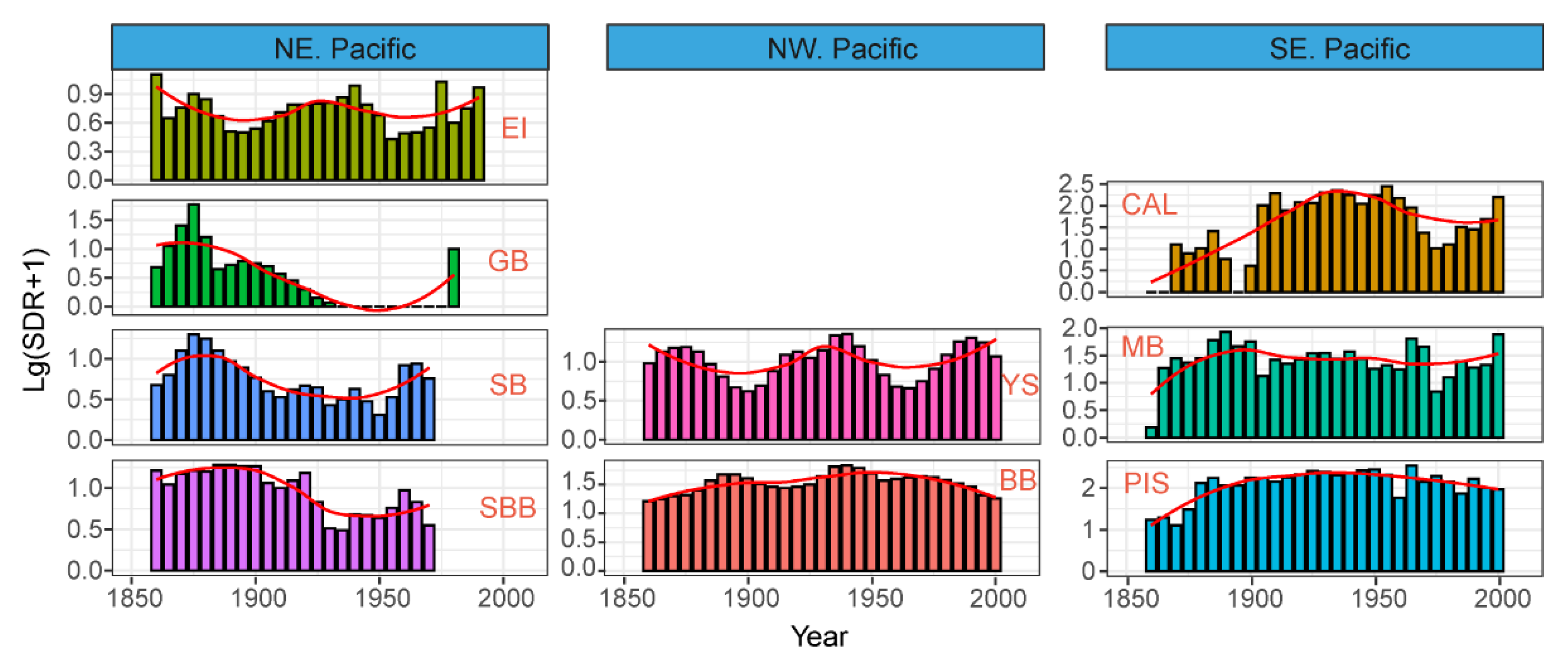
3.1. Major SDR Patterns in the Pan-Pacific

The anchovy SDR showed in-phase or out-of-phase patterns, with different cycles in the Pan-Pacific (Figure 2). Specifically, the SDR fluctuated in-phase for all the sites in the northeast Pacific (CCE) except for the EI (Figure 2); the correlation analysis suggested that EI had no correlation with the other three sites (Figure 3). There was a significant positive correlation between SBB, GB, and SB (Figure 3). The SDR of CAL and PIS showed a positive correlation in the southeast Pacific (HCE) (rs = 0.56, p < 0.05); PIS and BB (KCE) were also positively correlated (rs = 0.61, p < 0.05); and CAL and MB had no correlation (Figure 2 and Figure 3). The SDR in the YS (KCE) showed a clear fluctuation cycle over ~50–60 years, whereas the cycle was not obvious in BB and no clear correlation was found (Figure 2 and Figure 3). Meanwhile, the sites in the SBB, GB, and SB in the northeast Pacific (CCE) were negatively correlated with CAL and PIS in the southeast Pacific (Figure 3). Interestingly, the site in the YS (KCE) was positively correlated with EI in the CCE (rs = 0.71, p < 0.05), but there was no obvious correlation with other sites (Figure 3). Overall, anchovy SDR showed significant multi-decadal fluctuations in the Pan-Pacific.

3.2. Long-Term Changes in Anchovy Catch

As shown in Figure 4, the anchovy catch in the HCE exceeded the rest by almost an order of magnitude. Generally, the anchovy catch showed yearly increases in Korea from 1950 to 2015 (Figure 4e), whereas other catches showed obvious non-stationary fluctuations in manner (Figure 4a–d). Specifically, the relationships between China and other regions (i.e., CCE, HCE, Japan, Korea) were not clear and could be limited by the short length of catch that was studied for China. However, the anchovy catch fluctuated out-of-phase in China and Japan from 1990 to 2015, though they belonged to the northwest Pacific, geographically (Figure 4c,d). Interestingly, the anchovy catch fluctuations were more consistent between HCE and Japan from 1950 to 2015 (Figure 4b,d). CCE and HCE almost showed the opposite trend, especially during the period from 1970 to 1995 (Figure 4a,b).

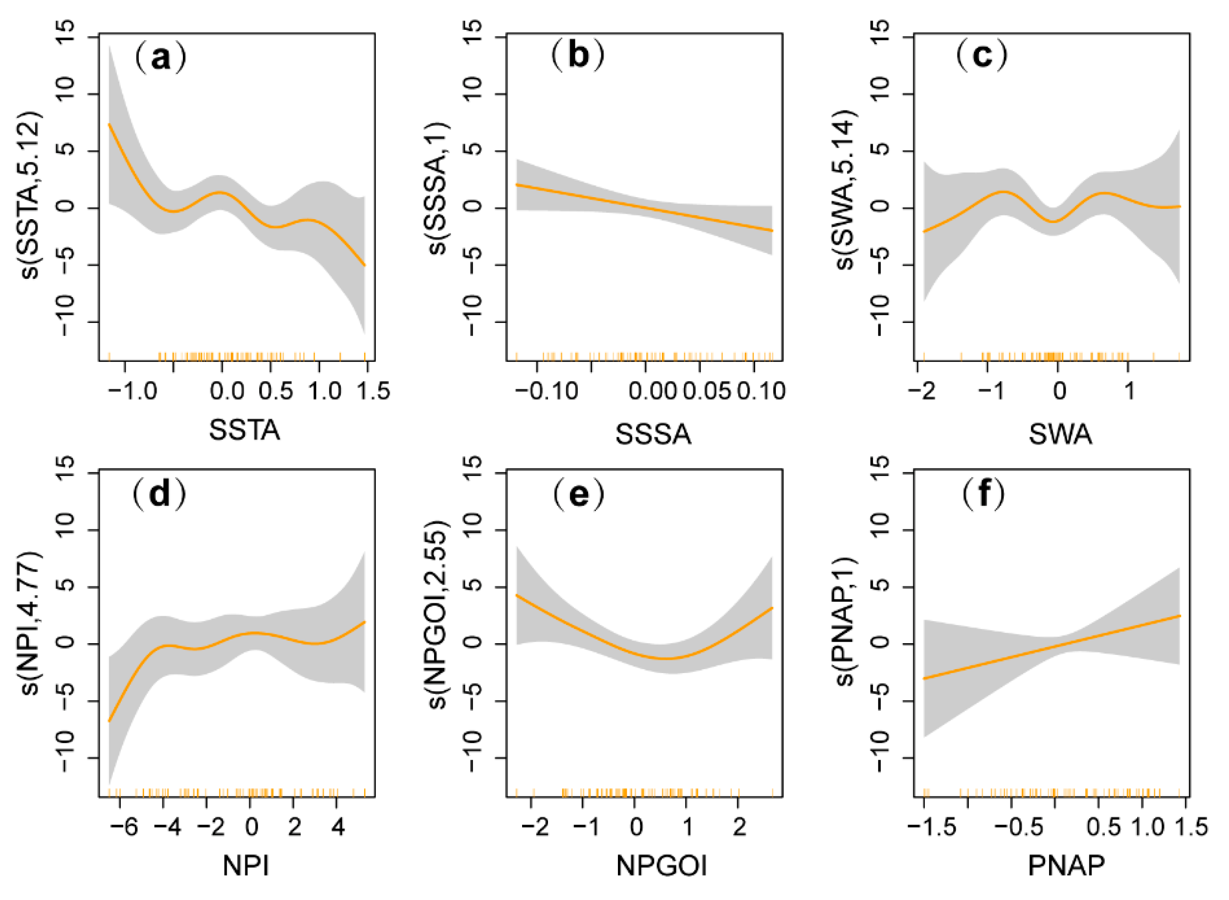
3.3. Results of the GAMs

The results of the GAMs comparing anchovy catch and climate indices and environmental variables are shown in Table S3 in the Supplementary Material. The final GAMs for anchovy catch fit well (deviance explained (DE) = 69% for CCE; DE = 52.9% for HCE; DE = 70% for China; DE = 49.7% for Japan; and DE = 72.8% for Korea). Specifically, anchovy catch in CCE had linear relationships with SSTA, ATA, and PDOI but non-linear relationships with SWA, NPI, and NPGOI (Figure 5). That is, anchovy catch had a negative relationship with SST and positive relationships with AT and PDO (Figure 5a,b,d). It could be seen that moderate SW is beneficial to an increase in anchovy abundance in the CCE (Figure 5c).
Anchovy catch showed a negative relationship with SSSA, a positive relationship with PNAP, and non-linear relationships with SSTA, SWA, NPI, and NPGOI in the HCE (Figure 6). In particular, the relatively low SST and SSS led to an increase in anchovy abundance in the HCE (Figure 6a,b).
In China, anchovy catch showed positive relationships with PDOI, NPGO, and MOI but non-linear relationships with SLPA, SWA, and AOI (Figure 7). Moreover, the relatively low SLP and high SW contributed to an increase in anchovy abundance in Chinese Seas (Figure 7a,b).
Anchovy catch had positive relationships with SSTA, NPGOI, and MOI but non-linear relationships with ATA, SWA, and PDOI in Japan (Figure 8). In particular, the relatively low AT, low SW, and low PDOI were conducive to an increase in anchovy abundance in Japanese waters (Figure 8b–d). GAMs for anchovy catch in both China and Japan had a relatively good performance; however, significant and opposite effects were observed for PDO and SW.
In Korea, anchovy catch had positive relationships with SSTA and AOI, a negative relationship with SWA, and non-linear relationships with SSSA, PDOI, and MOI (Figure 9). In particular, the relatively low SSS, low SW, moderate PDOI, and high MOI led to an increase in anchovy abundance in Korean waters (Figure 9b–d,f). Although MOI had an impact on anchovy in the waters of China, Japan, and Korea in the northwest Pacific, the results were counterintuitive.

4. Discussion

4.1. Consideration of the Method Adopted to Assess the Differences in SDR

In this study, we selected nine sites located in the northeast, southeast, and northwest Pacific, which are affected by California, Humboldt, and Kuroshio currents, respectively. In view of these diversified conditions, there may be a bias in the comparisons of SDR between sites to some extent, which could weaken the reliability of the results. However, the Spearman’s correlation analysis of SDR between sites showed that the uncertainty is moderate. First and foremost, anchovy populations in species unit are closely related to each other in terms of genetics, though they continue to evolve over time and space [6]. Second, all sites were located on Pacific coasts, with a low oxygen concentration and high deposition rate, which ensure an accumulation of fish scales in the sediments. As anchovy was found to be concentrated in the selected areas, these sites could indicate fluctuations in anchovy in abundance [3]. Third, all sites carried out experiments and obtained SDR according to the method described by [11], ensuring the comparability of the data. Finally, we mainly focused on long-term changes instead of specific values in fixed years. Therefore, based on the above reasons, we believe that the results of this study are reliable, though minor effects are inevitable.

4.2. Multiple Modes of Variability in Anchovy Fluctuations

The northern anchovy has three stocks, i.e., northern (Effingham Inlet), central (Santa Barbara Basin), and southern stocks (Guaymas Basin, Soledad Basin) in the CCE [39]. The uneven spatiotemporal distribution of these stocks leads to differences in SDR. Early studies have shown that the cycles of natural fluctuations in anchovy SDR in EI site lasted about 60 years [19], whereas 25–40 years were found for the MB site [13]. Throughout most of the 1970s, the mean anchovy catch in the HCE fell from 12.9 million tons in 1970 to less than 4 million tons, whereas anchovy catch increased in the CCE during the early 1970s, peaked in the 1980s, and then declined in the late 1980s. These out-of-phase fluctuations in anchovy in the HCE and the CCE may be primarily driven by local-scale environmental factors (i.e., SST, SSS for HCE; SST, SW for CCE) rather than fishery regulations. Clearly, anchovy catch showed in-phase fluctuations in the HCE and Japan, which may be largely attributed to large-scale climate forcing [26,40,41]. It is worth noting that the anchovy population in Japan flourished, whereas the anchovy population collapsed in the HCE during warm periods. This may be caused by specific temperature preferences between species [42]. In addition, geographically different hydrological conditions and ocean dynamic processes may be primary causes of these observed fluctuation modes in anchovy.
Although anchovy in the waters of China, Japan, and Korea all belong to the Japanese anchovy in terms of species unit, their population fluctuations show inconsistencies in terms of catch. Although the reasons for this dissimilarity have been debated, they remain inconclusive [14,24]. As the main fishing ground for China and Korea, YS provides the majority of the anchovy catch. The YS is mainly affected by the Yellow Sea warm current, a branch of the Kuroshio current, and the Yellow Sea coastal current. The local oceanic conditions are relatively stable, which may be one of the reasons for the similar trends in anchovy catch in China and Korea. In Japanese waters, local oceanic conditions are more complicated due to the combined effects in the Kuroshio and Oyashio currents, which inevitably produce the reverse trends in anchovy catch in the KCE. Global climate change seems to be the principal force determining the large spatial scale of synchronous anchovy fluctuations across the Pacific [24]. In addition, at the fine spatial scale, there may be differences among regions due to habitat environment and local ecosystem characteristics, resulting in inverted changes in different stocks of the same species [43,44].

4.3. Key Process Affecting Anchovy Fluctuations

The anchovy populations in this study are very separated from each other. Although there are thousands of kilometers in distance between the anchovy populations, they respond to the same basin-wide climate forcing. Therefore, we postulate that anchovy abundance is affected by basin-scale climate forcing in several well-separated regions of the Pacific (i.e., CCE, HCE, KCE). The mechanism driving these anchovy fluctuations is still not well-studied, though some evidence is available. We try to discuss the possible mechanism behind such fluctuation patterns.
Eastern Boundary Current Ecosystems (EBCEs), such as the CCE in the northeast Pacific and the HCE in the southeast Pacific, are the most productive systems on the planet. Although these systems account for less than 1% of the total ocean surface area, they support 20% of global commercial fishery production [45]. The high productivity of these systems depends on wind-driven coastal upwelling, which promotes the growth of phytoplankton by bringing a large amount of nutrient-rich water into the euphotic zone. As a result, with the high nutrients that are available, biological productivity increases, leading to more fish. Intensified coastal upwelling led to increased primary production and fishery yield in the EBCEs [46]. Studies have shown that anchovy is more adapted to high productivity and cool waters of offshore with more zooplankton in the HCE [10,47]. The authors of [4] analyzed the relationship between Peruvian anchoveta and PDO and found that when PDO was in the negative phase, there was low SST with high productivity, resulting in an increase in anchovy abundance. In the CCE, as a result of surface-intensified warming with high SST, the stratification of the water column in the upper ocean increases with deep thermocline and nutrient supply decreases, followed by zooplankton declines [48,49], which leads to a decrease in anchovy abundance. In reality, however, global warming may increase coastal upwelling by strong wind stress and [50], in turn, reduce SST, increase biological productivity, and increase anchovy abundance in the CCE and the HCE. Empirical evidence to support this viewpoint was presented by [51], showing a decline in SST in the CCE and the HCE during 1982–2006 due to strong upwelling. By contrast, the KCE lacks coastal upwelling, but the East Asian monsoon in this region is predominant and can provide similar mechanisms to coastal upwelling. In the KCE of the northwest Pacific, the winter monsoon could affect biological productivity by changing the mixed-layer depth (MLD). That is, a strong winter monsoon brings nutrient-rich water to the euphotic zone, strengthens photosynthesis, increases phytoplankton productivity, and correspondingly induces secondary productivity, thereby supporting abundant fishery production [31,52,53]. Furthermore, due to surface warming and freshening, and strong stratification with shallow MLD, decreased nutrient availability is followed by weakened photosynthesis and reduced marine productivity [54], ultimately affecting fishery yield.
In addition, the GAMs results show that when the PDO is in a positive phase, anchovy abundance significantly increases in CCE and Chinese waters, whereas the opposite effect occurs in Japanese waters, and there is no relationship with anchovy in the HCE. Indeed, in addition to the PDO, the NPGO, and AO also have effects on anchovy in the northwest Pacific (NPGO: China and Japan; AO: Korea). In the CCE and the HCE, the relatively low SST is beneficial to the increase in anchovy, but a low SSS is more helpful to the increase in anchovy in the HCE. In the KCE, a higher SST is conducive to the increase in anchovy in the waters of Japan and Korea. The relatively low SLP and high SW are favorable to the increase in anchovy in Chinese waters, whereas Korea shows the opposite trend. Meanwhile, a growing number of studies have shown that anchovy fluctuations in abundance are directly or indirectly affected by basin-scale climate forcing [10,14,24]. Based on these findings, we suggest that the anchovy fluctuations in the CCE, HCE, and KCE may be generated by bottom-up processes via climate forcing. However, we should not ignore that, because of the existence of local-scale environmental factors, hydrological conditions and ocean dynamic processes vary among different regions. Therefore, considering the effects of the “micro-environment” in each region, to a certain extent, is reasonable when studying how anchovy fluctuations deviate between different regions.

4.4. Broader Implications

In recent decades, fisheries scientists have attempted to distinguish between the two prominent modes (i.e., “bottom-up” control versus “top-down” control). This dichotomy is increasingly considered arbitrary, as the relative importance of each mechanism has been shown to vary over time and space [6,55]. As global warming intensifies, future climate patterns may differ from recent historical periods. Therefore, we need a holistic understanding of the mechanisms based on our increasing knowledge of biogeochemistry, plankton composition and trophic interactions, fish morphology and bioenergetics, and our best prediction of future conditions [6]. The multiple mechanisms involved in fish fluctuations should be given sufficient attention. In particular, the SDR should be further studied in more, and longer, cores in the future to further examine the relationship between anchovy and climate–environmental factors. Traditionally, fishery management mainly focuses on maximizing the catch of a single target species, often neglecting their habitats, predator–prey interactions, and other associated components of the ecosystem. This has some adverse effects on the development of target fishery species. To reduce these negative impacts, an increasing number of scientists are suggesting that some elements of the ecosystem should be fully considered when developing fishery management strategies. The Ecosystem-Based Fishery Management approach fundamentally reverses management priorities from the single target of fish species to ecosystems, with the overall goal of maintaining healthy marine ecosystems and fishery resources [56]. In view of the adverse climate conditions that will occur in the future, anchovy fisheries should be managed in a more cautious manner to maintain their sustainable development and utilization.

5. Conclusions

A century has passed, and the mystery of fish fluctuations remains unsolved. Due to the complexity of marine ecosystems, no single universally applicable theory is adequate to explain the reasons for fish fluctuations, but there may still be a simple and direct mechanism to regulate fish fluctuations at large temporal and spatial scales. Our results suggest that anchovy fluctuations in the Pan-Pacific appear to occur simultaneously. These seemingly unrelated events, thousands of kilometers apart, are not as isolated as they seem. Integrating previous research accumulations, we suggest that large-scale climate forcing may activate synchronous fluctuations in anchovy populations at the basin-scale, while local-scale environmental conditions are also responsible for anchovy fluctuations in the “micro-environment”.

Supplementary Materials

The following supporting information can be downloaded at: https://www.mdpi.com/article/10.3390/fishes7040193/s1, Table S1: Characteristics of local-scale environmental variables used in this study; Table S2: Characteristics of large-scale climate indices used in this study; Table S3: Results of the GAMs between anchovy catch and environmental variables and climate indices. Reference [57] is cited in the supplementary materials

Author Contributions

Conceptualization, validation, supervision, project administration, and funding acquisition, H.Z.; methodology, software, investigation, data curation, visualization, formal analysis, and writing—original draft preparation, H.L.; writing—review and editing, X.Z., Y.Z., Q.L., F.L. and D.L. All authors have read and agreed to the published version of the manuscript.

Funding

This research was funded by the National Natural Science Foundation of China, grant number 41820104008.

Data Availability Statement

The raw data which support this study are available from the corresponding author at reasonable request.

Acknowledgments

We are grateful to S.I. of the Atmosphere and Ocean Research Institute, University of Tokyo, for his helpful comments on and discussions of the early draft of the manuscript. Our acknowledgements are extended to the anonymous reviewers for their constructive suggestions that improved this manuscript.

Conflicts of Interest

All the authors declare no conflict of interest.

References

  1. Alheit, J.; Pohlmann, T.; Casini, M.; Greve, W.; Hinrichs, R.; Mathis, M.; O’Driscoll, K.; Vorberg, R.; Wagner, C. Climate variability drives anchovies and sardines into the North and Baltic Seas. Prog. Oceanogr. 2012, 96, 128–139. [Google Scholar] [CrossRef]
  2. Martín, P.; Sabatés, A.; Lloret, J.; Martin-Vide, J. Climate modulation of fish populations: The role of the Western Mediterranean Oscillation (WeMO) in sardine (Sardina pilchardus) and anchovy (Engraulis encrasicolus) production in the north-western Mediterranean. Clim. Chang. 2012, 110, 925–939. [Google Scholar] [CrossRef]
  3. Baumgartner, T.R.; Soutar, A.; Ferreira-Bartrina, V. Reconstruction of the history of Pacific sardine and northern anchovy populations over the past two millenia from sediments of the Santa Barbara Basin, California. Calif. Coop. Ocean. Fish. 1992, 33, 24–40. [Google Scholar]
  4. Guiñez, M.; Valdés, J.; Sifeddine, A.; Boussafir, M.; Dávila, P.M. Anchovy population and ocean-climatic fluctuations in the Humboldt Current System during the last 700 years and their implications. Palaeogeogr. Palaeoclimatol. Palaeoecol. 2014, 415, 210–224. [Google Scholar] [CrossRef]
  5. Kuwae, M.; Yamamoto, M.; Sagawa, T.; Ikehara, K.; Irino, T.; Takemura, K.; Takeoka, H.; Sugimoto, T. Multidecadal, centennial, and millennial variability in sardine and anchovy abundances in the western North Pacific and climate–fish linkages during the late Holocene. Prog. Oceanogr. 2017, 159, 86–98. [Google Scholar] [CrossRef]
  6. Checkley, D.M.; Asch, R.G.; Rykaczewski, R.R. Climate, Anchovy, and Sardine. Ann. Rev. Mar. Sci. 2017, 9, 469–493. [Google Scholar] [CrossRef] [Green Version]
  7. MacCall, A.D. Mechanisms of low-frequency fluctuations in sardine and anchovy populations. In Climate Change and Small Pelagic Fish; Checkley, D., Alheit, J., Oozeki, Y., Roy, C., Eds.; Cambridge University Press: Cambridge, UK, 2009; pp. 285–299. [Google Scholar]
  8. Schwartzlose, R.A.; Alheit, J.; Bakun, A.; Baumgartner, T.R.; Cloete, R.; Crawford, R.J.M.; Fletcher, W.J.; Green-Ruiz, Y.; Hagen, E.; Kawasaki, T.; et al. Worldwide large-scale fluctuations of sardine and anchovy populations. S. Afr. J. Mar. Sci. 1999, 21, 289–347. [Google Scholar] [CrossRef]
  9. McClatchie, S.; Hendy, I.L.; Thompson, A.R.; Watson, W. Collapse and recovery of forage fish populations prior to commercial exploitation. Geophys. Res. Lett. 2017, 44, 1877–1885. [Google Scholar] [CrossRef]
  10. Salvatteci, R.; Field, D.; Gutierrez, D.; Baumgartner, T.; Ferreira, V.; Ortlieb, L.; Sifeddine, A.; Grados, D.; Bertrand, A. Multifarious anchovy and sardine regimes in the Humboldt Current System during the last 150 years. Glob. Chang. Biol. 2018, 24, 1055–1068. [Google Scholar] [CrossRef]
  11. Soutar, A.; Isaacs, J.D. History of fish populations inferred from fish scales in anaerobic sediments off California. Calif. Coop. Ocean. Fish. 1969, 13, 63–70. [Google Scholar]
  12. Wright, C.A.; Dallimore, A.; Thomson, R.E.; Patterson, R.T.; Ware, D.M. Late Holocene paleofish populations in Effingham Inlet, British Columbia, Canada. Palaeogeogr. Palaeoclimatol. Palaeoecol. 2005, 224, 367–384. [Google Scholar] [CrossRef]
  13. Valdés, J.; Ortlieb, L.; Gutierrez, D.; Marinovic, L.; Vargas, G.; Sifeddine, A. 250 years of sardine and anchovy scale deposition record in Mejillones Bay, northern Chile. Prog. Oceanogr. 2008, 79, 198–207. [Google Scholar] [CrossRef]
  14. Zhou, X.; Sun, Y.; Huang, W.; Smol, J.P.; Tang, Q.; Sun, L. The Pacific decadal oscillation and changes in anchovy populations in the Northwest Pacific. J. Asian. Earth. Sci. 2015, 114, 504–511. [Google Scholar] [CrossRef]
  15. Jia, H.; Sun, Y.; Zhao, M.; Yang, Z.; Tang, Q. Fish-scale-deposition information and spatial distribution in typical fishery area of the Yellow Sea and East China Sea. J. Fish. China 2008, 32, 584–591. [Google Scholar]
  16. Huang, J.; Sun, Y.; Jia, H.; Tang, Q. Last 150-Year Variability in Japanese Anchovy (Engraulis japonicus) Abundance Based on the Anaerobic Sediments of the Yellow Sea Basin in the Western North Pacific. J. Ocean. Univ. China 2016, 15, 131–136. [Google Scholar] [CrossRef]
  17. Li, H.; Tang, Q.; Ito, S.-I.; Sun, Y. Evidence of bottom-up effects of climate on Japanese anchovy (Engraulis japonicus) in the western North Pacific. J. Oceanogr. 2021, 77, 589–605. [Google Scholar] [CrossRef]
  18. Li, H.; Tang, Q.; Sun, Y. Response of Japanese anchovy (Engraulis japonicus) to the Pacific Decadal Oscillation in the Yellow Sea over the past 400 a. Acta Oceanol. Sin. 2022; in press. [Google Scholar] [CrossRef]
  19. Holmgren, D. Decadel-Centennial Variability in Marine Ecosystem of the Northeast Pacific Ocean: The Use of Fish Scales Deposition in Sediments; University of Washington: Washington, DC, USA, 2001. [Google Scholar]
  20. Soutar, A.; Isaacs, J.D. Abundance of pelagic fish during the 19th and 20th centuries as recorded in anaerobic sediment off the Californias. Fish. Bull. 1974, 72, 257–273. [Google Scholar]
  21. Holmgren-Urba, D.; Baumgartner, T.R. A 250-year history of pelagic fish abundances from the anaerobic sediments of the central Gulf of California. Calif. Coop. Ocean. Fish. 1993, 34, 60–68. [Google Scholar]
  22. Gutiérrez, D.; Sifeddine, A.; Field, D.B.; Ortlieb, L.; Vargas, G.; Chávez, F.P.; Velazco, F.; Ferreira, V.; Tapia, P.; Salvatteci, R.; et al. Rapid reorganization in ocean biogeochemistry off Peru towards the end of the Little Ice Age. Biogeosciences 2009, 6, 835–848. [Google Scholar] [CrossRef] [Green Version]
  23. FAO. Fishery and Aquaculture Statistics. In Global Capture Production 1950–2015 (FishstatJ); FAO: Rome, Italy, 2017. [Google Scholar]
  24. Chavez, F.P.; Ryan, J.; Lluch-Cota, S.E.; Ñiquen, C.M. From Anchovies to Sardines and Back: Multidecadal Change in the Pacific Ocean. Science 2003, 299, 217–221. [Google Scholar] [CrossRef] [PubMed] [Green Version]
  25. Di Lorenzo, E.; Schneider, N.; Cobb, K.M.; Franks, P.J.S.; Chhak, K.; Miller, A.J.; McWilliams, J.C.; Bograd, S.J.; Arango, H.; Curchitser, E.; et al. North Pacific Gyre Oscillation links ocean climate and ecosystem change. Geophys. Res. Lett. 2008, 35, L08607. [Google Scholar] [CrossRef] [Green Version]
  26. Alheit, J.; Bakun, A. Population synchronies within and between ocean basins: Apparent teleconnections and implications as to physical–biological linkage mechanisms. J. Mar. Syst. 2010, 79, 267–285. [Google Scholar] [CrossRef]
  27. Litzow, M.A.; Mueter, F.J.; Hobday, A.J. Reassessing regime shifts in the North Pacific: Incremental climate change and commercial fishing are necessary for explaining decadal-scale biological variability. Glob. Chang. Biol. 2014, 20, 38–50. [Google Scholar] [CrossRef]
  28. Litzow, M.A.; Ciannelli, L.; Puerta, P.; Wettstein, J.J.; Rykaczewski, R.R.; Opiekun, M. Non-stationary climate–salmon relationships in the Gulf of Alaska. Proc. Royal Soc. B. 2018, 285, 20181855. [Google Scholar] [CrossRef] [Green Version]
  29. Litzow, M.A.; Malick, M.J.; Bond, N.A.; Cunningham, C.J.; Gosselin, J.L.; Ward, E.J. Quantifying a Novel Climate Through Changes in PDO-Climate and PDO-Salmon Relationships. Geophys. Res. Lett. 2020, 47, e2020GL087972. [Google Scholar] [CrossRef]
  30. Ma, S.; Liu, Y.; Li, J.; Fu, C.; Ye, Z.; Sun, P.; Yu, H.; Cheng, J.; Tian, Y. Climate-induced long-term variations in ecosystem structure and atmosphere-ocean-ecosystem processes in the Yellow Sea and East China Sea. Prog. Oceanogr. 2019, 175, 183–197. [Google Scholar] [CrossRef]
  31. Jung, H.K.; Rahman, S.M.M.; Kang, C.-K.; Park, S.-Y.; Heon Lee, S.; Je Park, H.; Kim, H.-W.; Lee, C.I. The influence of climate regime shifts on the marine environment and ecosystems in the East Asian Marginal Seas and their mechanisms. Deep Sea Res. Part II Top. Stud. Oceanogr. 2017, 143, 110–120. [Google Scholar] [CrossRef]
  32. Overland, J.E.; Alheit, J.; Bakun, A.; Hurrell, J.W.; Mackas, D.L.; Miller, A.J. Climate controls on marine ecosystems and fish populations. J. Mar. Syst. 2010, 79, 305–315. [Google Scholar] [CrossRef]
  33. Ma, S.; Tian, Y.; Fu, C.; Yu, H.; Li, J.; Liu, Y.; Cheng, J.; Wan, R.; Watanabe, Y. Climate-induced nonlinearity in pelagic communities and non-stationary relationships with physical drivers in the Kuroshio ecosystem. Fish Fish. 2020, 22, 1–17. [Google Scholar] [CrossRef]
  34. Wei, T.; Simko, V. R Package “Corrplot”: Visualization of a Correlation Matrix, Version 0.84. 2017.
  35. Wood, S.N. Generalized Additive Models: An Introduction with R, 2nd ed.; Chapman and Hall/CRC: New York, NY, USA, 2017; p. 496. [Google Scholar]
  36. Hastie, T.J.; Tibshirani, R.J. Monographs on Statistics and Applied Probability in Generalized Linear Models; Chapman & Hall: London, UK, 1990; Volume 43, pp. 205–208. [Google Scholar]
  37. Zuur, A.; Ieno, E.N.; Smith, G.M. Analyzing Ecological Data; Springer: New York, NY, USA, 2007; p. 672. [Google Scholar]
  38. Vrieze, S.I. Model selection and psychological theory: A discussion of the differences between the Akaike information criterion (AIC) and the Bayesian information criterion (BIC). Psychol. Methods 2012, 17, 228–243. [Google Scholar] [CrossRef] [Green Version]
  39. McHugh, J.L. Meristic Variations and Populations of Northern Anchovy (Engraulis Mordax Mordax). Scripps Inst. Oceanogr. Bull. 1951, 6, 123–160. [Google Scholar] [CrossRef]
  40. Oozeki, Y.; Ñiquen Carranza, M.; Takasuka, A.; Ayón Dejo, P.; Kuroda, H.; Tam Malagas, J.; Okunishi, T.; Vásquez Espinoza, L.; Gutiérrez Aguilar, D.; Okamura, H.; et al. Synchronous multi-species alternations between the northern Humboldt and Kuroshio Current systems. Deep Sea Res. Part II Top. Stud. Oceanogr. 2019, 159, 11–21. [Google Scholar] [CrossRef]
  41. Izquierdo-Peña, V.; Lluch-Cota, S.E.; Hernandez-Rivas, M.E.; Martínez-Rincón, R.O. Revisiting the Regime Problem hypothesis: 25 years later. Deep Sea Res. Part II Top. Stud. Oceanogr. 2019, 159, 4–10. [Google Scholar] [CrossRef]
  42. Takasuka, A.; Oozeki, Y.; Kubota, H.; Lluch-Cota, S.E. Contrasting spawning temperature optima: Why are anchovy and sardine regime shifts synchronous across the North Pacific? Prog. Oceanogr. 2008, 77, 225–232. [Google Scholar] [CrossRef]
  43. Hilborn, R.; Quinn, T.P.; Schindler, D.E.; Rogers, D.E. Biocomplexity and fisheries sustainability. Proc. Natl. Acad. Sci. USA 2003, 100, 6564–6568. [Google Scholar] [CrossRef] [Green Version]
  44. Rogers, L.A.; Schindler, D.E.; Lisi, P.J.; Holtgrieve, G.W.; Leavitt, P.R.; Bunting, L.; Finney, B.P.; Selbie, D.T.; Chen, G.; Gregory-Eaves, I.; et al. Centennial-scale fluctuations and regional complexity characterize Pacific salmon population dynamics over the past five centuries. Proc. Natl. Acad. Sci. USA 2013, 110, 1750–1755. [Google Scholar] [CrossRef] [Green Version]
  45. Pauly, D.; Christensen, V. Primary production required to sustain global fisheries. Nature 1995, 374, 255–257. [Google Scholar] [CrossRef]
  46. Rykaczewski, R.R.; Checkley, D.M. Influence of ocean winds on the pelagic ecosystem in upwelling regions. Proc. Natl. Acad. Sci. USA 2008, 105, 1965–1970. [Google Scholar] [CrossRef] [Green Version]
  47. Ayón, P.; Swartzman, G.; Bertrand, A.; Gutiérrez, M.; Bertrand, S. Zooplankton and forage fish species off Peru: Large-scale bottom-up forcing and local-scale depletion. Prog. Oceanogr. 2008, 79, 208–214. [Google Scholar] [CrossRef]
  48. Roemmich, D.; McGowan, J. Climatic Warming and the Decline of Zooplankton in the California Current. Science 1995, 267, 1324–1326. [Google Scholar] [CrossRef] [PubMed]
  49. Fiechter, J.; Rose, K.A.; Curchitser, E.N.; Hedstrom, K.S. The role of environmental controls in determining sardine and anchovy population cycles in the California Current: Analysis of an end-to-end model. Prog. Oceanogr. 2015, 138, 381–398. [Google Scholar] [CrossRef] [Green Version]
  50. Bakun, A. Global climate change and intensification of coastal ocean upwelling. Science 1990, 247, 198–201. [Google Scholar] [CrossRef] [PubMed] [Green Version]
  51. Belkin, I.M. Rapid warming of Large Marine Ecosystems. Prog. Oceanogr. 2009, 81, 207–213. [Google Scholar] [CrossRef]
  52. Yatsu, A.; Chiba, S.; Yamanaka, Y.; Ito, S.I.; Shimizu, Y.; Kaeriyama, M.; Watanabe, Y. Climate forcing and the Kuroshio/Oyashio ecosystem. ICES J. Mar. Sci. 2013, 70, 922–933. [Google Scholar] [CrossRef] [Green Version]
  53. Hollowed, A.B.; Barange, M.; Beamish, R.J.; Brander, K.; Cochrane, K.; Drinkwater, K.; Foreman, M.G.G.; Hare, J.A.; Holt, J.; Ito, S.-i.; et al. Projected impacts of climate change on marine fish and fisheries. ICES J. Mar. Sci. 2013, 70, 1023–1037. [Google Scholar] [CrossRef] [Green Version]
  54. Jang, C.J.; Park, J.; Park, T.; Yoo, S. Response of the ocean mixed layer depth to global warming and its impact on primary production: A case for the North Pacific Ocean. ICES J. Mar. Sci. 2011, 68, 996–1007. [Google Scholar] [CrossRef] [Green Version]
  55. Lynam, C.P.; Llope, M.; Möllmann, C.; Helaouët, P.; Bayliss-Brown, G.A.; Stenseth, N.C. Interaction between top-down and bottom-up control in marine food webs. Proc. Natl. Acad. Sci. USA 2017, 114, 1952–1957. [Google Scholar] [CrossRef] [Green Version]
  56. Pikitch, E.K.; Santora, C.; Babcock, E.A.; Bakun, A.; Bonfil, R.; Conover, D.O.; Dayton, P.; Doukakis, P.; Fluharty, D.; Heneman, B.; et al. Ecosystem-Based Fishery Management. Science 2004, 305, 346–347. [Google Scholar] [CrossRef]
  57. Tian, Y.; Kidokoro, H.; Watanabe, T.; Iguchi, N. The late 1980s regime shift in the ecosystem of Tsushima warm current in the Japan/East Sea: Evidence from historical data and possible mechanisms. Prog. Oceanogr. 2008, 77, 127–145. [Google Scholar] [CrossRef]
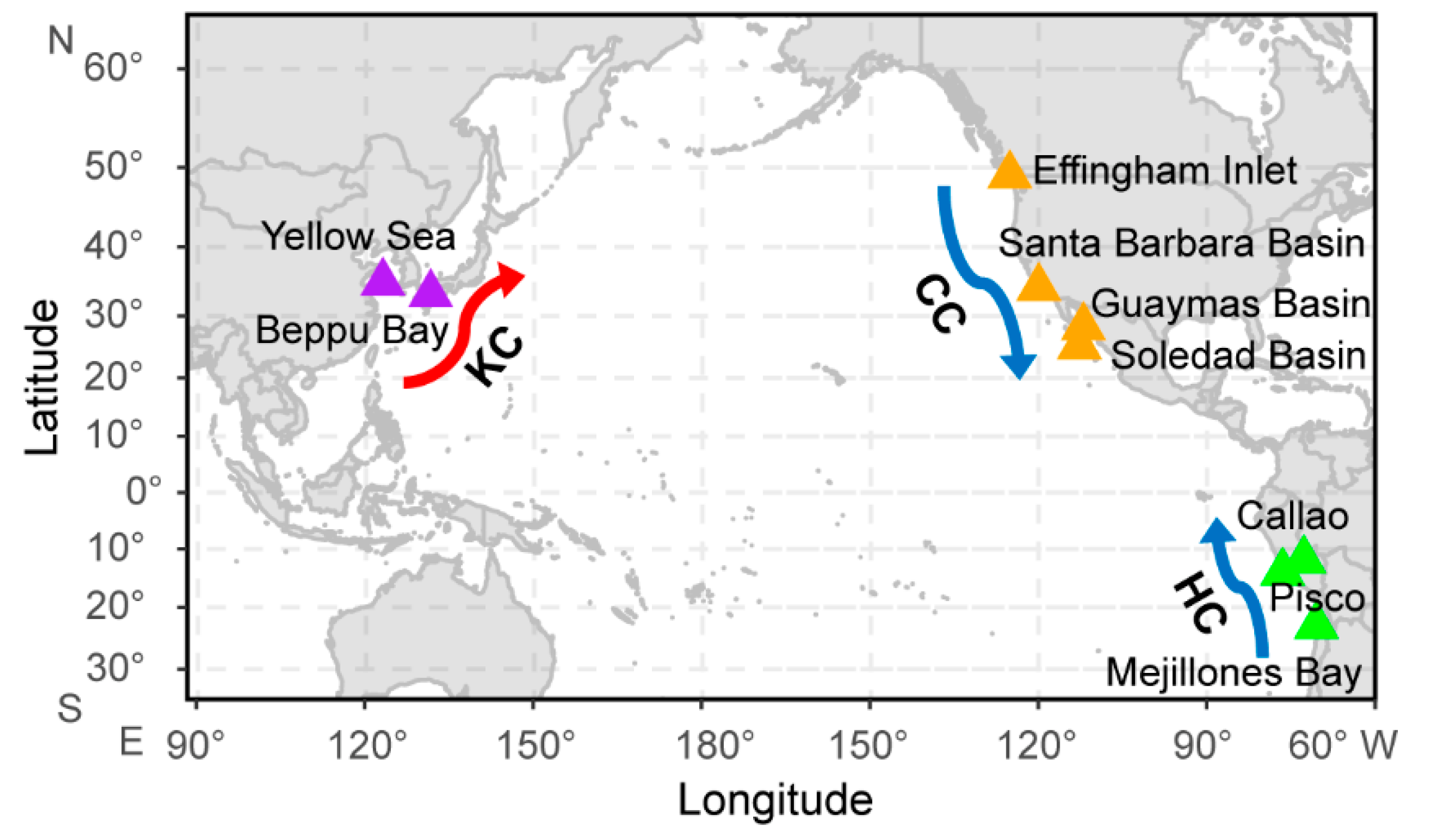
Figure 1. The map of research sites in the Pan-Pacific. Arrows represent the ocean currents. Warm current (red): Kuroshio Current (KC); cold currents (blue): California and Humboldt Currents (CC and HC).
Fishes 07 00193 g001
Figure 2. Long-term changes in the SDR from sites in the Pan-Pacific. SDR: scale deposition rate (#scales cm−2 yr−1). Red lines represent the smooth curve with a loess method. YS: Yellow Sea; BB: Beppu Bay; EI: Effingham Inlet; SBB: Santa Barbara Basin; GB: Guaymas Basin; SB: Soledad Basin; CAL: Callao; PIS: Pisco; MB: Mejillones Bay.
Fishes 07 00193 g002
Figure 3. Spearman’s correlation matrix in the scale deposition rate (SDR) from sites in the Pan-Pacific. The numbers indicate value of correlation coefficient, and the red X shows that the significance test of p < 0.05 failed. YS: Yellow Sea; BB: Beppu Bay; EI: Effingham Inlet; SBB: Santa Barbara Basin; GB: Guaymas Basin; SB: Soledad Basin; CAL: Callao; PIS: Pisco; MB: Mejillones Bay.
Fishes 07 00193 g003
Figure 4. Long-term changes in anchovy catch in the Pan-Pacific. (ae) Anchovy catch in the CCE, HCE, CHN, JAP, and KOR, respectively. CCE: California Current Ecosystem; HCE: Humboldt Current Ecosystem; CHN: China; JAP: Japan; KOR: Korea. The vertical dashed line indicates the boundary values of the [8,23], respectively.
Fishes 07 00193 g004
Figure 5. Generalized additive models (GAMs) between anchovy catch and environmental variables and climate indices in the California Current Ecosystem (CCE). (a) Anchovy versus Sea Surface Temperature anomaly (SSTA). (b) Anchovy versus Air Temperature anomaly (ATA). (c) Anchovy versus Scalar Wind anomaly (SWA). (d) Anchovy versus Pacific Decadal Oscillation index (PDOI). (e) Anchovy versus North Pacific index (NPI). (f) Anchovy versus North Pacific Gyre Oscillation index (NPGOI). Tick marks on the x-axis represent observed data points. Y-axis represents the smooth fitted function of the dependent values and is centered to zero. The values in parentheses in the y-axis label indicate the degree of freedom of the model.
Fishes 07 00193 g005
Figure 6. Generalized additive models (GAMs) between anchovy catch and environmental variables and climate indices in the Humboldt Current Ecosystem (HCE). (a) Anchovy versus Sea Surface Temperature Anomaly (SSTA). (b) Anchovy versus Sea Surface Salinity Anomaly (SSSA). (c) Anchovy versus Scalar Wind anomaly (SWA). (d) Anchovy versus North Pacific index (NPI). (e) Anchovy versus North Pacific Gyre Oscillation index (NPGOI). (f) Anchovy versus Pacific/North American Pattern (PNAP). Tick marks on the x-axis represent observed data points. Y-axis represents the smooth fitted function of the dependent values and is centered to zero. The values in parentheses in the y-axis label indicate the degree of freedom of the model.
Fishes 07 00193 g006
Figure 7. Generalized additive models (GAMs) between anchovy catch and environmental variables and climate indices in China. (a) Anchovy versus Sea Level Pressure Anomaly (SLPA). (b) Anchovy versus Scalar Wind Anomaly (SWA). (c) Anchovy versus Pacific Decadal Oscillation index (PDOI). (d) Anchovy versus North Pacific Gyre Oscillation index (NPGOI). (e) Anchovy versus Arctic Oscillation index (AOI). (f) Anchovy versus Monsoon Oscillation index (MOI). Tick marks on the x-axis represent observed data points. Y-axis represents the smooth fitted function of the dependent values and is centered to zero. The values in parentheses in the y-axis label indicate the degree of freedom of the model.
Fishes 07 00193 g007
Figure 8. Generalized additive models (GAMs) for anchovy catch and environmental variables and climate indices in Japan. (a) Anchovy versus Sea Surface Temperature anomaly (SSTA). (b) Anchovy versus Air Temperature anomaly (ATA). (c) Anchovy versus Scalar Wind anomaly (SWA). (d) Anchovy versus Pacific Decadal Oscillation index (PDOI). (e) Anchovy versus North Pacific Gyre Oscillation index (NPGOI). (f) Anchovy versus Monsoon Oscillation index (MOI). Tick marks on the x-axis represent observed data points. Y-axis represents the smooth fitted function of the dependent values and is centered to zero. The values in parentheses in the y-axis label indicate the degree of freedom of the model.
Fishes 07 00193 g008
Figure 9. Generalized additive models (GAMs) between anchovy catch and environmental variables and climate indices in Korea. (a) Anchovy versus Sea Surface Temperature anomaly (SSTA). (b) Anchovy versus Sea Surface Salinity anomaly (SSSA). (c) Anchovy versus Scalar Wind anomaly (SWA). (d) Anchovy versus Pacific Decadal Oscillation index (PDOI). (e) Anchovy versus Arctic Oscillation index (AOI). (f) Anchovy versus Monsoon Oscillation index (MOI). Tick marks on the x-axis represent observed data points. Y-axis represents the smooth fitted function of the dependent values and is centered to zero. The values in parentheses in the y-axis label indicate the degree of freedom of the model.
Fishes 07 00193 g009
Table 1. SDR data sources for the nine sites examined in the Pan-Pacific.
SiteLocationPeriodMean Sample Interval (Years)Reference
Effingham Inletsouthwest British Columbia, Canada1860–19902–5[19]
Santa Barbara Basin southern California, USA1860–19705[20]
Guaymas Basin central Gulf of California, Mexico1860–198010[21]
Soledad Basinsouthern Baja California, Mexico1860–19705[20]
Callao central Peru1860–20007[22]
Piscocentral Peru1860–20006[22]
Mejillones Baynorthern Chile1860–20003[13]
Yellow Seaeastern China1860–20005[18]
Beppu Baysouthwest Japan1860–20007[5]
Publisher’s Note: MDPI stays neutral with regard to jurisdictional claims in published maps and institutional affiliations.

