SigML++: Supervised Log Anomaly with Probabilistic Polynomial Approximation ^†

Abstract

Security log collection and storage are essential for organizations worldwide. Log analysis can help recognize probable security breaches and is often required by law. However, many organizations commission log management to Cloud Service Providers (CSPs), where the logs are collected, processed, and stored. Existing methods for log anomaly detection rely on unencrypted (plaintext) data, which can be a security risk. Logs often contain sensitive information about an organization or its customers. A more secure approach is always to keep logs encrypted (ciphertext). This paper presents “SigML++”, an extension of “SigML” for supervised log anomaly detection on encrypted data. SigML++ uses Fully Homomorphic Encryption (FHE) according to the Cheon–Kim–Kim–Song (CKKS) scheme to encrypt the logs and then uses an Artificial Neural Network (ANN) to approximate the sigmoid ($\sigma \left(x\right)$) activation function probabilistically for the intervals $[-10,10]$ and $[-50,50]$. This allows SigML++ to perform log anomaly detection without decrypting the logs. Experiments show that SigML++ can achieve better low-order polynomial approximations for Logistic Regression (LR) and Support Vector Machine (SVM) than existing methods. This makes SigML++ a promising new approach for secure log anomaly detection.

1. Introduction

Information security tools like the Intrusion Detection System (IDS), Intrusion Prevention System (IPS), and Security Information and Event Management (SIEM) are designed to help organizations defend against cyberattacks. A Security Operations Center (SOC) uses these security tools to analyze logs collected from endpoints, such as computers, servers, and mobile devices. The logs can contain information about system events, user activity, and security incidents. The SOC uses this information to identify anomalies and potential threats. The SOC may generate an alert to notify the appropriate personnel if an anomaly is detected. The logs collected from endpoints are typically unstructured textual data. These data can be challenging to analyze manually. SIEM tools can help automate the analysis of these logs and identify potential threats. SIEM tools collect logs from various sources, known as Security Analytics Sources (SASs). An SAS can be a mobile or stationary host or an information and data security tool such as an IDS. SIEM tools use these data to monitor for security threats in near-real time. If a threat is detected, the SIEM tool can generate an alert and take appropriate action, such as blocking traffic or isolating an infected system.

As shown in Figure 1, a typical corporate network is connected to the Internet behind a firewall, which is divided into a Local Area Network (LAN), Wide-Area Network (WAN), and Demilitarized Zone (DMZ). An SAS client is typically a LAN or WAN endpoint that transmits security or audit logs to an SIEM. An SIEM can be placed in the network along with an IDS/IPS or placed outside the network and connected via the Internet. There are three types of endpoints in any organization based on their isolation from the Internet: (i) edge nodes, gateways, or machines with a public IP; (ii) machines on LAN- or WAN-like high-power consumption devices like servers and laptops, mid-power devices like smartphones, and low-power Internet of Things (IoT) or embedded devices; and (iii) machines in a Demilitarized Zone (DMZ) like email or FTP servers.

A firewall is typically a network’s first line of defense, and an IDS or IPS can accompany it. An IPS is placed between the Firewall and switch to detect and prevent threats, while an IDS is connected to the Switch to monitor network activity passively and detect attacks. Additionally, one could have antivirus software running on the endpoints. An Advanced Persistent Threat (APT) attacker is assumed to be outside the network and compromises and gains unauthorized access to one of the endpoints. Log anomaly detection aims to trace the trail left behind by the APT attacker while gaining unauthorized access. This trail is called the IoC and is identified from the device logs. Logs from different devices are collected and fed to a central SIEM server outside the corporate network for storage and anomaly detection. These logs are collected, parsed, and correlated to generate alerts if anomalies are detected. An example of correlation in logs is the detection of new DHCP servers that use UDP protocols on specific ports.

Besides the logs collected from network devices, application servers, and end-user systems, a SIEM may collect other confidential organization information (Figure 2), such as business locations, active directory information, and ERP server data. These SAS inputs contain a large amount of sensitive data, so protecting the security and privacy of the data collected for anomaly detection is imperative.

As shown in Figure 3, a typical log anomaly (or intrusion) detection scheme consists of the following components:

1.

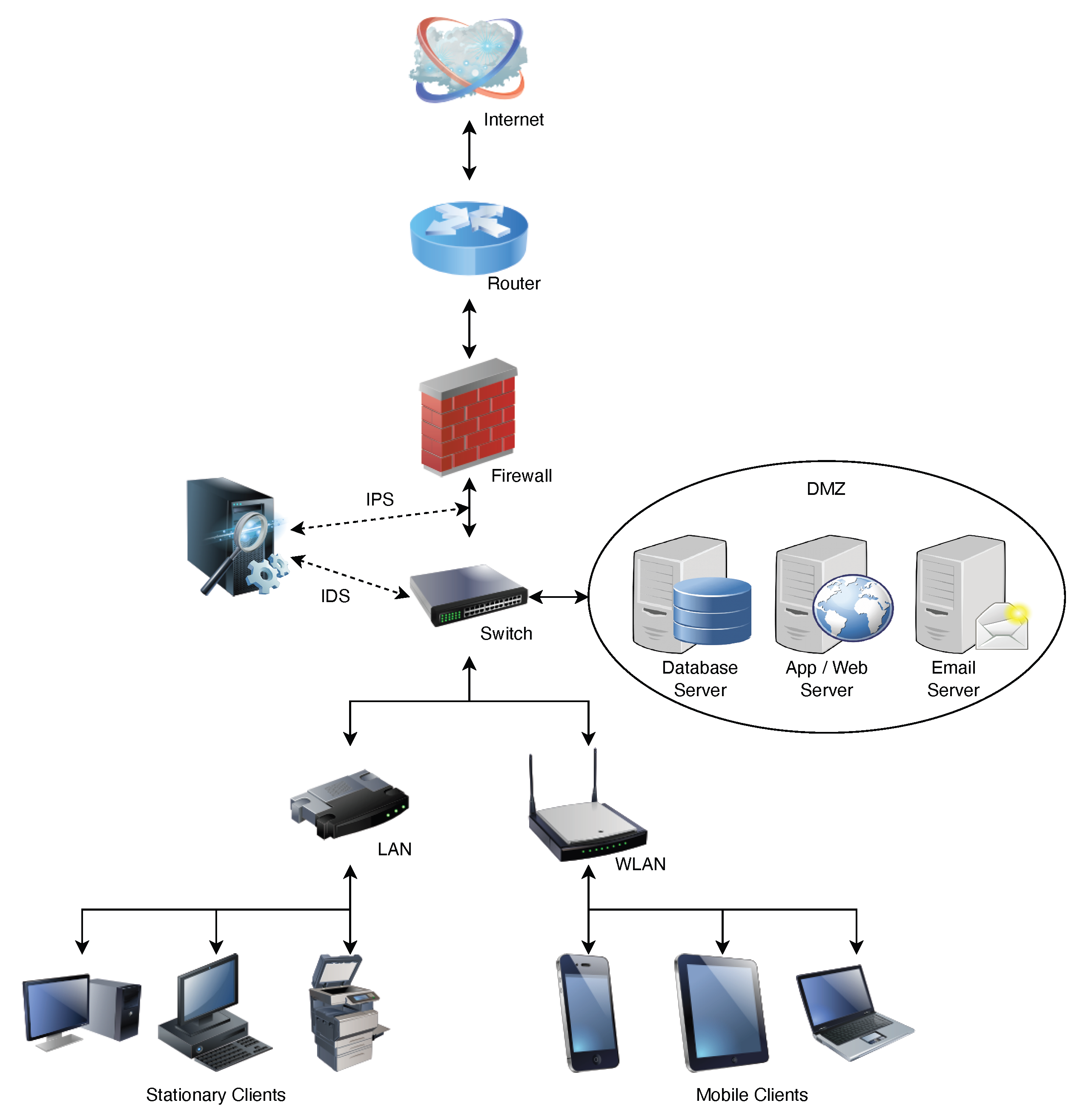
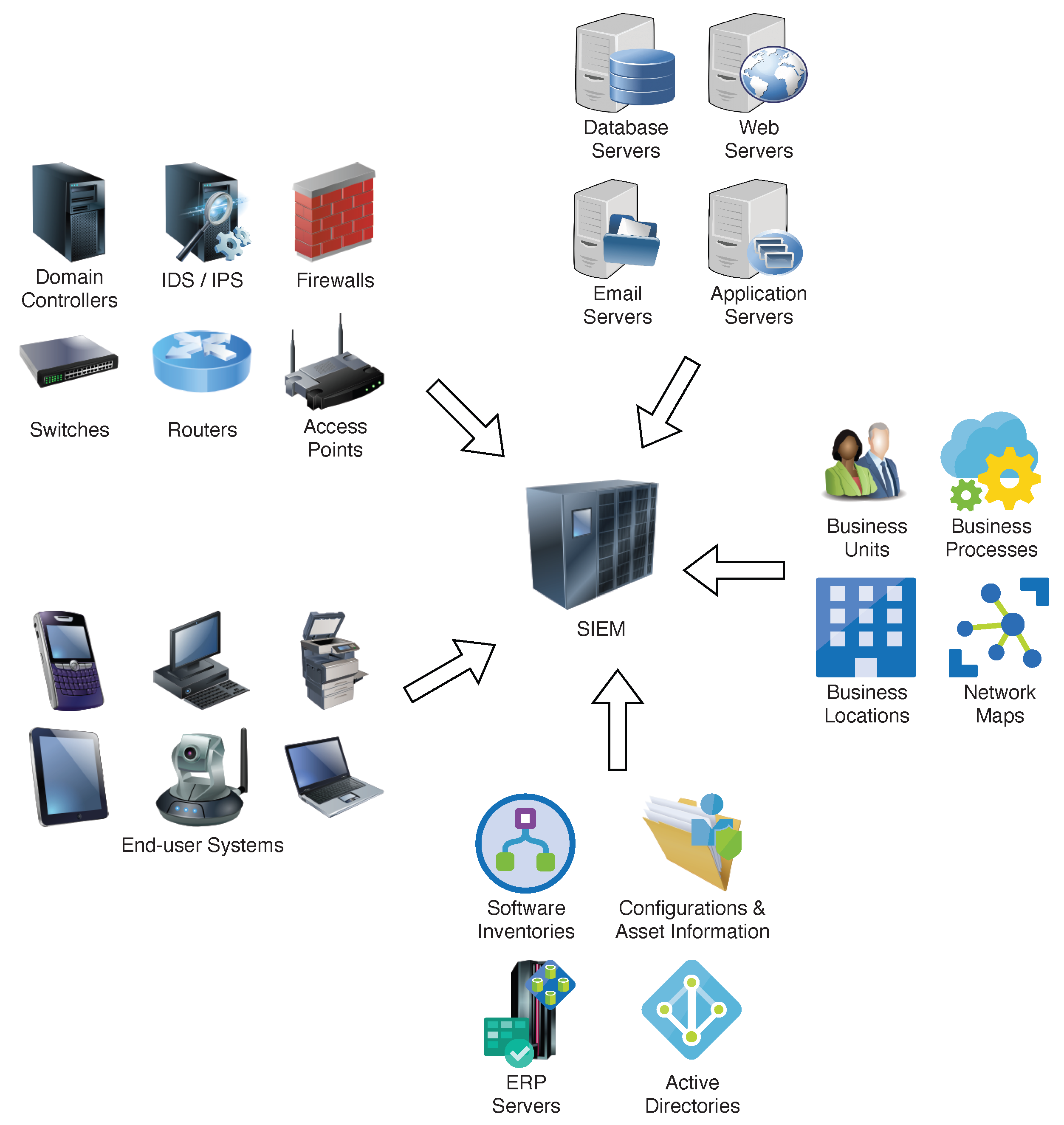
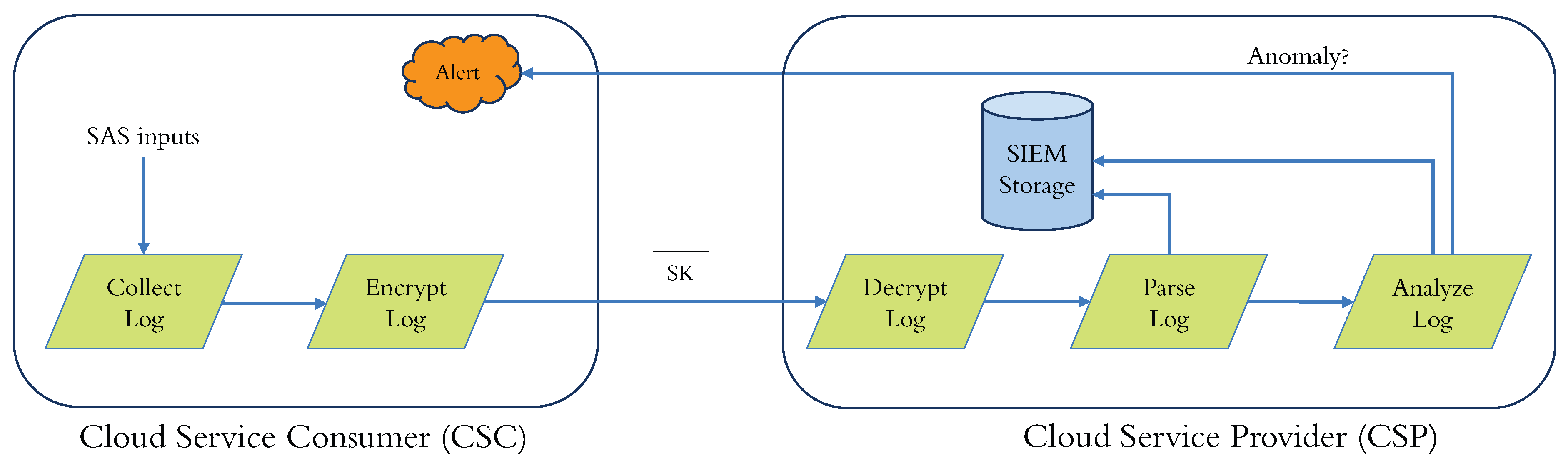
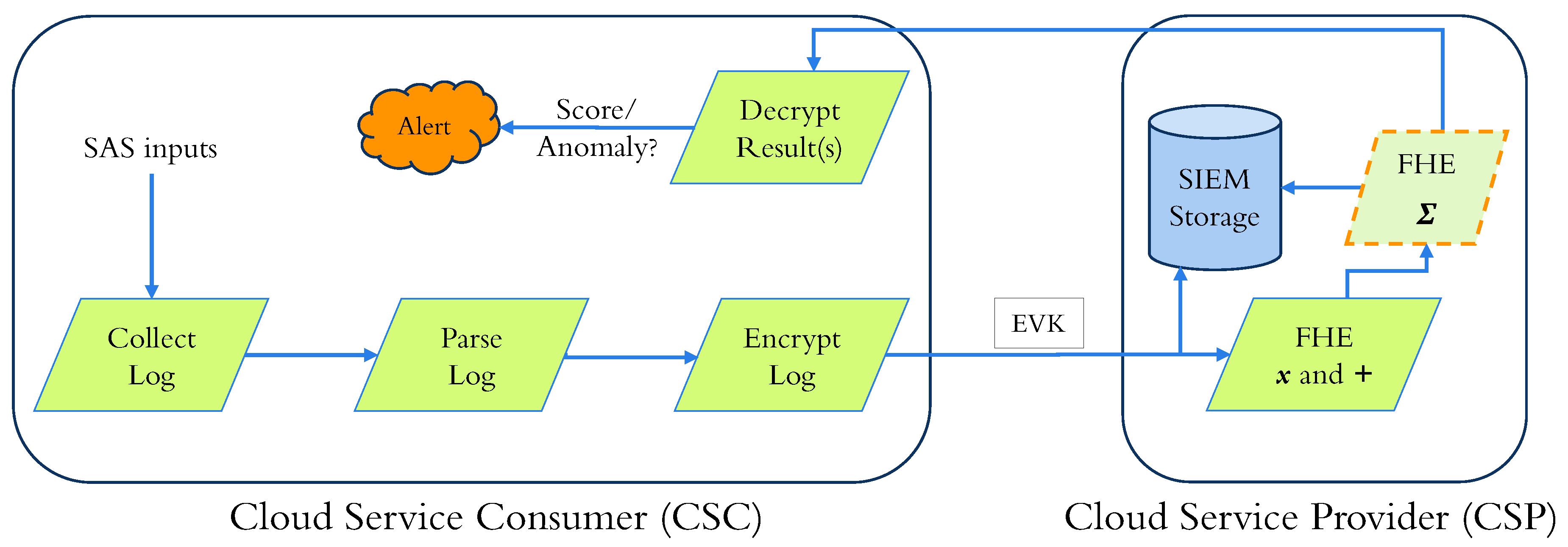
A “log collector” to collect logs from diverse applications operating on a SAS.

2.

A “transmitter” that sends logs to the SIEM, which is usually encrypted to safeguard against eavesdropping in the communication channel.

3.

A “receiver” to amass, store, decrypt, and ascertain the transmitted logs’ integrity.

4.

A “parser” to convert the data into a structured form used by the SIEM vendor to process the decrypted logs for storage and analysis.

5.

An “anomaly detector” that uses proprietary algorithms to render parsed logs and transmit alerts for anomalies.

SOCs use a variety of storage options for their SIEM databases, depending on their specific needs and requirements, including (i) servers located on-premises, (ii) Storage Area Network (SAN) or Network-Attached Storage (NAS), and (iii) cloud-based storage services, such as Amazon S3 [1] or Azure Blob Storage [2].

In a SOC, the relative jitter for the Log Collector (LC), Transmitter (TX), Receiver (RX), Parser (PA), and Anomaly Detector (AD) is the variation in the time it takes for each component to process a log event. Various factors, such as network latency, hardware performance, and software complexity, can cause this jitter. The AD has the highest relative jitter, followed by the PA, RX, TX, and LC. The AD is the most complex component, requiring more time to analyze each log event. The relative jitter of each component can significantly impact the overall performance of the SOC. For example, if the AD has a high relative jitter, detecting anomalies in the log data may take longer. This can lead to increased security risks. The relative jitter of each component can be reduced by (i) using high-performance hardware, (ii) optimizing the software, (iii) reducing network latency, and (iv) using load-balancing techniques in a SOC to improve overall performance and reduce security risks.

Enterprises frequently employ a third-party cloud vendor for the SOC. Third-party cloud services lessen the complexity and deliver flexibility for organizations. Nonetheless, Cloud Service Consumers (CSCs) must commission their data—and their customers’ data—to Cloud Service Providers (CSPs), who are often incentivized to monetize these data. Meanwhile, ordinances such as the US Consumer Online Privacy Rights Act (COPRA) [3], the US State of California Consumer Privacy Act (CCPA) [4], and the EU General Data Protection Regulation (GDPR) [5] strive to safeguard consumers’ privacy. Non-compliant institutions are subjected to stringent fines and deteriorated reputations. This outcome is a trade-off between data utility and privacy.

Exporting log data to an SIEM deployed on a third-party CSP is perilous, as the CSP requires access to plaintext (unencrypted) log data for alert generation. Moreover, the CSP may have adequate incentives to accumulate user data. These data are stored in the CSP’s servers and thus encounter diverse privacy and security threats like data leakage and the misuse of information [6,7,8,9,10,11]. Thus, shielding these logs’ privacy and confidentiality is crucial. We present Fully Homomorphic Encryption (FHE) to permit CSCs to ensure privacy without sabotaging their ability to attain insights from their data.

Traditional cloud storage and computation approaches using contemporaneous cryptography mandate that customer data be decrypted before operating on them. Thus, security policies are deployed to avert unauthorized admission to decrypted data. CSCs must entrust the Access Control Policies (ACPs) incorporated by their CSPs for data privacy (Figure 4). With FHE, data privacy is accomplished by the CSC via cryptography, leveraging rigid mathematical proofs. Consequently, the CSP will not be admitted to unencrypted customer data for computation and storage without a valid Secret Key (SK).

FHE allows calculations to be performed on encrypted data without decrypting them first. The results of these computations are stored in an encrypted form. Still, when decrypted, they are equivalent to the results that would have been obtained if the computations had been performed on the unencrypted data. Plaintexts are unencrypted data, while ciphertexts are encrypted data. FHE can enable privacy-preserving storage and computation and process encrypted data in commercial cloud environments. It is a promising technology with a wide range of potential applications.

For privacy-preserving log anomaly detection, one can use a hardware-based solution (e.g., a Trusted Execution Environment (TEE)) or a software-based approach (e.g., FHE). SGX-Log [12] and Custos [13] achieved private log anomaly detection using a TEE with Intel SGX. However, TEEs have limitations as to how much data can be stored. For example, Intel SGX has a limit of 128 MB. Hence, bit-wise FHE schemes like TFHE [14] or word-wise FHE schemes like BFV [15,16] and CKKS [17] are better for more significant amounts of data. Concrete-ML from Zama [18] used TFHE, which is efficient for smaller-scale arithmetic. Still, it is inefficient for more significant arithmetic operations (while amortized performance in CKKS can be improved with batching). For word-wise FHE schemes, one can employ BFV for integers and CKKS for approximate arithmetic. Hence, for Machine Learning (ML) tasks, CKKS is a better choice. Aymen et al. [19] used BFV for SVMs with a linear kernel. They experimentally calculated the best scaling factor value to convert floats to integers for better accuracy, which is not required in CKKS. SigML [20] used CKKS for LR and SVM.

1.1. Contributions

Our contributions can be summarized as follows:

• First, we formulate a supervised binary classification problem for log anomaly detection and implement it with the CKKS cryptosystem (in Section 4).
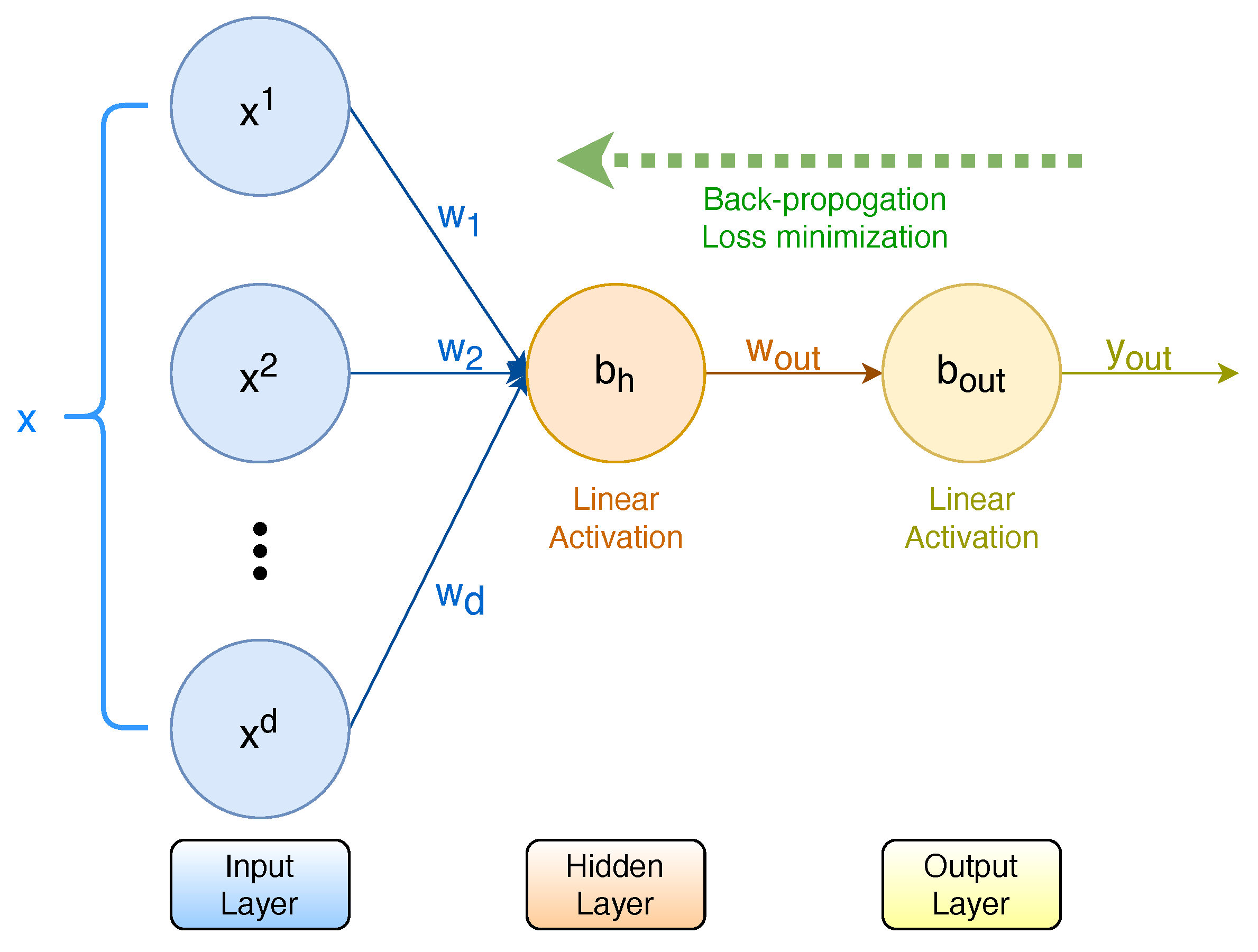
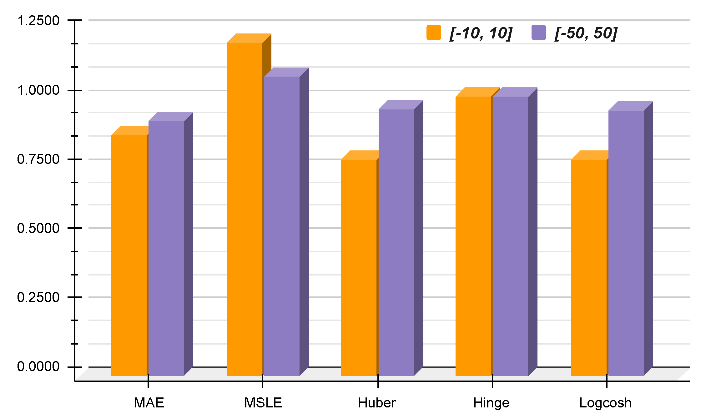
• Second, we propose novel ANN-based third-degree sigmoid approximations in the intervals $[-10,10]$ and $[-50,50]$ (in Section 5).
• Third, we evaluated the performance of various sigmoid approximations in the encrypted domain, and our results showed better accuracy and $\mathrm{\Sigma }$-ratio (in Section 6).

1.2. Organization

This paper is organized as follows:

• First, we describe the building blocks of our protocols in Section 2, where we review FHE in Section 2.1 and present polynomial approximations for the sigmoid $\left(\sigma \right(x\left)\right)$ activation function in Section 5.
• Next, we review the previous work in Section 3.
• Then, we describe our methodology in Section 4.
• Finally, we discuss our experimental results in Section 6.

2. Background

This section details CKKS, a fully homomorphic encryption scheme, and deterministic and probabilistic polynomial approximation schemes.

2.1. Fully Homomorphic Encryption

This work utilizes the CKKS [17] scheme as a fully homomorphic encryption scheme. CKKS varies from other FHE schemes (such as BFV [15,16], BGV [21], and TFHE [14]) in the way in which it interprets encryption noise. Indeed, CKKS treats encryption noise as part of the message, similar to how floating-point arithmetic approximates real numbers. This means the encryption noise does not eliminate the Most Significant Bits (MSBs) of the plaintext m as long as it stays small enough. CKKS decrypts the encryption of message m as an approximated value $m+e$, where e is a slight noise. The authors of CKKS suggested multiplying plaintexts by a scaling factor $\mathrm{\Delta }$ prior to encryption to lessen precision loss after adding noise during encryption. CKKS also sustains batching, a process for encoding many plaintexts within a single ciphertext in a Single Instruction Multiple Data (SIMD) fashion. We describe CKKS as a set of probabilistic polynomial-time algorithms regarding the security parameter $\lambda$.

The algorithms are:

• $\mathsf{CKKS}.\mathsf{Keygen}$—generates a key pair.
• $\mathsf{CKKS}.\mathsf{Enc}$—encrypts a plaintext.
• $\mathsf{CKKS}.\mathsf{Dec}$—decrypts a ciphertext.
• $\mathsf{CKKS}.\mathsf{Eval}$—evaluates an arithmetic operation on ciphertexts.

The level of a ciphertext is l if it is sampled from ${\mathbb{Z}}_{q_l}\left[X\right]/(X^N+1)$. Let $L,q_0$ and $\mathrm{\Delta }$ be integers. We set $q_l={\mathrm{\Delta }}^l·q_0$ for any l integer in $〚0,L〛$.

• $(evk,pk,sk)\leftarrow \mathsf{CKKS}.\mathsf{Keygen}(1^{\lambda },L)$: generates a secret key ($sk$) for decryption, a public key ($pk$) for encryption, and a publicly available evaluation key ($evk$). The secret key ($sk$) is a sample from a random distribution over ${\mathbb{Z}}_3\left[X\right]/(X^N+1)$. The public key ($pk$) is computed as

  $$pk=({[-a·sk+e]}_{q_L},a)=(p_0,p_1)$$

  where a is sampled from a uniform distribution over ${\mathbb{Z}}_{q_L}\left[X\right]/(X^N+1)$, and e is sampled from an error distribution over ${\mathbb{Z}}_{q_L}\left[X\right]/(X^N+1)$. $evk$ is utilized for relinearization after the multiplication of two ciphertexts.
• $c\leftarrow \mathsf{CKKS}.{\mathsf{Enc}}_{pk}\left(m\right)$: encrypts a message m into a ciphertext c utilizing the public key ($pk$). Let v be sampled from a distribution over ${\mathbb{Z}}_3\left[X\right]/(X^N+1)$. Let $e_0$ and $e_1$ be small errors. Then, the message m is encrypted as

  $$c={[(v·p{k}_0,v·p{k}_1)+(m+e_0,e_1)]}_{qL}=(c_0,c_1).$$
• $m\leftarrow \mathsf{CKKS}.{\mathsf{Dec}}_{sk}\left(c\right)$: decrypts a message c into a plaintext m utilizing the secret key ($sk$). The message m can be recovered from a level l ciphertext thanks to the function $m={[c_0+c_1·sk]}_{q_l}$. Note that with CKKS, the capacity of a ciphertext reduces each time a multiplication is computed.
• $c^{\left(f\right)}\leftarrow \mathsf{CKKS}.{\mathsf{Eval}}_{evk}(f,c^{\left(1\right)},c^{\left(2\right)},\cdots ,c^{\left(k\right)})$: estimates the function f on the encrypted inputs $(c^{\left(1\right)},c^{\left(2\right)},\cdots ,c^{\left(k\right)})$ using the evaluation key $\mathsf{evk}$.

2.2. Polynomial Approximations

This section describes commonly used (deterministic) function interpolation techniques like the (i) Taylor, (ii) Fourier, (iii) Pade, (iv) Chebyshev, (v) Remez, and our (vi) probabilistic ANN scheme.

2.2.1. Taylor

The Taylor series (Equation (1)) is a mathematical expression approximating a function as an infinite sum of terms expressed in terms of the function’s derivatives at a single point a, called the center of the Taylor series. The Maclaurin series is a particular case of the Taylor series where the center of the series is $a=0$. In other words, a Maclaurin series is a Taylor series centered at zero. It is a power series that permits the calculation of an approximation of a function $f\left(x\right)$ for input values near zero, given that the values of the successive derivatives of the function at zero are known. The Maclaurin series can be used to find the antiderivative of a complicated function, approximate a function, or compute an incomputable sum. In addition, the partial sums of a Maclaurin series provide polynomial approximations for the function.

$$\sum _{n=0}^{\infty }{f}^{\left(n\right)}\left(a\right)\frac{{(x-a)}^n}{n!}=f\left(a\right)+f^{\prime }\left(a\right)(x-a)+\frac{f^{\prime \prime }\left(a\right)}{2!}{(x-a)}^2+\dots +\frac{f^{\left(k\right)}\left(a\right)}{k!}{(x-a)}^n+\dots$$

(1)

2.2.2. Fourier

The Fourier series can be represented in sine-cosine, exponential, and amplitude-phase forms. For a sine-cosine form, the coefficients are

$$\begin{array}{cc}\hfill & A_0=\frac{1}{P}{\int }_{-P/2}^{P/2}f\left(x\right)dx\hfill \\ & A_n=\frac{2}{P}{\int }_{-P/2}^{P/2}f\left(x\right)cos\left(\frac{2\pi nx}{P}\right)dx\hfill \\ \hfill & B_n=\frac{2}{P}{\int }_{-P/2}^{P/2}f\left(x\right)sin\left(\frac{2\pi nx}{P}\right)dx\hfill \end{array}$$

(2)

With these coefficients, the Fourier series is

$$f\left(x\right)\sim A_0+\sum _{n=1}^{\infty }{A}_{n}cos\left(\frac{2\pi nx}{P}\right)+B_{n}sin\left(\frac{2\pi nx}{P}\right)$$

(3)

For an exponential form, the coefficients are

$$\begin{array}{cc}\hfill & c_0=A_0\hfill \\ & c_n=(A_n-i{B}_n)/2,\mathrm{for}n>0\hfill \\ \hfill & c_n=(A_{-n}+i{B}_{-n})/2,\mathrm{for}n<0\hfill \end{array}$$

(4)

By substituting Equation (2) into Equation (4),

$$c_n=\frac{1}{P}{\int }_{-P/2}^{P/2}f\left(x\right)e^{-\frac{2\pi inx}{P}}dx$$

(5)

With these definitions, we can write the Fourier series in exponential form:

$$f\left(x\right)=\sum _{n=-\infty }^{\infty }{c}_n·e^{\frac{2\pi inx}{P}}$$

(6)

2.2.3. Pade

Given a function f and two integers $m\ge 0$ and $n\ge 1$, the Pade approximant of order $[m/n]$ is the rational function

$$R\left(x\right)=\frac{{\mathrm{\Sigma }}_{j=0}^m{a}_j{x}^j}{1+{\mathrm{\Sigma }}_{k=1}^n{b}_k{x}^k}=\frac{a_0+a_{1}x+a_2{x}^2+\dots +a_m{x}^m}{1+b_{1}x+b_2{x}^2+\dots +b_n{x}^n},$$

(7)

which agrees with $f\left(x\right)$ to the highest possible order, amounting to

$$\begin{array}{cc}\hfill & f\left(0\right)=R\left(0\right),\hfill \\ \hfill & f^{\prime }\left(0\right)=R^{\prime }\left(0\right),\hfill \\ & f^{\prime \prime }\left(0\right)=R^{\prime \prime }\left(0\right),\hfill \\ \hfill & ⋮\hfill \\ \hfill & f^{(m+n)}\left(0\right)=R^{(m+n)}\left(0\right)\hfill \end{array}$$

(8)

Equivalently, if $R\left(x\right)$ is expanded in a Taylor series at 0, its first $m+n$ terms would cancel the first $m+n$ terms of $f\left(x\right)$, and as such

$$f\left(x\right)-R\left(x\right)=c_{m+n+1}{x}^{m+n+1}+c_{m+n+2}{x}^{m+n+2}+\dots$$

(9)

2.2.4. Chebyshev

The Chebyshev polynomial of degree n is denoted $T_n\left(x\right)$ and is given by the formula

$$T_n\left(x\right)=cos(narccosx)$$

(10)

The first few Chebyshev polynomials of this kind are

$$\begin{array}{cc}\hfill & T_0\left(x\right)=1\hfill \\ \hfill & T_1\left(x\right)=x\hfill \\ & T_2\left(x\right)=2x^2-1\hfill \\ \hfill & \cdots \hfill \\ \hfill & T_{n+1}\left(x\right)=2x{T}_n\left(x\right)-T_{n-1}\left(x\right)\hfill \end{array}$$

(11)

If $f\left(x\right)$ is an arbitrary function in the interval $[-1,1]$, and if N coefficients $c_j$, $j=0,\dots ,N-1$, are defined by

$$c_j=\frac{2}{N}\sum _{k=1}^{N}f\left(x_k\right)T_j\left(x_k\right)=\frac{2}{N}\sum _{k=1}^{N}f\left. [cos\left(\frac{\pi (k-\frac{1}{2})}{N}\right)\right]cos\left(\frac{\pi j(k-\frac{1}{2})}{N}\right),$$

(12)

then, we obtain the approximation formula

$$f\left(x\right)\approx \left. [\sum _{k=0}^{N-1}{c}_k{T}_k\left(x\right)\right]-\frac{1}{2}{c}_o$$

(13)

2.2.5. Remez

Given a function, $f\left(x\right)$ to be approximated and a set X of $n+2$ points $x_1,x_2,\dots ,x_{n+2}$ in the approximation interval, the extrema of the Chebyshev polynomial are usually linearly mapped to the interval. The Remez algorithm is the following:

1.

Solve the system of linear equations

$$b_0+b_1{x}_i+\dots +b_n{x}_i^n+{(-1)}^{i}E=f\left(x_i\right);i=1,2,\dots ,n+2$$

(14)

for the unknowns $b_0,b_1,\dots ,b_n$ and E.

2.

Use $b_i$ as coefficients to form a polynomial $P_n$.

3.

Find the set M of points of local maximum error $|P_n\left(x\right)-f\left(x\right)|$.

4.

If the errors at every $m\in M$ are alternate in sign (+/−) and of equal magnitude, then $P_n$ is the minimax approximation polynomial. If not, replace X with M and repeat the abovementioned steps.

2.2.6. ANN

While Artificial Neural Networks (ANNs) are known for their universal function approximation properties, they are often treated as black boxes and used to calculate the output value. We propose the use of a basic three-layer Perceptron (Figure 5) consisting of an input layer, a hidden layer, and an output layer, with both hidden and output layers having linear activations to generate the coefficients for an approximation polynomial of a given order. In this architecture, the input layer is dynamic, with the input nodes corresponding to the desired polynomial degrees. While having a variable number of hidden layers is possible, we fix it at a single layer with a single node to minimize the computation. We show coefficient calculations for a third-order polynomial ($d=3$); a univariate function $f\left(x\right)=y$; and an input x, actual output y, and predicted output $y_{out}$. The input layer weights are

$$\{w_1,w_2,\dots ,w_d\}=\{w_1,w_2,w_3\}=\{x,x^2,x^3\}$$

, and the biases are $\{b_1,b_2,b_3\}=b_h$. Thus, the output of the hidden layer is

$$y_h=w_{1}x+w_2{x}^2+w_3{x}^3+b_h$$

The predicted output is calculated by

$$y_{out}=w_{out}·y_h+b_{out}=w_1{w}_{out}x+w_2{w}_{out}{x}^2+w_3{w}_{out}{x}^3+(b_h{w}_{out}+b_{out})$$

(15)

Where the layer weights $\{w_1{w}_{out},w_2{w}_{out},w_3{w}_{out}\}$ are the coefficients for the approximating polynomial of order three and the constant term is $b_h{w}_{out}+b_{out}$.

Since the predicted output ($y_{out}$) is probabilistic, it must be fine-tuned with hyperparameter tuning, as incorrect results lead to erroneous (inefficient) approximations.

Trivedi [22] provided third and seventh-degree polynomial approximations for univariate $Sign\left(x\right)\in \{-1,0,1\}$ and $Compare(a-b)\in \{0,\frac{1}{2},1\}$ functions in the intervals $[-1,1]$ and $[-5,-5]$. Trivedi [22] empirically showed that their novel ANN polynomials improved up to 15% accuracy (regarding losses) over Chebyshev’s.

3. Related Work

This section discusses previous research on privacy-preserving log management architectures. Zhao et al. [23] proposed a system called Zoo to minimize latency in data processing and reduce the amount of raw data exposed to the Cloud Service Provider (CSP). Zoo is deployed on Customer-owned Edge Devices (CEDs) rather than on the cloud, and it supports the composition, construction, and easy deployment of Machine Learning (ML) models on CEDs and local devices. Zoo is implemented in the OCaml language on top of the open-source numerical computing system Owl [24]. In addition to CEDs, Zoo can be deployed on cloud servers or a hybrid of both. This can further reduce the data exposed to the CSP and its communication costs. Repositioning ML-based data analytics to edge devices from the cloud poses hurdles such as resource limitations, a scarcity of usable models, and difficulty deploying user services. Additionally, deploying services on a CED environment introduces problems for the CSP, as the privacy of ML models (weights) must be shielded from the CED.

Ray et al. [25] proposed a set of protocols for the anonymous uploading, retrieving, and deleting of log records in the cloud using the Tor [26] network. Their scheme addresses integrity and security issues throughout the log management, including log collection, transmission, retrieval, and storage. However, their logging client is operating-system-specific, and privacy is not guaranteed because logs can be identified by their tag values.

Zawoad et al. [27,28] presented Secure Logging as a Service (SecLaaS), which stores and provides access to logs generated by Virtual Machines (VMs) running in the cloud. SecLaaS ensures the confidentiality and integrity of these logs, which the CSCs own. SecLaaS encrypts some Log Entry (LE) information utilizing a public key shared by the security agents to ensure confidentiality. The private key to decrypt the log is shared among the security agents. An auditor can verify the integrity of the logs utilizing the Proof of Past Log (PPL) and the Log Chain (LC). However, SecLaaS cannot encrypt all the fields of the LE, as the CSP needs to be able to search the storage by some fields. Additionally, using a shared public key violates the CSC’s data privacy.

Rane and Dixit [29] presented BlockSLaaS, a blockchain-assisted Secure Logging-as-a-Service system for cloud environments. BlockSLaaS aims to make the cloud more auditable and forensic-friendly by securely storing and processing logs while tackling multi-stakeholder collusion problems and ensuring integrity and confidentiality. The integrity of logs is assured by utilizing the immutable property of blockchain technology. Cloud Forensic Investigators (CFIs) can only access the logs for forensic investigation through BlockSLaaS, which preserves the confidentiality of logs. To ensure the privacy of the CSC, the Node Controller (NC) encrypts each log entry utilizing the CFI’s public key, $CF{I}_{PK}$. The CFI can then utilize its secret key, $CF{I}_{SK}$, to decrypt the logs, preserving the confidentiality of the CSC’s logs. However, this scheme utilizes the CFI’s public key, which violates the data privacy of the CSC. A more effective privacy-preserving scheme would use a different keying mechanism, such as a private blockchain or a Trusted Execution Environment (TEE).

Bittau et al. [30] presented a principled systems architecture called Encode, Shuffle, Analyze (ESA) for performing large-scale monitoring with high utility while safeguarding user privacy. ESA guarantees the privacy of monitored users’ data by processing it in a three-step pipeline:

1.

Encode: The data are encoded to control their scope, granularity, and randomness.

2.

Shuffle: The encoded data are shuffled to break their linkability and guarantee that individual data items become “lost in the crowd” of the batch.

3.

Analyze: The anonymous, shuffled data are analyzed by a specific analysis engine that averts statistical inference attacks on analysis results.

The authors implemented ESA as a system called PROCHLO, which develops new techniques to harden the three steps of the pipeline. For example, PROCHLO uses Stash Shuffle, a novel, efficient, and scalable oblivious-shuffling algorithm based on Intel’s SGX, a TEE. TEEs provide isolated execution environments where code and data can be protected from the host system. However, using a TEE like Intel SGX may only be practical for some devices and infeasible for legacy and low-resourced systems. Additionally, TEEs limit the amount of data that can be secured.

Paul et al. [31] presented a secure collective learning protocol for sharing classified time-series data within entities to partially train the parameters of a binary classifier model. They approximated the sigmoid activation function ($\sigma \left(x\right)$) to a polynomial of degree seven. They presented a collective learning protocol to apply Homomorphic Encryption (HE) to fine-tune the last layer of a Deep Neural Network (DNN) securely. However, degree-seven approximation using an HE method is counterproductive for resource-constrained machines, such as wireless sensors or Internet-of-Things (IoT) devices.

The work most comparable to ours on log confidentiality during transmission and analysis using FHE techniques was presented by Boudguiga et al. [19]. In their scheme, the authors examined the feasibility of using FHE to furnish a privacy-preserving log management architecture. They utilized Support Vector Machines (SVMs) with a linear kernel to assess the FHE classification of Intrusion Detection System (IDS) alerts from the NSL-KDD dataset. In their scheme, they encrypted the input data from an SAS using the BFV scheme and performed FHE calculations on the encrypted data using the SIEM weights in plaintext. The encrypted results for each log entry were then sent back to the SAS for decryption. However, this approach could be vulnerable to inference attacks by malicious SAS, such as attribute inference, membership inference, and model inversion attacks. Our “Aggregate” scheme helps prevent most of these attacks, as it only sends a total anomaly score (sum) per block instead of predictions or labels per input, thus minimizing the data inferred by the attacker.

SigML, proposed by Trivedi et al. [20], uses the CKKS scheme and presents:

1.

Ubiquitous configuration—This is similar to other works and sends an encrypted result for every log entry.

2.

Aggregate configuration—This reduces communication and computation requirements by sending a single result for a block of log entries.

SigML compares three approximations of the sigmoid function: ${\sigma }^1\left(x\right),{\sigma }^3\left(x\right)$, and ${\sigma }^5\left(x\right)$. These approximations are used for a Logistic Regression (LR) and Support Vector Machine (SVM) model. The authors observed that the LR and SVM models trained from scikit-learn [32] did not perform well with the sigmoid activation for the “Aggregate” configuration. Therefore, they designed Sigmoid-LR (${\sigma }_{LR}$) to improve performance. Sigmoid-LR uses a kernel $A=X·W+b$ to reduce the errors of $sigmoid\left(a\right)$ with the learning rate $r_{learn}$ and the number of iterations $r_{iter}$. The inputs and labels are $X,Y\in [0,1]$. This paper presents “SigML++”, an extension of SigML [20]. SigML++ improves the results of SigML with LR and SVM models using a novel ANN approximation. SigML++ also evaluates third-order polynomials in the intervals $[-10,10]$ and $[-50,50]$.

4. Proposed Solution

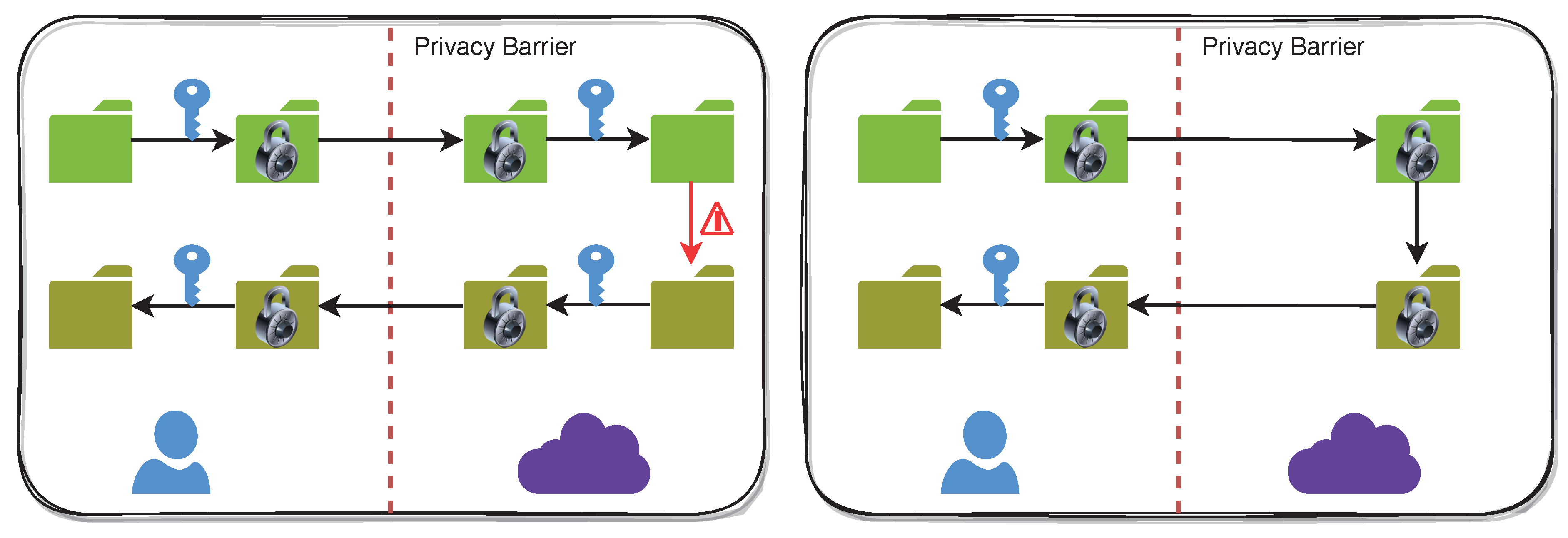
Our threat model considers an SAS (CSC) and an SIEM (CSP) for simplicity. The SAS is the client that wants to generate anomaly alerts from logs while preserving its privacy. Consequently, the SIEM server should be oblivious to the data received and refrain from comprehending the log information. On the other hand, the SIEM also desires to shield the weights and coefficients of the ML model used to detect intrusion anomalies and generate alerts. Thus, the SAS should refrain from learning about the model information.

For log analysis using FHE, log parsing shifts from the SIEM to the SAS. Instead of the SIEM decrypting and parsing the logs, the SAS collects and parses unstructured logs to a structured form and normalizes the data. Data normalization helps to enhance ML model prediction. The SAS uses FHE to generate an encryption key ($pk/sk$), a decryption key ($sk$), and an evaluation key ($evk$). The parsed log inputs are encrypted using the public key ($pk$) or secret key ($sk$). We use the CKKS scheme for FHE, better suited for floating-point value calculations. CKKS is more suited for arithmetic on real numbers, where one can obtain approximate but close results, while BFV is more suited for arithmetic on integers. The SIEM performs homomorphic computations on the encrypted inputs and the ML model’s coefficients in plaintext, using the evaluation key ($evk$) generated by the SAS. The encrypted results are then passed to the SAS. The SAS decrypts the results with the secret key ($sk$), infers whether there was an anomaly, and generates an alert accordingly.

We present (i) “Ubiquitous” and (ii) “Aggregate” configurations similar to SigML. While the “Ubiquitous” configuration is similar to prevalent research works, the “Aggregate” configuration reduces the computation and communication requirements of the SAS.

The configurations differ in how SIEM results are generated and processed at the SAS:

1.

Ubiquitous—The SIEM sends one encrypted result per user input.

2.

Aggregate—Only one result is sent to the encrypted domain for all the user inputs. This technique helps reduce communication costs and uses much fewer resources on the SAS to decrypt a single encrypted result rather than one encrypted result per encrypted input.

In the “Ubiquitous” configuration (Figure 6), the SAS sends encrypted parsed inputs to the SIEM for analysis, and the SIEM performs homomorphic calculations on the encrypted inputs and unencrypted weights. The SIEM sends one encrypted result to the SAS for every encrypted log entry in the received block. The SAS decrypts all the results and evaluates the labels for all the individual log entries. In this configuration, the disadvantage is the data leakage used for training or the model weights, as a dishonest client can perform inference attacks.

In the “Aggregate” configuration (Figure 6), the SAS sends a block of encrypted parsed inputs as before. The SIEM performs homomorphic computation with plaintext model weights for each input in the received block, applies sigmoid approximation to individual encrypted results, and sums (via homomorphic additions) all encrypted results.

The sigmoid activation is a mathematical function that approximates the outputs of a machine learning model in the $[0,1]$ range. In log anomaly detection, a label 0 corresponds to a “normal” class, and a 1 corresponds to an “anomalous” class. In the proposed procedure, the SAS receives only one result per block of messages. This saves network bandwidth, as the SAS does not need to receive individual ciphers (encrypted labels) for each message. Additionally, the SAS only needs to decrypt one cipher (encrypted total) per block, which saves storage and computation overhead. The SAS decrypts the result and assesses the sum for the block of messages. If there are no abnormalities in the block, the totality should be 0. Otherwise, it should be the count of anomalous inputs.

Another advantage of this configuration is that it utilizes an anomaly score per block of log entries and functions as a litmus test for log anomalies. For example, a SOC engineer may prefer to examine the block of logs with a higher anomaly score than a block with a much lower score. Furthermore, if there are successive blocks with higher than usual anomaly scores, it may function as an IoC. The drawback of this configuration is that the SAS cannot pinpoint which entry in the block is anomalous.

As shown in

Table 1. Comparison of “Ubiquitous” and “Aggregate” configurations.

Configuration	Encryption		Decryption
	Time	Size	Time	Size
Ubiquitous Aggregate	$n·T_E\left(p\right)$	$n·S_E\left(p\right)$	$n·T_D\left(c\right)$ $T_D\left(c\right)$	$n·S_D\left(c\right)$ $S_D\left(c\right)$

, n is the number of logs, $T_E\left(p\right)$ is the time taken to encrypt a single message, $S_E\left(p\right)$ is the bytes occupied by a single ciphertext, $T_D\left(c\right)$ is the time taken to decrypt a single ciphertext, and $S_D\left(c\right)$ is the bytes occupied by a single (decrypted) message. We first trained the ML models using LR and SVM in plaintext and performed inference on encrypted data, as the inputs to the model are encrypted. The calculations were performed on plaintext weights of the model, yielding the encrypted results. This also helped to create a baseline to compare the performance of various approximations in encrypted domains.

5. Sigmoid Approximation

Barring message expansion and noise growth, applying the sigmoid activation function is a substantial challenge in implementing ML with FHE. The sigmoid function is used in LR and SVMs during classification, so we determined to make it homomorphic. We further describe techniques to approximate this activation function with a polynomial for word-wise FHE and compare various polynomial approximations in terms of accuracy, precision, recall, F1-score, and the $\mathrm{\Sigma }$-ratio of the predicted sum from sigmoid values to the sum of all actual binary labels for the test dataset. We denote ${\mathbf{M}}_{\mathbf{i}}^{\mathbf{d}}$, where $\mathbf{M}$ is an approximation method like Taylor ($\mathbf{T}$), Remez ($\mathbf{R}$), Chebyshev ($\mathbf{C}$), or ANN ($\mathbf{A}$); $\mathbf{d}$ is the degree; and $\mathbf{i}$ is the interval $[-\mathbf{i},\mathbf{i}]$ of the polynomial. We approximate the class $C[a,b]$ of continuous functions on the interval $[a,b]$ by order-n polynomials in ${\mathcal{P}}_n$ using the $L^{\infty }$-norm to measure the fit. This is called minimax polynomial approximation since the best (or minimax) approximation solves

$$p_n^{*}=arg\underset{p_n\in {\mathcal{P}}_n}{min}\underset{a\le x\le b}{max}|f\left(x\right)-p_n\left(x\right)|$$

(16)

A minimax approximation is a technique to discover the polynomial p in Equation (16), i.e., the Remez algorithm [33] is an iterative minimax approximation and outputs the following results [34] for the interval [−5, 5] and order three:

$${\mathbf{R}}_{\mathbf{5}}^{\mathbf{3}}\left(\mathbf{x}\right)=0.5+0.197x-0.004x^3$$

(17)

The Taylor series (around point 0) of degree three is given by

$${\mathbf{T}}^{\mathbf{3}}\left(\mathbf{x}\right)=0.5+0.25x-0.0208333x^3$$

(18)

The Chebyshev series of degree three for the interval $[-10,10]$ is

$$0.5+0.139787x+(3.03084e-26)x^2-0.00100377x^3$$

We omit the term for $x^2$ to obtain

$${\mathbf{C}}_{\mathbf{10}}^{\mathbf{3}}\left(\mathbf{x}\right)=0.5+0.139787x-0.00100377x^3$$

(19)

Similarly, we obtain the Chebyshev series of degree three for the interval $[-50,50]$

$${\mathbf{C}}_{\mathbf{50}}^{\mathbf{3}}\left(\mathbf{x}\right)=0.5+0.0293015x-(8.65914e-6)x^3$$

(20)

We derive the ANN polynomials of degree three for $[-10,10]$

$${\mathbf{A}}_{\mathbf{10}}^{\mathbf{3}}\left(\mathbf{x}\right)=0.49961343+0.12675145x-0.00087002286x^3$$

(21)

and for the interval $[-50,50]$

$${\mathbf{A}}_{\mathbf{50}}^{\mathbf{3}}\left(\mathbf{x}\right)=0.49714848+0.026882438x-(7.728304e-06)x^3$$

(22)

We compared the Chebyshev and ANN approximations for the sigmoid functions as shown in

Table 2. Polynomial approximation losses for the intervals $[-10,10]$ and $[-50,50]$.

Interval	Method	MAE	MSLE	Huber	Hinge	Logcosh
$[-10,10]$	${\mathbf{C}}_{\mathbf{10}}^{\mathbf{3}}$	0.0793	0.0020	0.0039	0.5593	0.0039
	${\mathbf{A}}_{\mathbf{10}}^{\mathbf{3}}$	0.0691	0.0024	0.0031	0.5646	0.0031
$[-50,50]$	${\mathbf{C}}_{\mathbf{50}}^{\mathbf{3}}$	0.1363	0.0115	0.0138	0.5475	0.0136
	${\mathbf{A}}_{\mathbf{50}}^{\mathbf{3}}$	0.1255	0.0124	0.0132	0.5534	0.0131

. We calculated the mean absolute error (MAE); mean squared log error (MSLE); and Huber, Hinge, and Logcosh losses [35,36] for the Chebyshev polynomials described in Equations (19) and (20) and ANN polynomials from Equations (21) and (22), e.g., ${\mathbf{A}}_{\mathbf{10}}^{\mathbf{3}}$ recorded an MAE loss of $0.0691$ compared to $0.0793$ for ${\mathbf{C}}_{\mathbf{10}}^{\mathbf{3}}$.

The lower losses (closer to 0) reflect fewer errors, showing that a better approximation was achieved using our approach. Comparing their ratios $\frac{0.0691}{0.0793}=0.8712$, we observed a $\approx 14\%$ improvement (Figure 7).

6. Experimental Analysis

The experiments were conducted on a 2.4 GHz Quad-Core MacBook Pro with an Intel Core i5 processor and 2133 MHz 8 GB LPDDR3 memory. We used the SEAL-Python [37] library for Python3 to implement CKKS encryption. Moreover, we used sklearn [38] APIs for binary classifiers.

6.1. Evaluation Criteria

We compared the performance of the models using the following metrics: precision, recall, accuracy, and F1-score for the “Ubiquitous” configuration and $\mathrm{\Sigma }$-ratio for the “Aggregate” configuration. We repeated the experiments on both the NSL-KDD and the balanced HDFS datasets.

• Precision is the proportion of correctly predicted positive results (true positive, TP) to the total predicted positive results (TP + false positive, FP). It is also known as the positive predictive value.
• Recall is the proportion of correctly predicted positive results (TP) to the total actual positive results (TP + false negative, FN). It is also known as sensitivity or specificity.
• Accuracy is the proportion of all correct predictions (TP + TN) to the total number of predictions made (TP + FP + TN + FN). It can be calculated as precision divided by recall or $1-\frac{FalseNegativeRate\left(FNR\right)}{FalsePositiveRate\left(FPR\right)}$.
• The F1-score is a measure that considers both precision and recall. It is calculated as the harmonic mean of the precision and recall.
• The $\mathrm{\Sigma }$-ratio is measured for the sigmoid activation function with binary outcomes and calculated as the ratio of the sum of all predicted labels to the sum of all actual labels.

$$Precision=\frac{TP}{TP+FP}$$

(23)

$$Recall=\frac{TP}{TP+FN}$$

(24)

$$Accuracy=\frac{TP+TN}{TP+FP+TN+FN}$$

(25)

$$F1-Score=2\ast \frac{Precision\ast Recall}{Precision+Recall}$$

(26)

$$\mathrm{\Sigma }-Ratio=\frac{{\sum }_{i=1}^n\mathrm{Predicted}{y}_i}{{\sum }_{i=1}^n\mathrm{Actual}{y}_i},\mathrm{where}{y}_i\in \{0,1\}$$

(27)

6.2. Datasets

Log datasets are often imbalanced, with most samples belonging to one class. This can lead to overfitting and a “pseudo-high” accuracy for the trained model. To avoid this, we proposed the use of balanced datasets. We first used a “Return-1 Model” (

Table 3. Return-1 model performance for NSL-KDD and HDFS.

Dataset	Type	Accuracy	Precision	Recall	F1-Score	$\mathit{\Sigma }$-Ratio
NSL-KDD	Full (100%)	0.4811	0.4811	1.0000	0.6497	2.0782
	Test (20%)	0.4832	0.4832	1.0000	0.6515	2.0695
HDFS	Full (100%)	0.4999	0.4999	1.0000	0.6666	2.0000
	Test (20%)	0.5016	0.5016	1.0000	0.6681	1.9934

) to verify the balance of classes in our log anomaly datasets. This model always classifies samples as “anomalous”. We achieved an accuracy of 48.11% and a $\mathrm{\Sigma }$-ratio of 2.07 for the NSL-KDD dataset and an accuracy of 49.99% and $\mathrm{\Sigma }$-ratio of 2.00 for the HDFS dataset. We also achieved a recall of 100% for both datasets, as the model always outputs 1 for “anomaly”. The NSL-KDD [39] dataset is a modified version of the KDD’99 [40] dataset that solves some of the latter’s intrinsic problems. It contains 148,517 inputs with 41 features and two observations for score and label. We modified the labels to create a binary classification problem, with all attack categories consolidated into label 1. This resulted in 77,054 inputs with label 0 (“normal”) and 71,463 inputs classified as label 1 (“anomalous”). The testing set comprised 29,704 inputs, with 14,353 instances of label 1 and 15,351 of label 0. The HDFS_1 [41] labeled dataset from Logpai represents 1.47 GB of HDFS logs forged by running Hadoop-based map-reduce jobs on over 200 Amazon EC2 nodes for 38.7 h. Hadoop domain experts labeled this dataset. Of the 11,175,629 log entries accumulated, 288,250 (∼2.58%) are anomalous. We used Drain [42], a log parser, to convert our unstructured log data into a structured format. For brevity, we omit the textual log data parsing details here. We created a more undersized, balanced dataset of 576,500 inputs with seven observations equally distributed among the “normal” and “anomaly” classes. We used 20% of the total dataset as testing data, with 115,300 inputs, of which 57,838 inputs belonged to label 1 and 57,462 belonged to label 0.

6.3. Test Results

First, we constructed baselines with plain (unencrypted) data, and the results are exhibited in

Table 4. Comparison of performance metrics for sigmoid approximations.

Dataset	Model	Scale	Method	Accuracy	Precision	Recall	F1-Score	$\mathit{\Sigma }$-Ratio
NSL-KDD	LR		Plain	0.9352	0.9502	0.9138	0.9317	0.9966
			${\mathbf{R}}_{\mathbf{5}}^{\mathbf{3}}$	0.7923	0.9272	0.6186	0.7421	0.6336
		$2^{30}$	${\mathbf{T}}^{\mathbf{3}}$	0.3865	0.3083	0.2167	0.2545	−2.1720
			${\mathbf{C}}_{\mathbf{10}}^{\mathbf{3}}$	0.9330	0.9486	0.9108	0.9293	1.0633
			${\mathbf{C}}_{\mathbf{50}}^{\mathbf{3}}$	0.9351	0.9498	0.9139	0.9315	1.0753
			${\mathbf{A}}_{\mathbf{10}}^{\mathbf{3}}$	0.9342	0.9502	0.9116	0.9305	1.0667
			${\mathbf{A}}_{\mathbf{50}}^{\mathbf{3}}$	0.9120	0.9213	0.8942	0.9076	1.0666
		$2^{40}$	${\mathbf{T}}^{\mathbf{3}}$	0.3870	0.3087	0.2169	0.2548	−2.1649
			${\mathbf{C}}_{\mathbf{10}}^{\mathbf{3}}$	0.9341	0.9501	0.9115	0.9304	1.0634
			${\mathbf{C}}_{\mathbf{50}}^{\mathbf{3}}$	0.9352	0.9502	0.9138	0.9317	1.0752
			${\mathbf{A}}_{\mathbf{10}}^{\mathbf{3}}$	0.9341	0.9501	0.9115	0.9304	1.0668
			${\mathbf{A}}_{\mathbf{50}}^{\mathbf{3}}$	0.9350	0.9537	0.9096	0.9311	1.0660
	SVM		Plain	0.9330	0.9550	0.9039	0.9287	1.0614
			${\mathbf{R}}_{\mathbf{5}}^{\mathbf{3}}$	0.9326	0.9550	0.9031	0.9283	1.0993
		$2^{30}$	${\mathbf{T}}^{\mathbf{3}}$	0.7743	0.9262	0.5790	0.7126	0.7872
			${\mathbf{C}}_{\mathbf{10}}^{\mathbf{3}}$	0.9312	0.9522	0.9029	0.9269	1.1190
			${\mathbf{C}}_{\mathbf{50}}^{\mathbf{3}}$	0.8426	0.8194	0.8649	0.8649	1.0569
			${\mathbf{A}}_{\mathbf{10}}^{\mathbf{3}}$	0.9239	0.9407	0.8993	0.9195	1.1110
			${\mathbf{A}}_{\mathbf{50}}^{\mathbf{3}}$	0.9311	0.9574	0.8974	0.9264	1.0489
		$2^{40}$	${\mathbf{T}}^{\mathbf{3}}$	0.7762	0.9302	0.5804	0.7148	0.7876
			${\mathbf{C}}_{\mathbf{10}}^{\mathbf{3}}$	0.9330	0.9550	0.9039	0.9287	1.1189
			${\mathbf{C}}_{\mathbf{50}}^{\mathbf{3}}$	0.9330	0.9550	0.9039	0.9287	1.0566
			${\mathbf{A}}_{\mathbf{10}}^{\mathbf{3}}$	0.9329	0.9551	0.9036	0.9287	1.1111
			${\mathbf{A}}_{\mathbf{50}}^{\mathbf{3}}$	0.9318	0.9604	0.8958	0.9270	1.0489
HDFS	LR		Plain	0.9683	0.9412	0.9992	0.9693	1.0001
			${\mathbf{R}}_{\mathbf{5}}^{\mathbf{3}}$	0.5308	0.5167	0.9992	0.6812	292.6803
		$2^{30}$	${\mathbf{T}}^{\mathbf{3}}$	0.3616	0.4178	0.6928	0.5213	1545.6206
			${\mathbf{C}}_{\mathbf{10}}^{\mathbf{3}}$	0.5561	0.5306	0.9993	0.6931	71.6765
			${\mathbf{C}}_{\mathbf{50}}^{\mathbf{3}}$	0.8899	0.8203	0.9995	0.9011	0.7862
			${\mathbf{A}}_{\mathbf{10}}^{\mathbf{3}}$	0.5560	0.5305	0.9994	0.6931	62.0974
			${\mathbf{A}}_{\mathbf{50}}^{\mathbf{3}}$	0.8932	0.8249	0.9992	0.9037	0.7784
		$2^{40}$	${\mathbf{T}}^{\mathbf{3}}$	0.3616	0.4178	0.6927	0.5212	1542.8804
			${\mathbf{C}}_{\mathbf{10}}^{\mathbf{3}}$	0.5564	0.5307	0.9992	0.6932	71.5496
			${\mathbf{C}}_{\mathbf{50}}^{\mathbf{3}}$	0.8908	0.8216	0.9992	0.9018	0.7835
			${\mathbf{A}}_{\mathbf{10}}^{\mathbf{3}}$	0.5565	0.5308	0.9992	0.6933	61.9845
			${\mathbf{A}}_{\mathbf{50}}^{\mathbf{3}}$	0.8930	0.8247	0.9992	0.9036	0.7794
	SVM		Plain	0.9681	0.9402	1.0000	0.9692	0.8649
			${\mathbf{R}}_{\mathbf{5}}^{\mathbf{3}}$	0.5605	0.5330	1.0000	0.6953	36.6039
		$2^{30}$	${\mathbf{T}}^{\mathbf{3}}$	0.5513	0.5278	1.0000	0.6910	198.8704
			${\mathbf{C}}_{\mathbf{10}}^{\mathbf{3}}$	0.6356	0.5793	0.9988	0.7333	8.5442
			${\mathbf{C}}_{\mathbf{50}}^{\mathbf{3}}$	0.9263	0.9385	0.9130	0.9256	0.6254
			${\mathbf{A}}_{\mathbf{10}}^{\mathbf{3}}$	0.6397	0.5820	1.0000	0.7358	7.4514
			${\mathbf{A}}_{\mathbf{50}}^{\mathbf{3}}$	0.9682	0.9406	0.9998	0.9693	0.6478
		$2^{40}$	${\mathbf{T}}^{\mathbf{3}}$	0.5518	0.5281	1.0000	0.6912	198.5042
			${\mathbf{C}}_{\mathbf{10}}^{\mathbf{3}}$	0.6357	0.5793	1.0000	0.7336	8.5288
			${\mathbf{C}}_{\mathbf{50}}^{\mathbf{3}}$	0.9681	0.9402	1.0000	0.9692	0.6253
			${\mathbf{A}}_{\mathbf{10}}^{\mathbf{3}}$	0.6399	0.5821	1.0000	0.7359	7.4376
			${\mathbf{A}}_{\mathbf{50}}^{\mathbf{3}}$	0.9682	0.9404	1.0000	0.9693	0.6482

. For the NSL-KDD dataset, we accomplished a 93.52% accuracy, 95.02% precision, and 0.99 $\mathrm{\Sigma }$-ratio with LR and a 93.30% accuracy, 95.50% precision, and 1.06 $\mathrm{\Sigma }$-ratio with SVM. Likewise, for the HDFS (balanced) dataset, we accomplished a 96.83% accuracy, 94.12% precision, and 1.00 $\mathrm{\Sigma }$-ratio with LR and a 96.81% accuracy, 94.02% precision, and 0.86 $\mathrm{\Sigma }$-ratio with SVM.

Next, we compared order-3 sigmoid approximations, as shown in Equations (17)–(22), in terms of performance metrics and execution time. We empirically showed that our ANN-based polynomials performed better in most instances. For the NSL-KDD dataset and LR model with a CKKS scaling factor of $2^{30}$, the Chebyshev polynomial ${\mathbf{C}}_{\mathbf{10}}^{\mathbf{3}}$ in the range $[-10,10]$ (Equation (19)) yielded a 93.30% accuracy, 94.86% precision, 91.08% recall, 92.93% F1-score, and 1.06 $\mathrm{\Sigma }$-ratio. Meanwhile, ANN approximation ${\mathbf{A}}_{\mathbf{10}}^{\mathbf{3}}$ in the same range (Equation (21)) had a 93.42% accuracy, 95.02% precision, 91.16% recall, 93.05% F1-score, and 1.06 $\mathrm{\Sigma }$-ratio. Thus, ${\mathbf{A}}_{\mathbf{10}}^{\mathbf{3}}$ resulted in 0.13% improvement in accuracy and 0.17% improvement in precision over ${\mathbf{C}}_{\mathbf{10}}^{\mathbf{3}}$.

We also experimented with different scaling factors of $2^{30}$ and $2^{40}$. While this did not significantly impact the NSL-KDD dataset, we observed improvements for HDFS. For ${\mathbf{C}}_{\mathbf{50}}^{\mathbf{3}}$ with the SVM model, the accuracy improved from 92.63% to 96.81%, the precision from 93.85% to 94.02%, the recall from 91.30% to 100%, and the F1-score from 92.56% to 96.92% when increasing the scaling factor. We also observed improvements for the $\mathrm{\Sigma }$-ratio: for ${\mathbf{A}}_{\mathbf{10}}^{\mathbf{3}}$, it reduced from 7.45 to 7.43 (an ideal value is close to 1).

We also improved upon the results reported for SigML. For instance, ${\mathbf{A}}_{\mathbf{10}}^{\mathbf{3}}$ performed much better than ${\mathbf{R}}_{\mathbf{5}}^{\mathbf{3}}$. For NSL-KDD, with LR, the accuracy was improved from 79.23% to 93.42%, the precision from 92.72% to 95.02%, the recall from 61.86% to 91.16%, the F1-score from 74.21% to 93.05%, and the $\mathrm{\Sigma }$-ratio from 0.63 to 1.06. However, like SigML, our approximations did not yield good results for the HDFS datasets, specifically in the $\mathrm{\Sigma }$-ratio. It would be interesting to approximate the sigmoid function in the $[-20,20]$ and $[-30,30]$ intervals to obtain better results.

We also measured the average time taken for encryption, decryption, and sigmoid operations, as shown in

Table 5. Time taken in seconds for sigmoid approximations.

Dataset	Model	Scale	Method	Average			Total (CPU)
				Encryption	Decryption	Sigmoid	User	System
NSL-KDD	LR	$2^{30}$	${\mathbf{T}}^{\mathbf{3}}$	15.9451	1.2736	25.0283	21,229.5304	31.1183
			${\mathbf{C}}_{\mathbf{10}}^{\mathbf{3}}$	15.8492	1.2750	24.8478	14,151.9965	21.6079
			${\mathbf{C}}_{\mathbf{50}}^{\mathbf{3}}$	16.3591	1.3128	25.6645	57,907.9974	192.8575
			${\mathbf{A}}_{\mathbf{10}}^{\mathbf{3}}$	15.9845	1.2882	25.1456	7098.8882	12.2847
			${\mathbf{A}}_{\mathbf{50}}^{\mathbf{3}}$	16.4581	1.3294	25.8525	50,652.5642	173.5452
		$2^{40}$	${\mathbf{T}}^{\mathbf{3}}$	16.5453	1.3044	26.1130	21,864.5342	86.9118
			${\mathbf{C}}_{\mathbf{10}}^{\mathbf{3}}$	16.3382	1.2872	25.6880	14,527.2336	63.9331
			${\mathbf{C}}_{\mathbf{50}}^{\mathbf{3}}$	16.2095	1.2866	25.3791	72,326.0694	229.5827
			${\mathbf{A}}_{\mathbf{10}}^{\mathbf{3}}$	16.4056	1.2930	25.8025	7249.1064	44.1778
			${\mathbf{A}}_{\mathbf{50}}^{\mathbf{3}}$	16.2132	1.2683	25.5183	65,122.4439	209.3589
	SVM	$2^{30}$	${\mathbf{T}}^{\mathbf{3}}$	15.9461	1.2854	25.1386	21,342.9889	37.2623
			${\mathbf{C}}_{\mathbf{10}}^{\mathbf{3}}$	16.0024	1.2769	25.1158	14,240.9221	27.7670
			${\mathbf{C}}_{\mathbf{50}}^{\mathbf{3}}$	16.3930	1.3225	25.7013	34,780.6294	69.3801
			${\mathbf{A}}_{\mathbf{10}}^{\mathbf{3}}$	16.1102	1.2971	25.3295	7138.4435	17.5237
			${\mathbf{A}}_{\mathbf{50}}^{\mathbf{3}}$	16.0584	1.2954	25.1713	79,472.3131	241.1018
		$2^{40}$	${\mathbf{T}}^{\mathbf{3}}$	16.0374	1.2567	25.0808	43,369.0540	144.5788
			${\mathbf{C}}_{\mathbf{10}}^{\mathbf{3}}$	15.9906	1.2657	25.0830	36,270.2810	133.6592
			${\mathbf{C}}_{\mathbf{50}}^{\mathbf{3}}$	16.1845	1.2751	25.3623	41,969.1462	86.2903
			${\mathbf{A}}_{\mathbf{10}}^{\mathbf{3}}$	16.4235	1.3000	25.8985	29,143.3392	110.3346
			${\mathbf{A}}_{\mathbf{50}}^{\mathbf{3}}$	15.9473	1.2531	25.1184	93,679.2789	260.7503
HDFS	LR	$2^{30}$	${\mathbf{T}}^{\mathbf{3}}$	16.3908	1.2578	25.4707	28,191.8944	96.0272
			${\mathbf{C}}_{\mathbf{10}}^{\mathbf{3}}$	16.4117	1.2704	25.3694	56,176.0993	249.5097
			${\mathbf{C}}_{\mathbf{50}}^{\mathbf{3}}$	16.2385	1.3113	25.1131	83,989.0793	355.9741
			${\mathbf{A}}_{\mathbf{10}}^{\mathbf{3}}$	16.1082	1.2582	24.9673	27,724.1933	75.9279
			${\mathbf{A}}_{\mathbf{50}}^{\mathbf{3}}$	15.9611	1.2891	24.7696	55,177.6614	119.2686
		$2^{40}$	${\mathbf{T}}^{\mathbf{3}}$	16.0785	1.1416	24.8503	27,533.3271	43.9969
			${\mathbf{C}}_{\mathbf{10}}^{\mathbf{3}}$	16.1325	1.1467	24.6902	28,002.8715	42.0600
			${\mathbf{C}}_{\mathbf{50}}^{\mathbf{3}}$	16.1544	1.1475	24.7477	55,939.1609	88.9075
			${\mathbf{A}}_{\mathbf{10}}^{\mathbf{3}}$	16.0655	1.1504	25.0016	82,767.8606	171.9368
			${\mathbf{A}}_{\mathbf{50}}^{\mathbf{3}}$	16.4731	1.1875	25.5487	110,748.7027	309.8314
	SVM	$2^{30}$	${\mathbf{T}}^{\mathbf{3}}$	16.3642	1.2677	25.4733	82,902.0987	212.2604
			${\mathbf{C}}_{\mathbf{10}}^{\mathbf{3}}$	16.0238	1.2588	24.7493	27,494.7062	61.8813
			${\mathbf{C}}_{\mathbf{50}}^{\mathbf{3}}$	15.9412	1.2864	24.7108	54,953.8687	107.4183
			${\mathbf{A}}_{\mathbf{10}}^{\mathbf{3}}$	16.1825	1.2757	25.0942	138,438.5341	379.7756
			${\mathbf{A}}_{\mathbf{50}}^{\mathbf{3}}$	16.3706	1.3089	25.4166	35,159.2336	121.3245
		$2^{40}$	${\mathbf{T}}^{\mathbf{3}}$	16.6737	1.1933	25.8361	83,201.7236	274.1485
			${\mathbf{C}}_{\mathbf{10}}^{\mathbf{3}}$	15.9010	1.1333	24.5346	27,335.2857	46.0062
			${\mathbf{C}}_{\mathbf{50}}^{\mathbf{3}}$	16.0024	1.1422	24.6981	54,971.1042	97.4169
			${\mathbf{A}}_{\mathbf{10}}^{\mathbf{3}}$	15.9279	1.1375	24.6168	27,384.4133	46.0062
			${\mathbf{A}}_{\mathbf{50}}^{\mathbf{3}}$	15.9141	1.1383	24.5868	27,388.0323	43.6415

. We observed no significant impact from the different datasets, models, scales, or methods on the average time taken in seconds. We also measured the total user CPU and system CPU time under different configurations for completeness. ${\mathbf{A}}_{\mathbf{10}}^{\mathbf{3}}$ was observed to be faster than the other methods.

7. Discussion

This section briefly compares the proposed solution and the most closely related supervised machine learning technique for regression and classification tasks. While Support Vector Machines (SVMs) ensure classification by identifying a hyperplane that maximizes the margin between data points of different classes, Gaussian Process Regression (GPR) adopts a generative approach using a Gaussian process to model data distributions, enabling predictions and uncertainty estimations.

In the context of (encrypted) anomaly detection, SVMs are often preferred over GPR for two reasons: (i) GPR tends to be computationally intensive, mainly when dealing with high-dimensional data. In contrast, SVMs are known for their efficiency in training and evaluation, making them highly suitable for handling large datasets. (ii) GPR requires carefully selecting kernel functions and other hyperparameters, which can be challenging. SVMs are less sensitive to these choices, which makes them easier to use.

8. Conclusions

We implemented an FHE-based solution for supervised binary classification for log anomaly detection. FHE is a cryptographic technique that allows computations on encrypted data without decrypting it. This makes it a promising approach for Privacy-Preserving Machine Learning (PPML) applications, such as log anomaly detection. In our solution, we used the CKKS algorithm, which is a popular FHE scheme. We also approximated the sigmoid activation function, a commonly used function in machine learning, with novel low-order polynomials. This allowed us to reduce our solution’s communication and computation requirements, making it more suitable for wireless sensors and IoT devices. Low-order Chebyshev approximations for FHE are widely used in many privacy-preserving tasks. We compared our ANN-based polynomials with Chebyshev regarding performance metrics and timings. Our publicly available Python library [43] supports Taylor, Remez, Fourier, Chebyshev, and ANN approximations.

We empirically show that our polynomials performed better in most cases for the same amount of computation and multiplication depth. However, comparing our approximations with composite (iterative) polynomials [44,45] would make an interesting study. Iterative polynomials have the advantage of generating optimal approximations for the same multiplicative depth, with the drawback of extra noise and processing due to more multiplications. Our evaluation of FHE for supervised binary classification was limited to linearly separable problems. In future work, we plan to implement FHE with other ML models, such as Recurrent Neural Networks (RNN) and Random Forests (RF). We also plan to use Chimera [46] and combine TFHE/BFV for assessing the Sigmoid activation function by approximating it by the $Signum\left(Sign\right)$ operation furnished by the TFHE bootstrapping.

References

1. Cloud Object Storage—Amazon S3—Amazon Web Services. Available online: https://aws.amazon.com/s3/ (accessed on 16 October 2023).
2. Azure Blob Storage | Microsoft Azure. Available online: https://azure.microsoft.com/en-us/products/storage/blobs/ (accessed on 16 October 2023).
3. S.3195—Consumer Online Privacy Rights Act. 2021. Available online: https://www.congress.gov/bill/117th-congress/senate-bill/3195 (accessed on 16 October 2023).
4. TITLE 1.81.5. California Consumer Privacy Act of 2018 [1798.100–1798.199.100]. 2018. Available online: https://leginfo.legislature.ca.gov/faces/codes_displayText.xhtml?division=3.&part=4.&lawCode=CIV&title=1.81.5 (accessed on 16 October 2023).
5. EUR-Lex—02016R0679-20160504—EN—EUR-Lex. 2016. Available online: https://eur-lex.europa.eu/eli/reg/2016/679/2016-05-04 (accessed on 16 October 2023).
6. Durumeric, Z.; Ma, Z.; Springall, D.; Barnes, R.; Sullivan, N.; Bursztein, E.; Bailey, M.; Halderman, J.A.; Paxson, V. The Security Impact of HTTPS Interception. In Proceedings of the 24th Annual Network and Distributed System Security Symposium, NDSS, San Diego, CA, USA, 26 February–1 March 2017. [Google Scholar]
7. Principles for the Processing of User Data by Kaspersky Security Solutions and Technologies | Kaspersky. Available online: https://usa.kaspersky.com/about/data-protection (accessed on 16 October 2023).
8. Nakashima, E. Israel hacked Kaspersky, then Tipped the NSA That Its Tools Had Been Breached. 2017. Available online: https://www.washingtonpost.com/world/national-security/israel-hacked-kaspersky-then-tipped-the-nsa-that-its-tools-had-been-breached/2017/10/10/d48ce774-aa95-11e7-850e-2bdd1236be5d_story.html (accessed on 16 October 2023).
9. Perlroth, N.; Shane, S. How Israel Caught Russian Hackers Scouring the World for U.S. Secrets. 2017. Available online: https://www.nytimes.com/2017/10/10/technology/kaspersky-lab-israel-russia-hacking.html (accessed on 16 October 2023).
10. Temperton, J. AVG Can Sell Your Browsing and Search History to Advertisers. 2015. Available online: https://www.wired.co.uk/article/avg-privacy-policy-browser-search-data (accessed on 16 October 2023).
11. Taylor, S. Is Your Antivirus Software Spying On You? | Restore Privacy. 2021. Available online: https://restoreprivacy.com/antivirus-privacy/ (accessed on 16 October 2023).
12. Karande, V.; Bauman, E.; Lin, Z.; Khan, L. SGX-Log: Securing system logs with SGX. In Proceedings of the 2017 ACM on Asia Conference on Computer and Communications Security, Abu Dhabi, United Arab Emirates, 2–6 April 2017; pp. 19–30. [Google Scholar]
13. Paccagnella, R.; Datta, P.; Hassan, W.U.; Bates, A.; Fletcher, C.; Miller, A.; Tian, D. Custos: Practical tamper-evident auditing of operating systems using trusted execution. In Proceedings of the Network and Distributed System Security Symposium, San Diego, CA, USA, 23–26 February 2020. [Google Scholar]
14. Chillotti, I.; Gama, N.; Georgieva, M.; Izabachène, M. Faster Fully Homomorphic Encryption: Bootstrapping in Less Than 0. In 1 Seconds. In Proceedings of the Advances in Cryptology—ASIACRYPT 2016, Hanoi, Vietnam, 4–8 December 2016; Cheon, J.H., Takagi, T., Eds.; Springer: Berlin/Heidelberg, Germany, 2016; pp. 3–33. [Google Scholar]
15. Brakerski, Z. Fully Homomorphic Encryption Without Modulus Switching from Classical GapSVP. In Proceedings of the 32nd Annual Cryptology Conference on Advances in Cryptology—CRYPTO 2012, Santa Barbara, CA, USA, 19–23 August 2012; Volume 7417, pp. 868–886. [Google Scholar] [CrossRef]
16. Fan, J.; Vercauteren, F. Somewhat Practical Fully Homomorphic Encryption. Cryptology ePrint Archive, Report 2012/144. 2012. Available online: https://eprint.iacr.org/2012/144 (accessed on 16 October 2023).
17. Cheon, J.H.; Kim, A.; Kim, M.; Song, Y. Homomorphic Encryption for Arithmetic of Approximate Numbers. Cryptology ePrint Archive, Report 2016/421. 2016. Available online: https://eprint.iacr.org/2016/421 (accessed on 16 October 2023).
18. Frery, J.; Stoian, A.; Bredehoft, R.; Montero, L.; Kherfallah, C.; Chevallier-Mames, B.; Meyre, A. Privacy-Preserving Tree-Based Inference with Fully Homomorphic Encryption. arXiv 2023, arXiv:2303.01254. [Google Scholar]
19. Boudguiga, A.; Stan, O.; Sedjelmaci, H.; Carpov, S. Homomorphic Encryption at Work for Private Analysis of Security Logs. In Proceedings of the ICISSP, Valletta, Malta, 25–27 February 2020; pp. 515–523. [Google Scholar]
20. Trivedi, D.; Boudguiga, A.; Triandopoulos, N. SigML: Supervised Log Anomaly with Fully Homomorphic Encryption. In Proceedings of the International Symposium on Cyber Security, Cryptology, and Machine Learning, Beer Sheva, Israel, 29–30 June 2023; Springer: Berlin/Heidelberg, Germany, 2023; pp. 372–388. [Google Scholar]
21. Brakerski, Z.; Gentry, C.; Vaikuntanathan, V. Fully Homomorphic Encryption without Bootstrapping. Cryptology ePrint Archive, Paper 2011/277. 2011. Available online: https://eprint.iacr.org/2011/277 (accessed on 16 October 2023).
22. Trivedi, D. Brief Announcement: Efficient Probabilistic Approximations for Sign and Compare. In Proceedings of the 25th International Symposium on Stabilization, Safety, and Security of Distributed Systems, Jersey City, NJ, USA, 2–4 October 2023; pp. 289–296. [Google Scholar]
23. Zhao, J.; Mortier, R.; Crowcroft, J.; Wang, L. Privacy-preserving machine learning based data analytics on edge devices. In Proceedings of the 2018 AAAI/ACM Conference on AI, Ethics, and Society, New Orleans, LA, USA, 2–7 February 2018; pp. 341–346. [Google Scholar]
24. Wang, L. Owl: A General-Purpose Numerical Library in OCaml. 2017. Available online: http://xxx.lanl.gov/abs/1707.09616 (accessed on 16 October 2023).
25. Ray, I.; Belyaev, K.; Strizhov, M.; Mulamba, D.; Rajaram, M. Secure logging as a service—Delegating log management to the cloud. IEEE Syst. J. 2013, 7, 323–334. [Google Scholar] [CrossRef]
26. The Tor Project | Privacy & Freedom Online. Available online: https://www.torproject.org/ (accessed on 16 October 2023).
27. Zawoad, S.; Dutta, A.K.; Hasan, R. SecLaaS: Secure logging-as-a-service for cloud forensics. In Proceedings of the 8th ACM SIGSAC Symposium on Information, Computer and Communications Security, Hangzhou, China, 8–10 May 2013; pp. 219–230. [Google Scholar]
28. Zawoad, S.; Dutta, A.K.; Hasan, R. Towards building forensics enabled cloud through secure logging-as-a-service. IEEE Trans. Dependable Secur. Comput. 2015, 13, 148–162. [Google Scholar] [CrossRef]
29. Rane, S.; Dixit, A. BlockSLaaS: Blockchain assisted secure logging-as-a-service for cloud forensics. In Proceedings of the International Conference on Security & Privacy, Jaipur, India, 9–11 January 2019; Springer: Berlin/Heidelberg, Germany, 2019; pp. 77–88. [Google Scholar]
30. Bittau, A.; Erlingsson, Ú.; Maniatis, P.; Mironov, I.; Raghunathan, A.; Lie, D.; Rudominer, M.; Kode, U.; Tinnes, J.; Seefeld, B. Prochlo: Strong privacy for analytics in the crowd. In Proceedings of the 26th Symposium on Operating Systems Principles, Shanghai, China, 28–31 October 2017; pp. 441–459. [Google Scholar]
31. Paul, J.; Annamalai, M.S.M.S.; Ming, W.; Al Badawi, A.; Veeravalli, B.; Aung, K.M.M. Privacy-Preserving Collective Learning With Homomorphic Encryption. IEEE Access 2021, 9, 132084–132096. [Google Scholar] [CrossRef]
32. Pedregosa, F.; Varoquaux, G.; Gramfort, A.; Michel, V.; Thirion, B.; Grisel, O.; Blondel, M.; Prettenhofer, P.; Weiss, R.; Dubourg, V.; et al. Scikit-learn: Machine Learning in Python. J. Mach. Learn. Res. 2011, 12, 2825–2830. [Google Scholar]
33. Remez, E.Y. Sur le calcul effectif des polynomes d’approximation de Tschebyscheff. CR Acad. Sci. Paris 1934, 199, 337–340. [Google Scholar]
34. Chen, H.; Gilad-Bachrach, R.; Han, K.; Huang, Z.; Jalali, A.; Laine, K.; Lauter, K. Logistic regression over encrypted data from fully homomorphic encryption. BMC Med. Genom. 2018, 11, 3–12. [Google Scholar] [CrossRef]
35. Module: tf.keras.losses | TensorFlow v2.13.0. Available online: https://www.tensorflow.org/api_docs/python/tf/keras/losses (accessed on 16 October 2023).
36. API Reference. Available online: https://scikit-learn.org/stable/modules/classes.html#module-sklearn.metrics (accessed on 16 October 2023).
37. Huelse. Huelse/Seal-Python: Microsoft Seal 4.x for Python. 2022. Available online: https://github.com/Huelse/SEAL-Python (accessed on 9 May 2022).
38. Buitinck, L.; Louppe, G.; Blondel, M.; Pedregosa, F.; Mueller, A.; Grisel, O.; Niculae, V.; Prettenhofer, P.; Gramfort, A.; Grobler, J.; et al. API design for machine learning software: Experiences from the scikit-learn project. In Proceedings of the ECML PKDD Workshop: Languages for Data Mining and Machine Learning, Prague, Czech Republic, 23–27 September 2013; pp. 108–122. [Google Scholar]
39. Canadian Institute for Cybersecurity. NSL-KDD | Datasets | Research | Canadian Institute for Cybersecurity. 2019. Available online: https://www.unb.ca/cic/datasets/nsl.html (accessed on 16 October 2023).
40. Tavallaee, M.; Bagheri, E.; Lu, W.; Ghorbani, A.A. A detailed analysis of the KDD CUP 99 data set. In Proceedings of the 2009 IEEE Symposium on Computational Intelligence for Security and Defense Applications, Ottawa, ON, Canada, 8–10 July 2009; IEEE: New York, NY, USA, 2009; pp. 1–6. [Google Scholar]
41. He, S.; Zhu, J.; He, P.; Lyu, M.R. Loghub: A Large Collection of System Log Datasets towards Automated Log Analytics. arXiv 2008, arXiv:2008.06448. [Google Scholar]
42. He, P.; Zhu, J.; Zheng, Z.; Lyu, M.R. Drain: An online log parsing approach with fixed depth tree. In Proceedings of the 2017 IEEE International Conference on Web Services (ICWS), Honolulu, HI, USA, 25–30 June 2017; IEEE: New York, NY, USA, 2017; pp. 33–40. [Google Scholar]
43. Trivedi, D. GitHub-Devharsh/Chiku: Polynomial Function Approximation Library in Python. 2023. Available online: https://github.com/devharsh/chiku (accessed on 16 October 2023).
44. Cheon, J.H.; Kim, D.; Kim, D.; Lee, H.H.; Lee, K. Numerical method for comparison on homomorphically encrypted numbers. In Proceedings of the International Conference on the Theory and Application of Cryptology and Information Security, Kobe, Japan, 8–12 December 2019; Springer: Berlin/Heidelberg, Germany, 2019; pp. 415–445. [Google Scholar]
45. Lee, E.; Lee, J.W.; No, J.S.; Kim, Y.S. Minimax approximation of sign function by composite polynomial for homomorphic comparison. IEEE Trans. Dependable Secur. Comput. 2021, 19, 3711–3727. [Google Scholar] [CrossRef]
46. Boura, C.; Gama, N.; Georgieva, M.; Jetchev, D. CHIMERA: Combining Ring-LWE-Based Fully Homomorphic Encryption Schemes. Cryptology ePrint Archive, Report 2018/758. 2018. Available online: https://eprint.iacr.org/2018/758 (accessed on 16 October 2023).
Figure 1. In a typical corporate network architecture, an IPS is placed after the Firewall and before the Switch to monitor and block traffic if required actively; alternatively, an IDS is connected to the Switch for passive analysis.
Cryptography 07 00052 g001
Figure 2. Security Analytics Sources (SAS) of an SIEM.
Cryptography 07 00052 g002
Figure 3. Log anomaly detection with contemporary encryption schemes.
Cryptography 07 00052 g003
Figure 4. Traditional cloud model (left) vs. FHE cloud model (right).
Cryptography 07 00052 g004
Figure 5. Polynomial approximation using ANN.
Cryptography 07 00052 g005
Figure 6. Encrypted log anomaly detection in Ubiquitous and Aggregate configurations (the dashed block is an extra component in Aggregate mode for encrypted additions).
Cryptography 07 00052 g006
Figure 7. ANN losses relative to Chebyshev losses for the intervals [ 10 , 10 ] and [ 50 , 50 ] .
Cryptography 07 00052 g007