Inferring Bivariate Polynomials for Homomorphic Encryption Application

Abstract

Inspired by the advancements in (fully) homomorphic encryption in recent decades and its practical applications, we conducted a preliminary study on the underlying mathematical structure of the corresponding schemes. Hence, this paper focuses on investigating the challenge of deducing bivariate polynomials constructed using homomorphic operations, namely repetitive additions and multiplications. To begin with, we introduce an approach for solving the previously mentioned problem using Lagrange interpolation for the evaluation of univariate polynomials. This method is well-established for determining univariate polynomials that satisfy a specific set of points. Moreover, we propose a second approach based on modular knapsack resolution algorithms. These algorithms are designed to address optimization problems in which a set of objects with specific weights and values is involved. Finally, we provide recommendations on how to run our algorithms in order to obtain better results in terms of precision.

1. Introduction

The concept of homomorphic encryption [1] has been an area of active research and development since the introduction of the RSA cryptosystem in the late 1970s [2]. Homomorphic encryption is a cryptographic technique that enables operations to be performed directly on encrypted data, without requiring decryption first. This allows for calculations of sensitive data without revealing information to the party performing the computation.

The development of the previously mentioned area has been driven by the need for privacy-preserving computation in various fields, such as health care, finance, and data analysis. Cloud computing has revived the interest of researchers in homomorphic encryption (HE), given that it promises the potential to allow organizations to perform analyses and calculations on sensitive data while maintaining the privacy of the individuals whose data are being studied.

Partially homomorphic cryptosystems, which allow for computation of only specific operations on encrypted data, have been known for decades. However, a fully homomorphic encryption scheme (FHE), which enables arbitrary computations to be performed, was first detailed in 2009 by Gentry in [3]. This breakthrough has opened up new possibilities for privacy-preserving processing and has led to further research and development. Besides Gentry’s proposal, another first generation FHE scheme was published in [4]. Second-generation FHE schemes were presented in [5,6,7,8], third-generation schemes were proposed in [9,10,11], and fourth-generation FHE schemes were detailed in [12,13]. Various corresponding libraries have been developed since 2009 [14].

Banking-related applications of HE are detailed in [15,16]. To provide the reader with a basic example, let us consider a banker, Bob, who maintains a ciphertext ($f\left(m\right)$) of Alice’s bank account balance (m). In this scenario, homomorphic encryption enables Bob to perform operations on Alice’s bank account balance without ever having to decrypt the ciphertext and expose the original value of m. This means that Bob can perform operations such as crediting the account with a certain amount ($f(m+a)$) or applying an interest rate ($f(m·a)$) without ever having access to the actual value of m.

Another example of a HE application can be considered in health care, more precisely for analyzing medical records [17,18,19,20,21,22]. Medical records often contain sensitive and confidential information about patients, such as their medical history, test results, and personal identifying information. By using homomorphic encryption, medical researchers and healthcare providers can analyze encrypted medical records without ever having to decrypt the data and expose the patients’ private information. For example, HE could be used to analyze medical records to identify patterns or trends in certain diseases or conditions. This information could be used to improve patient outcomes, develop new treatments, and advance medical research. Another healthcare scenario would be to securely share medical records between providers, such as doctors and hospitals while still ensuring that the sensitive information remains confidential and protected.

Other classical HE applications are discussed in [23,24,25,26]: cloud computing, multiparty computation, authenticated encryption, Internet of Things, etc.

As we will see, in a number of interesting cases, it is possible, given the ciphertext, to infer the operations performed on the cleartext.

1.1. Our Results

In this paper, we propose two types of algorithms for identifying a polynomial (P) such that $P(a,b)=r$, given the natural numbers $a,b,r$. The first algorithm is based on modular Lagrange interpolation, which is a technique used for finding a polynomial that passes through a given set of points [27]. The second algorithm is inspired by (modular) knapsack resolution algorithms, which are used to solve optimization problems involving a set of objects with certain weights and values [28,29,30,31,32,33,34,35,36].

Our work is a preliminary step in reverse engineering proprietary algorithms that fall in the category of homomorphic encryption by analyzing the operations performed on data, even though the data are encrypted. Through the proposed techniques, it is possible to identify the exact polynomial used by the system, even if it is custom. Therefore, the algorithms should be better protected by either limiting the amount of data being analyzed or by increasing the density of the polynomial coefficients.

1.2. Related Work

To the best of our knowledge, this is the first paper to study the problem of inferring polynomials resulting from repetitive use of homomorphic encryption. Therefore, in this section, we only address papers that are related to polynomial interpolation and knapsack resolution algorithms.

Multivariate polynomial interpolation is a fundamental technique in many areas of applied mathematics, including cryptography. Several methods for interpolating multivariate polynomials have been proposed in the literature, each with their advantages and disadvantages. A review of these techniques can be found in [27]. One of the most important methods is the generalization of Newton’s technique [37], which allows for the automatic adjustment of the degree of a polynomial when new points are added or removed. This is accomplished by adding or removing terms that correspond to new points, without having to discard already existing terms. This is a significant advantage over Lagrange’s technique, which is easier to implement but requires recomputing of the entire polynomial each time new points are added [38]. Overall, the choice of which method to use depends on the specific application and the tradeoffs between efficiency and ease of implementation.

The subset sum problem [28,29,39] and the knapsack problem [30,31,36,40] were studied in the past and continue to be interesting topics for applied mathematics. The modular knapsack problem is a mathematical optimization problem that has been extensively studied in cryptography due to its potential applications in creating secure cryptosystems. The difficulty of this problem makes it a good candidate for use in the creation of encryption schemes that rely on the computational difficulty of solving the problem. Some well-known examples of cryptosystems based on the modular knapsack problem include one of the earliest public key encryption algorithms published in [41]. Several methods have been proposed to solve the (modular) knapsack problem, including lattice reduction techniques and meet-in-the-middle attack. Cryptographic systems based on the modular multiplicative knapsack problem were also proposed in [42]. We provide the reader with more insight on the previously mentioned related problems in Section 2.

Moreover, the modular knapsack problem has particularly attracted the attention of various researchers for more than three decades [43,44], and it is of particular interest for the current work, as we propose an algorithm based on a modular knapsack resolution algorithm.

1.3. Structure of the Paper

Section 2 recalls technical details regarding the modular knapsack problem and methods for solving it, especially lattice reduction-based resolution algorithms. In Section 3, we provide the reader with the mathematical background necessary to better understand the problem that we aim to solve. We propose a first type of solution for polynomial evaluation in Section 4. Moreover, we propose a second kind of method for the discussed matter in Section 5. We present the results of our implementations in Section 6. We present our conclusions and suggest future research directions in Section 7.

2. Preliminaries

2.1. Notations

Throughout the paper, the notation $\#S$ denotes the cardinality of a set (S). The assignment of value y to variable x is denoted by $x\leftarrow y$. The subset $\{0,\dots ,s\}\in \mathbb{N}$ is denoted by $[0,s]$. A vector (v) of length n is denoted by either $v=(v_0,\dots ,v_{n-1})$ or $v={\left\{v_i\right\}}_{i\in [0,n-1]}$.

2.2. Modular Knapsack Problems

The subset sum problem [39] is a well-known NP-complete computational problem in computer science that seeks to find a subset of a given set of integers, the sum of which equals a given target value. The subset sum problem is considered to be very important in computational complexity theory and has various applications in cryptography.

The knapsack problem [40] is another widely known computational problem in computer science that involves selecting a subset of items with maximum values while adhering to a weight constraint. The problem has various real-world applications, including cryptography (as already stated in Section 1). The knapsack problem is also NP-complete.

There are some key differences between the subset sum problem and the knapsack problem, the first of which focuses on finding a subset that adds up to a specific value, while the second focuses on maximizing the value of a subset subject to a weight constraint.

Within the current paper, we are particularly interested in the modular knapsack problem. The modular knapsack problem is an important variation of the knapsack problem in which items have a value, a weight, and a modular coefficient. The goal is to select a subset of items that maximizes the total value while respecting a weight constraint and a modular constraint. The problem has applications in cryptography, as stated in Section 1.

Definition 1

(The $0-1$ modular knapsack problem). Let $a_1,\dots ,a_n$ be positive integers and $M,S$ integers. The modular knapsack problem consists of finding $e_1,\dots ,e_n\in \{0,1\}$ such that

$$\sum _{i=1}^n{a}_i{e}_i\equiv SmodM.$$

(1)

Remark 1.

The generic modular knapsack problem is largely the same as the problem in Definition 1, except that $e_1,\dots ,e_n$ are not necessarily 0 or 1.

Under some assumptions, we have an equivalence between solving the classical subset sum problem and the modular subset sum problem. When we are not dealing with polynomial factors, basically, any algorithm that solves one of the problems can be used to find solutions for the other. More precisely, given an algorithm that solves a knapsack problem over the integers, we have the following:

• Consider Equation (1) with $a_i\in [0,M-1]$;
• It follows immediately that any sum of, at most, n numbers is in $[0,nM-1]$ (e.g., $a_i$);
• If $S\in [0,M-1]$, then solving n knapsacks over the integers with target sums $S,S+M,\dots ,S+(n-1)M$ means solving the modular knapsack given by Equation (1).

Definition 2

(The density of subset sum algorithms). The density of a set of weights ($\{a_1,\dots ,a_n\}$) is defined as

$$\begin{array}{c}\hfill d=\frac{n}{{log}_{2}max\left(a_i\right)}.\end{array}$$

(2)

In order to solve low-density knapsacks, lattice reduction is a very useful tool. According to [31], lattice reduction-based solutions are not an option when the density of the knapsack is close to one.

2.3. Lattice Reduction: A Tool for Solving Modular Knapsacks

We refer the reader to [45] for basic definitions and properties of lattices, as these concepts exceed the scope of our paper.

Two of the fundamental computational problems associated with a lattice are the shortest vector problem (SVP) and the closest vector problem (CVP).

Definition 3

(SVP). Find the shortest non-zero vector in a lattice (L), i.e., find a non-zero vector ($v\in L$) that minimizes the Euclidean norm ($\Vert vs. \Vert$).

Definition 4

(CVP). Given a vector ($w\in {\mathbb{R}}^n$) that is not in L, find a vector ($v\in L$) that is closest to w, i.e., find a vector ($v\in L$) that minimizes the Euclidean norm ($\Vert w-v \Vert$).

Remark 2.

If a lattice (L) has a basis consisting of vectors that are pairwise orthogonal, it is easy to solve both the SVP and CVP.

As this is not the usual case, in order to solve the SVP and CVP for L, we must find a basis for which the vectors are sufficiently orthogonal to one another. This leads to lattice basis reduction (finding a basis with short, nearly orthogonal vectors). Gauss’s lattice reduction [46] is efficient when dealing with a two-dimensional lattice, but as the dimensions increase, CVP and SVP become computationally difficult. When the dimensions increase, a unique definition of a reduced lattice is not available. A widely known example of a polynomial-time algorithm for finding a suitable basis in the high-dimension case is LLL [47].

The first lattice algorithms were developed to solve knapsacks considered reductions of the given problem, i.e., the SVP [29]. In [36], it was shown that a knapsack problem can be reduced to the CVP. However, it was stated that in the case of low-weight knapsacks, the CVP and SVP are not notably different.

Lattice Reduction-Based Algorithms for Solving (Modular) Knapsacks

In the case of random knapsack problems, the attack presented in [28] can solve knapsacks with a density $d<0.64$, given an oracle solving the SVP in lattices. For legacy purposes, we recall the Lagarias–Odlyzko algorithm for solving modular knapsack problems as presented in [28]. We further refer to Algorithm 1 as SV.

Algorithm 1: Algorithm SV.

Input:  A vector $a=(a_1,\dots ,a_n)$ of positive integers and an integer S. Output:  A feasible solution $e=(e_1,\dots ,e_n,0)$ to a knapsack in accordance with Definition 1. 1  Take the following vectors as a basis $[b_1,\dots ,b_{n+2}]$ for an $n+2$-dimensional integer lattice L: $$\begin{array}{cc}\hfill b_1& =(1,0,\dots ,0,-a_1)\hfill \\ \hfill b_2& =(0,1,\dots ,0,-a_2)\hfill \\ \hfill & \dots \hfill \\ \hfill b_n& =(0,\dots ,1,0,-a_n)\hfill \\ \hfill b_{n+1}& =(0,\dots ,0,1,S)\hfill \end{array}$$ Find a reduced basis $[b_1^{*},\dots ,b_{n+2}^{*}]$ of L using the LLL algorithm. 2  Check if any $b_i^{*}=(b_{i,1}^{*},\dots ,b_{i,n+2}^{*})$ has all $b_{i,j}^{*}=0$ or $\lambda$ for some fixed $\lambda$ for $1\le j\le n$. For any such $b_i^{*}$ check whether $e_j={\lambda }^{-1}{b}_{i,j}^{*}$ for $1\le j\le n$ gives a solution to the knapsack, and if so, stop. Otherwise, continue. 3  Repeat steps 1–3 with S replaced by $S^{\prime }={\sum }_{i=1}^n{a}_i-S$, then stop.

    The previously mentioned attack was improved in [29] for densities up to $d<0.94$. This can be achieved by a simple modification of SV. The main difference between the algorithm in [28] and the method in [29] consists of the lattice (L) for which a reduced basis must be found: the vector $b_{n+1}=(0,\dots ,0,S)$ is replaced by $b_{n+1}^{{}^{\prime }}=\left(\frac{1}{2},\dots ,\frac{1}{2},S\right)$. In SV, the solution vector of the knapsack problem was in L, but in this case, it is not. Instead of the solution vector ($\overrightarrow{e}=(e_1,\dots ,e_n,0)$), we have the vector $\overrightarrow{e^{\prime }}=(e_1-\frac{1}{2},\dots ,e_n-\frac{1}{2},0)$.

In order to modify the SV algorithm and its version presented in [29] to solve modular knapsack problems, only a straightforward modification is required: using the modulus (M) as an input and adding a vector ($b_{n+2}=(0,\dots ,M)$) to the lattice basis.

Another type of algorithm for solving knapsacks with density of almost one was presented in [48]. Given that this algorithm is less practical and does not meet the needs of our proposed ideas, we do not review it here. A more practical version of the previously mentioned algorithm was proposed in [30]. Its structure is particularly simple and clear (see Algorithm 2). The previously developed techniques were extended in [31].

As stated in [31], in practice, the shortest-vector oracle is replaced by a lattice reduction algorithm, e.g., LLL or BKZ [49]. We turn our attention to LLL-based algorithms, especially to implement our proposed algorithm. Hence, we further mention the latest developments regarding LLL variations, the purpose of which is mainly to speed up the previous versions.

Further developments were achieved, and, until recently, the state-of-the-art lattice reduction algorithm used in practice was the L${}^2$ algorithm [32] implemented in fpLLL [50]. Other approaches were presented in [33,34,35,51]. The newest breakthrough in terms of lattice reduction is presented in [52]. However, note that the main concern of the researchers was to create faster algorithms rather than improving their precision (which is our main interest in the current paper).

Algorithm 2: Howgrave-Joux Algorithm for Solving Modular Knapsacks.

Input:  The knapsack elements $a_1,\dots ,a_n$, the knapsack sum S and the parameter $\beta$. Output:  A feasible solution $e=(e_1,\dots ,e_n)$ to a knapsack in accordance with Definition 1. 1  Let M be a random prime close to $2^{\beta n}$. 2  Let $R_1,R_2$ and $R_3$ be random values modulo M. 3  Solve the $1/8$-unbalanced knapsack modulo M with elements a and target $R_1$. 4  Solve the $1/8$-unbalanced modular knapsack with target $R_2$. 5  Solve the $1/8$-unbalanced modular knapsack with target $R_3$. 6  Solve the $1/8$-unbalanced modular knapsack with target $S-R_1-R_2-R_{3}modM.$ Create the 4 sets of non-modular sums corresponding to the above solutions. 7  Do a 4-way merge (with early abort and consistency checks) on these 4 sets. 8  Rewrite the obtained solution as a knapsack solution.

3. A New Look at Homomorphic Encryption

3.1. Constructing Polynomials Based on Homomorphic Operations

Let a and b be two symbolic variables. We define the sets of arithmetic expressions ($G_k$) obtained by combining a and b as follows:

$$\begin{array}{cc}\hfill G_0& =\{a,b\}\hfill \\ \hfill G_k& =\{a+b,a,b\in G_{k-1}\}\bigcup \{a·b,a,b\in G_{k-1}\}\hfill \end{array}$$

(3)

An automated construction of such sets yields

$$\begin{array}{cccc}\hfill G_1& =\hfill & \hfill \{& 2a,a^2,2b,ab,b^2,a+b\}\hfill \\ \hfill G_2& =\hfill & \hfill \{& 4a,4a^2,2a+a^2,2a^3,b+3a,2ab+2a^2,2a+ab,2a^{2}b,2a+2b,\hfill \\ \hfill & \hfill & & 4ab,2a+b^2,2a{b}^2,2a^2,a^4,a+a^2+b,a^{2}b+a^3,ab+a^2,a^{3}b,\hfill \\ \hfill & \hfill & & 2b+a^2,a^2+b^2,a^2{b}^2,a^2+b^2+2ab,a+b+ab,a{b}^2+a^{2}b,3b+a,\hfill \\ \hfill & \hfill & & 2b^2+2ab,a+a^2+b,b^3+ab,2ab,2b+ab,b^2+ab,a{b}^3,4b,4b^2,\hfill \\ \hfill & \hfill & & 2b+b^2,2b^3,2b^2,b^4\}\hfill \\ \hfill \#G_3& =\hfill & \hfill & 1124\hfill \\ \hfill \dots \end{array}$$

Ignoring collisions, we can derive an upper bound for $\#G_k$. More precisely, starting from $G_{k-1}$ and using additions, we can construct $\#G_{k-1}(\#G_{k-1}+1)/2$ new elements. The same number of elements is obtained using multiplication. Therefore, we have

$$\begin{array}{c}\hfill \#G_k\le \#G_{k-1}(\#G_{k-1}+1).\end{array}$$

We define the following recurrence:

$$\begin{array}{cc}\hfill V_0& =\#G_0=2,\hfill \\ \hfill V_k& =V_{k-1}(V_{k-1}+1).\hfill \end{array}$$

(4)

Using the methods developed in [53], Knuth computed [54] that $V_k\le {\theta }^{2^{k+1}}-1/2$, where $\theta \approx 1.597910218$. Thus, we obtain

$$\begin{array}{c}\hfill \#G_k\le {\theta }^{2^{k+1}}.\end{array}$$

(5)

Lemma 1.

Let $k\ge 1$. If

$$\begin{array}{c}\hfill P(a,b)=\sum _{i,j}{c}_{i,j}{a}^{u_{i,j}}{b}^{v_{i,j}}\in G_k,\end{array}$$

then,

$$\begin{array}{c}\hfill u_{i,j}+v_{i,j}\le 2^k\mathit{and}{c}_{i,j}\le 2^{2^{k-1}}.\end{array}$$

Proof. 

We will prove this lemma using induction. Let ${max}_k(u_{i,j}+v_{i,j})$ be the maximum degree of monomials in a and b for any $P(a,b)\in G_k$. Furthermore, let ${max}_k\left(c_{i,j}\right)$ be the largest coefficient of any $P(a.b)$. When $k=1$, ${max}_1(u_{i,j}+v_{i,j})=2^1$ and ${max}_1\left(c_{i,j}\right)=2^{2^0}$. When $k=2$, ${max}_2(u_{i,j}+v_{i,j})=2^2$ and ${max}_2\left(c_{i,j}\right)=2^{2^1}$. We assume that the lemma is true for k, and we prove it for $k+1$. The only strategy that maximizes the degree of a monomial from $G_{k+1}$ is to choose a maximal monomial from $G_k$ and multiply it by itself. For example, we can choose $2^{2^{k-1}}{a}^{2^k}\in G_k$, yielding ${max}_{k+1}(u_{i,j}+v_{i,j})=2^k+2^k=2^{k+1}$. We can also see that multiplying $2^{2^{k-1}}{a}^{2^k}$ by itself leads to ${max}_{k+1}\left(c_{i,j}\right)=2^{2^{k-1}}·2^{2^{k-1}}=2^{2^k}$.    □

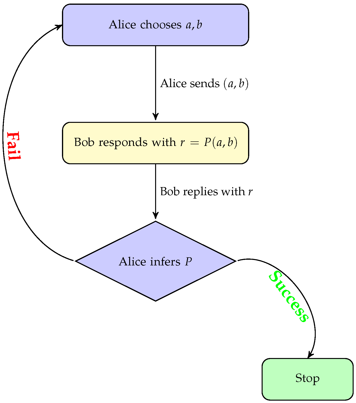
3.2. Defining the Problem

In this subsection, we provide a high-level description of the protocol used to infer the polynomial $P(x,y)$. More precisely, for a given $k\in \mathbb{N}$, Alice (the malicious user) and Bob (the victim) exchange information that can be used by Alice (without Bob’s consent) to compute the polynomial P:

• Bob chooses a polynomial ($P\in G_k$);
• Alice chooses two numbers ($a,b\in {\mathbb{N}}^{*}$) and sends them to Bob;
• Bob computes $r=P(a,b)$ using the values received from Alice, then sends the result to Alice;
• Given r, Alice attempts to infer P from r;
• If Alice is not successful, then she repeats steps 2 and 3 until she accumulates enough data to guess P.

We provide the reader with a graphical representation of the overall process in Figure 1. The objective of our paper is to propose a series of algorithms that solve the problem of inferring P in the aforementioned scenario.

4. Interpolating Bivariate Polynomials

The intuition behind our proposed algorithm (see Algorithm 3) is the following: Alice starts by considering r modulo a. This makes all the $P(a,b)$ terms $c_{i,j}{a}^i{b}^j$ for which $i>0$ vanish. Hence, the positive integer (r) can be regarded as the evaluation modulo (a) of a univariate polynomial:

$$\begin{array}{c}\hfill \sum c_{0,j}{b}^{j}moda.\end{array}$$

Remark 3

(Parameter selection). Note that in the first iteration of the while loop of Algorithm 3, after computing $L_0$,

$$\begin{array}{c}\hfill R_t=\sum _{i,j}{c}_{i,j}{a}^i{b}_t^j=\sum _j{c}_{0,j}{b}_t^j+\sum _{i\ne 0,j}{c}_{i,j}{a}^i{b}_t^j=L_0\left(b\right)+a^d·P^{\prime }(a,b_t).\end{array}$$

When we extract the largest power of a, there is a case in which $d_s$ is larger than the correct exponent (d). That happens when $a|P^{\prime }(a,b_t)$ for all t. This automatically implies that we must have $a\le P^{\prime }(a,b_t)$ for all t due to the construction of $G_k$. Hence, the probability of a not to divide $P^{\prime }(a,b_t)$ for a given t is

$$\begin{array}{c}\hfill 1-\frac{\lfloor \frac{P^{\prime }(a,b_t)}{a}\rfloor }{P^{\prime }(a,b_t)}\ge 1-\frac{P^{\prime }(a,b_t)}{a{P}^{\prime }(a,b_t)}=1-\frac{1}{a}.\end{array}$$

and is non-negligible if a is large enough.

Let $de{g}_b\left(P\right)$ represent the degree of $P\left(x\right)$ with respect to the variable b. When running Algorithm 3, we encounter the following possible cases.

Case 1:

When a is larger than all of P’s coefficients and the number of pairs (n) is equal to $de{g}_b\left(P\right)+1$, the algorithm always outputs the correct polynomial.

Case 2:

When a is less than all of P’s coefficients and the number of pairs (n) is equal to $de{g}_b\left(P\right)+1$, the algorithm outputs a polynomial (P), although not the correct polynomial.

Case 3:

When n is less than $de{g}_b\left(P\right)+1$, it is possible that some of the $R_i$ values (see Algorithm 3) become negative; thus, the algorithm returns ⊥, since it is clear that the computed polynomial is not correct.

Since Alice does not know the exact degree (We do not consider the case of $de{g}_b\left(P\right)=1$, as it is trivial) of P, she uses Algorithm 4 to compute the exact P. Therefore, she avoids Case 3. More precisely, Alice queries Bob until Algorithm 3 returns a polynomial that maps j points into $r_j$ and also satisfies the supplementary condition ($P(a,j+1)=r_j$). This condition is used to avoid the case in which $n\le de{g}_b\left(P\right)$, and all the $R_i$ values become 0. Note that on line 7, we have an additional check in order to avoid the case in which a divides any of P’s coefficients. More precisely, if $j=a+k$, then $j-k$ is not be invertible when computing the ${\ell }_j\left(y\right)$ polynomial.

Example 1.

Let $a=17$ and

$$\begin{array}{c}\hfill P(x,y)=x^{5}y+3x^{3}y+x^2{y}^3+17x{y}^5+15x+y^2+58.\end{array}$$

Note that we are in Case 2. Then, Algorithm 4 returns the following polynomial:

$$\begin{array}{c}\hfill P^{\prime }(x,y)=x^{5}y+3x^{3}y+x^2{y}^5+x^2{y}^3+x^2+x+y^2+7.\end{array}$$

To avoid Case 2, we must query Bob at point $(a^{\prime },1)$, where $a^{\prime }\ne a$, and check if Bob’s answer coincides with the evaluation of the computed polynomial. If the two values do not coincide, then we must run Algorithm 4 with a larger a.

Remark 4.

When working with polynomials from a set ($G_k$), if Alice knows the value of $k\ge 1$, then she can choose $a>2^{2^{k-1}}$ such that the value is a prime number. Otherwise, she chooses a large enough k, and if Algorithm 4 fails, she increases k and tries again until she finds the correct P.

Algorithm 3: Tries to compute a polynomial P such that $r=P(a,b)$.

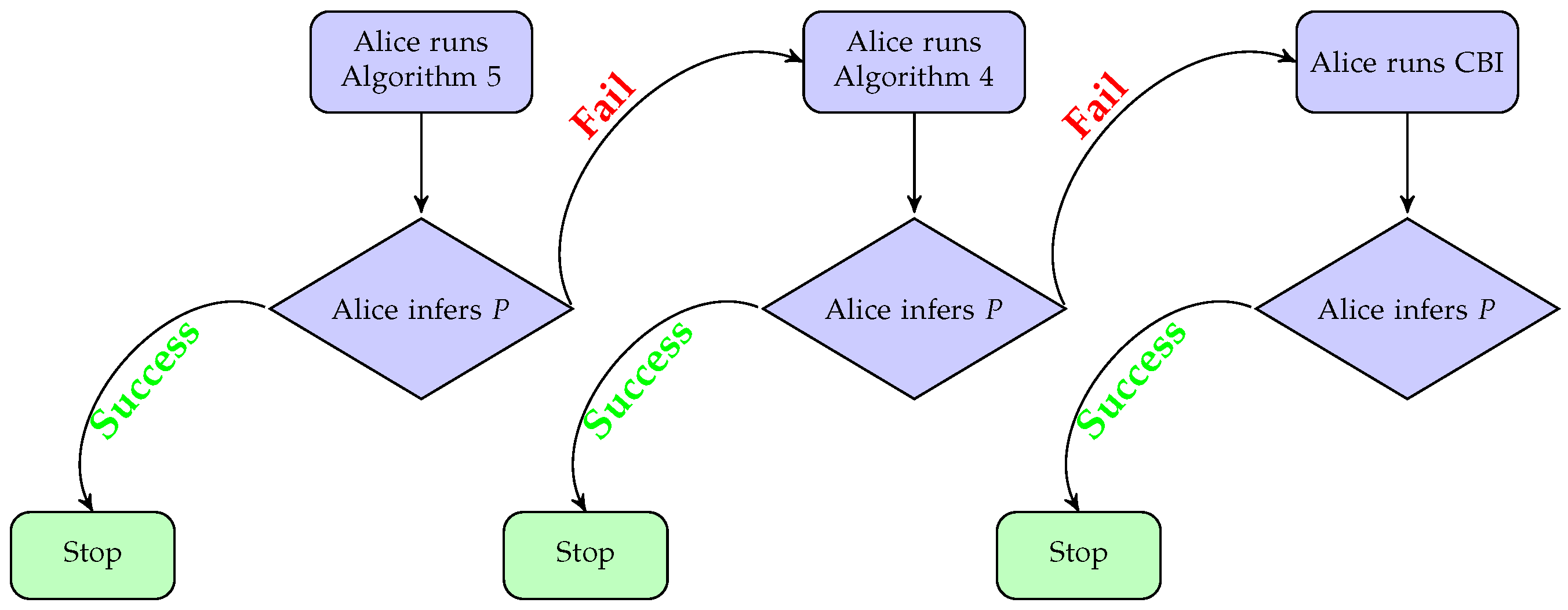
Algorithm 4: Probes Bob until it finds the correct P.

5. Lattice-Based Approaches for Reconstructing Bivariate Polynomials

We consider again $Pmoda$; thus, the positive integer (r) can be regarded as the evaluation modulo (a) of a univariate polynomial:

$$\begin{array}{c}\hfill \sum c_{i,j}{b}^{u_{i,j}}.\end{array}$$

(6)

It can easily be observed that we are tackling a modular knapsack problem that can be solved provided that specific conditions are met (see Section 2). Hence, Alice can use Algorithm 5 to infer P.

If we also restrict k to a value such that $a>2^{2^{k-1}}$, then we are assured that the $c_{i,j}$ values found by solving the modular knapsack are also valid in $\mathbb{Z}$. Hence, the integer value from Equation (6) can be subtracted from r to reveal a polynomial that can be divided by a proper power of a before applying the above process iteratively. When the value zero is reached, the algorithm is run backwards to reconstruct P.

Note that we use the first if of Algorithm 5 for efficiency purposes, given that the modular knapsack resolution algorithm is not needed when $P(x,y)$ does not have monomials only in y.   

Algorithm 5: Tries to compute a polynomial P such that $r=P(a,b)$.

Remark 5

(Parameter selection). As discussed in Section 2, lattice reduction-based algorithms for solving modular knapsacks are suitable in the low-density case (smaller than 1). It is easy to observe that in some cases, we do not fulfill this requirement. More specifically, we consider the case in which $d\ge 1$. Thus, $\frac{2^k}{{log}_2\mathit{max}\left(b_i\right)}\ge 1$. Using Lemma 1, we obtain

$$\begin{array}{c}\hfill 2^k\ge {log}_2\mathit{max}\left(b_i\right)\iff 2^k\ge {log}_2{2}^{2^{k-1}}{\mathit{deg}}_b\left(P\right)\iff \\ \hfill 2^k\ge {log}_2{2}^{2^{k-1}}+{log}_2{\mathit{deg}}_b\left(P\right)\iff 2\ge {log}_{2}2+\frac{{log}_2{\mathit{deg}}_b\left(P\right)}{2^{k-1}}\iff \\ \hfill 1\ge \frac{{log}_2{\mathit{deg}}_b\left(P\right)}{2^{k-1}}\iff 2^{k-1}\ge {log}_2{\mathit{deg}}_b\left(P\right)\end{array}$$

(7)

It follows from Equation (7) that $d\ge 1$ when the number of bits in b is smaller than $\frac{2^{k-1}}{{\mathit{deg}}_b\left(P\right)}$.

Note that in the case of Algorithm 5, the probabilistic argument presented in Remark 3 still holds if a is large enough such that $1/a$ is negligible.

Example 2.

Let $a=913$ and $b=2$.

$$\begin{array}{c}\hfill P(x,y)=2xy+y^2.\end{array}$$

Note that we are in Case 2. Then, Algorithm 5 returns the following polynomial:

$$\begin{array}{c}\hfill P^{\prime }(x,y)=y^2+x{y}^2\end{array}$$

6. Implementation

In order to validate our hypotheses and algorithms, we developed a set of reference implementations (unoptimized versions). We ran the code for Algorithm 4 on a standard desktop using Ubuntu 20.04.5 LTS OS with the following specifications: CPU, Intel i7-4790 4.00 GHz and 16 Gigabytes of RAM. The programming language we used to implement our Lagrange interpolation-based algorithms was Python. We used Mathematica 13.2 online to implement our lattice reduction-based Algorithm 5. Given that our scope was to provide the reader proof-of-concept algorithms for inferring bivariate polynomials of a certain form, we implemented the attack proposed in [31]. Again, we stress that we wish to use modular knapsack resolution algorithms with densities as close to one as possible. The newest developments in the field of lattice reduction [52] are less important for our current work than this aspect, given that researchers’ main struggle is to make algorithms more efficient in terms of complexity.

6.1. Performance Analysis

In

Table 1. Performance analysis for inferring P.

Algorithm	Number of Querries	Complexity
Classical bivariate interpolation [27,38]	$\frac{\left(deg\right(P)+1)\left(deg\right(P)+2)}{2}+1$	$\mathcal{O}\left(deg{\left(P\right)}^4\right)$
Algorithm 4	$de{g}_b\left(P\right)+2$	$\mathcal{O}\left(de{g}_a\left(P\right)de{g}_b\left(P\right)\left(\frac{de{g}_a\left(P\right)}{2}+de{g}_b\left(P\right)\right)\right)$
Algorithm 5	2	$\mathcal{O}\left(de{g}_a\left(P\right)\left(\frac{de{g}_a\left(P\right)}{2}+O\right)\right)$

, we present the number of queries needed to recover the polynomial (P) and the corresponding computational complexity. Note that $deg\left(P\right)$ represents the highest degree of the polynomial ($P\left(x\right)$), while $de{g}_a\left(P\right)$ and $de{g}_b\left(P\right)$ represent the degree of $P\left(x\right)$ with respect to the variables a and b, respectively.

In the case of classical bivariate interpolation, the number of queries differs from that reported in [27,38], since we need an extra point to verify that we deduced the correct P. Note that the extra query is performed to check whether the degree of P is larger than anticipated. Regarding Algorithm 4, if a is larger than the largest coefficient of P, then we need $de{g}_b\left(P\right)+1$ points to recover P and an extra verification point. Lastly, Algorithm 5 only needs a point to infer P and an extra verification point.

To compute the complexity of Algorithm 3, we considered the fact that the complexity of the Lagrange interpolation is $\mathcal{O}\left(de{g}_b{\left(P\right)}^2\right)$ (according to [55]). For our knapsack-based solution (Algorithm 5), we denoted $O=\mathcal{O}\left(\mathcal{A}\right)$, where $\mathcal{A}$ is a modular knapsack resolution algorithm.

6.2. Recommendations

In order to reduce the number of queries to Bob, we recommend first running Algorithm 5 and, if it fails, Algorithm 4. In the improbable case of obtaining the incorrect polynomial, two strategies can be used by Alice: either change a and try again or use a classical bivariate interpolation algorithm (e.g., [38]). A graphical representation of the recommended process is provided in Figure 2, where CBI denotes a classical bivariate interpolation algorithm.

7. Conclusions

The main focus of this paper is the problem of inferring bivariate polynomials with a specific form required for homomorphic encryption. To solve this problem, we propose two methods. The first method is based on Lagrange interpolation, which is a well-known technique for polynomial evaluation. The second method is based on modular knapsack resolution algorithms, which are commonly used in cryptography to solve similar problems. Additionally, this paper offers guidance with respect to how to use these algorithms to achieve improved accuracy. This guidance may be useful for practitioners who wish to apply these algorithms in real-world scenarios.

Future Work

An interesting research direction would be to extend our proposed methods to multivariate polynomials and to look into other ways of solving the problem of inferring polynomials. For example, the PSLQ algorithm introduced in [56] is a method of finding integer relations. In certain cases, PSLQ might be significantly better than some of the algorithms based on lattice reduction in terms of implementation performance and precision.

Using artificial intelligence techniques to obtain improved solutions is a generally applied strategy. However, such ideas are beyond the scope of our paper, and we leave them for future work.

References

1. Dertouzos, M.L.; Rivest, R.L.; Adleman, L. On Data Banks and Privacy Homomorphisms. In Foundations of Secure Computation; Academia Press: Cambridge, MA, USA, 1978; pp. 169–179. [Google Scholar]
2. Rivest, R.L.; Shamir, A.; Adleman, L. A Method for Obtaining Digital Signatures and Public-Key Cryptosystems. Commun. ACM 1978, 21, 120–126. [Google Scholar] [CrossRef] [Green Version]
3. Gentry, C. A Fully Homomorphic Encryption Scheme. Ph.D. Thesis, Stanford University, Stanford, CA, USA, 2009. [Google Scholar]
4. van Dijk, M.; Gentry, C.; Halevi, S.; Vaikuntanathan, V. Fully Homomorphic Encryption over the Integers. In Proceedings of the EUROCRYPT’10; Lecture Notes in Computer Science; Springer: Berlin/Heidelberg, Germany, 2010; Volume 6110, pp. 24–43. [Google Scholar]
5. Brakerski, Z.; Gentry, C.; Vaikuntanathan, V. Fully Homomorphic Encryption without Bootstrapping. Cryptology ePrint Archive, Paper 2011/277. 2011. Available online: https://eprint.iacr.org/2011/277.pdf (accessed on 25 May 2023).
6. Fan, J.; Vercauteren, F. Somewhat Practical Fully Homomorphic Encryption. Cryptology ePrint Archive, Paper 2012/144. 2012. Available online: https://eprint.iacr.org/2012/144.pdf (accessed on 25 May 2023).
7. Brakerski, Z. Fully Homomorphic Encryption without Modulus Switching from Classical GapSVP. In Proceedings of the CRYPTO’12; Lecture Notes in Computer Science; Springer: Berlin/Heidelberg, Germany, 2012; Volume 7417, pp. 868–886. [Google Scholar]
8. Bos, J.W.; Lauter, K.E.; Loftus, J.; Naehrig, M. Improved Security for a Ring-Based Fully Homomorphic Encryption Scheme. In Proceedings of the IMACC’13; Lecture Notes in Computer Science; Springer: Berlin/Heidelberg, Germany, 2013; Volume 8308, pp. 45–64. [Google Scholar]
9. Gentry, C.; Sahai, A.; Waters, B. Homomorphic Encryption from Learning with Errors: Conceptually-Simpler, Asymptotically-Faster, Attribute-Based. In Proceedings of the CRYPTO’13; Lecture Notes in Computer Science; Springer: Berlin/Heidelberg, Germany, 2013; Volume 8042, pp. 75–92. [Google Scholar]
10. Brakerski, Z.; Vaikuntanathan, V. Lattice-Based FHE as Secure as PKE. In Proceedings of the ITCS’14; Association for Computing Machinery: New York, NY, USA, 2014; pp. 1–12. [Google Scholar]
11. Carpov, S.; Chillotti, I.; Gama, N.; Georgieva, M.; Izabachene, M. TFHE: Fast Fully Homomorphic Encryption Library. 2016. Available online: https://tfhe.github.io/tfhe (accessed on 25 May 2023).
12. Cheon, J.H.; Kim, A.; Kim, M.; Song, Y.S. Homomorphic Encryption for Arithmetic of Approximate Numbers. In Proceedings of the ASIACRYPT’17; Lecture Notes in Computer Science; Springer: Berlin/Heidelberg, Germany, 2017; Volume 10624, pp. 409–437. [Google Scholar]
13. Li, B.; Micciancio, D. On the Security of Homomorphic Encryption on Approximate Numbers. In Proceedings of the EUROCRYPT’21; Lecture Notes in Computer Science; Springer: Berlin/Heidelberg, Germany, 2021; Volume 12696, pp. 648–677. [Google Scholar]
14. A Curated List of Amazing Homomorphic Encryption Libraries, Software and Resources. 2023. Available online: https://github.com/jonaschn/awesome-he (accessed on 25 May 2023).
15. Williams, E.A. Driven by Privacy, Homomorphic Encryption Is Changing the Way We Do Business. 2021. Available online: https://www.forbes.com/sites/forbestechcouncil/2021/05/19/driven-by-privacy-homomorphic-encryption-is-changing-the-way-we-do-business/?sh=60d688004cbf (accessed on 25 May 2023).
16. Jackson, A. 20 Use Cases of Homomorphic Encryption Every CISO Must Know. 2023. Available online: https://www.linkedin.com/pulse/20-use-cases-homomorphic-encryption-every-ciso-must-know-jackson-/ (accessed on 25 May 2023).
17. Bos, J.W.; Lauter, K.; Naehrig, M. Private Predictive Analysis on Encrypted Medical Data. J. Biomed. Inform. 2014, 50, 234–243. [Google Scholar] [CrossRef] [PubMed] [Green Version]
18. Zhang, C.; Zhu, L.; Xu, C.; Lu, R. PPDP: An Efficient and Privacy-Preserving Disease Prediction Scheme in Cloud-Based e-Healthcare System. Future Gener. Comput. Syst. 2018, 79, 16–25. [Google Scholar] [CrossRef]
19. Munjal, K.; Bhatia, R. A Systematic Review of Homomorphic Encryption and its Contributions in Healthcare Industry. Complex Intell. Syst. 2022, 1–28. [Google Scholar] [CrossRef] [PubMed]
20. Ayday, E. Cryptographic Solutions for Genomic Privacy. In Proceedings of the FC 2016; Lecture Notes in Computer Science; Springer: Berlin/Heidelberg, Germany, 2016; Volume 9604, pp. 328–341. [Google Scholar]
21. Graepel, T.; Lauter, K.; Naehrig, M. ML Confidential: Machine Learning on Encrypted Data. In Proceedings of the ICISC 2012; Lecture Notes in Computer Science; Springer: Berlin/Heidelberg, Germany, 2012; Volume 7839, pp. 1–21. [Google Scholar]
22. Cheon, J.H.; Jeong, J.; Lee, J.; Lee, K. Privacy-Preserving Computations of Predictive Medical Models with Minimax Approximation and Non-Adjacent Form. In Proceedings of the FC 2017; Lecture Notes in Computer Science; Springer: Berlin/Heidelberg, Germany, 2017; Volume 10323, pp. 53–74. [Google Scholar]
23. Marcolla, C.; Sucasas, V.; Manzano, M.; Bassoli, R.; Fitzek, F.H.; Aaraj, N. Survey on Fully Homomorphic Encryption, Theory, and Applications. Proc. IEEE 2022, 110, 1572–1609. [Google Scholar] [CrossRef]
24. Derler, D.; Ramacher, S.; Slamanig, D. Homomorphic Proxy Re-Authenticators and Applications to Verifiable Multi-User Data Aggregation. In Proceedings of the FC 2017; Lecture Notes in Computer Science; Springer: Berlin/Heidelberg, Germany, 2017; Volume 10322, pp. 124–142. [Google Scholar]
25. Diallo, M.H.; August, M.; Hallman, R.; Kline, M.; Au, H.; Beach, V. CallForFire: A Mission-Critical Cloud-Based Application Built Using the Nomad Framework. In Proceedings of the FC 2016; Lecture Notes in Computer Science; Springer: Berlin/Heidelberg, Germany, 2016; Volume 9604, pp. 319–327. [Google Scholar]
26. Doröz, Y.; Çetin, G.S.; Sunar, B. On-the-fly Homomorphic Batching/Unbatching. In Proceedings of the FC 2016; Lecture Notes in Computer Science; Springer: Berlin/Heidelberg, Germany, 2016; Volume 9604, pp. 288–301. [Google Scholar]
27. Kincaid, D.; Kincaid, D.R.; Cheney, E.W. Numerical Analysis: Mathematics of Scientific Computing; American Mathematical Society: Providence, RI, USA, 2009; Volume 2. [Google Scholar]
28. Lagarias, J.C.; Odlyzko, A.M. Solving Low-Density Subset Sum Problems. J. ACM 1985, 32, 229–246. [Google Scholar] [CrossRef]
29. Coster, M.J.; Joux, A.; LaMacchia, B.A.; Odlyzko, A.M.; Schnorr, C.P.; Stern, J. Improved Low-Density Subset Sum Algorithms. Comput. Complex. 1992, 2, 111–128. [Google Scholar] [CrossRef] [Green Version]
30. Howgrave-Graham, N.; Joux, A. New Generic Algorithms for Hard Knapsacks. In Proceedings of the EUROCRYPT’10; Gilbert, H., Ed.; Springer: Berlin/Heidelberg, Germany, 2010; pp. 235–256. [Google Scholar]
31. Becker, A.; Coron, J.S.; Joux, A. Improved Generic Algorithms for Hard Knapsacks. In Proceedings of the EUROCRYPT’11; Lecture Notes in Computer Science; Springer: Berlin/Heidelberg, Germany, 2011; pp. 364–385. [Google Scholar]
32. Nguyen, P.Q.; Stehlé, D. An LLL Algorithm with Quadratic Complexity. SIAM J. Comput. 2009, 39, 874–903. [Google Scholar] [CrossRef] [Green Version]
33. Kirchner, P.; Espitau, T.; Fouque, P.A. Towards Faster Polynomial-Time Lattice Reduction. In Proceedings of the CRYPTO’21; Lecture Notes in Computer Science; Springer: Berlin/Heidelberg, Germany, 2021; Volume 12826, pp. 760–790. [Google Scholar]
34. Koy, H.; Schnorr, C.P. Segment LLL-Reduction of Lattice Bases. In Proceedings of the Cryptography and Lattices; Springer: Berlin/Heidelberg, Germany, 2001; pp. 67–80. [Google Scholar]
35. Schnorr, C.P. Fast LLL-type lattice reduction. Inf. Comput. 2006, 204, 1–25. [Google Scholar] [CrossRef] [Green Version]
36. Nguyen, P.Q.; Stern, J. Adapting Density Attacks to Low-Weight Knapsacks. In Proceedings of the ASIACRYPT; Lecture Notes in Computer Science; Springer: Berlin/Heidelberg, Germany, 2005; Volume 3788, pp. 41–58. [Google Scholar]
37. Micchelli, C.A. Algebraic Aspects of Interpolation. In Proceedings of Symposia in Applied Mathematics; AMS: New York, NY, USA, 1986; Volume 36, pp. 81–102. [Google Scholar]
38. Saniee, K. A Simple Expression for Multivariate Lagrange Interpolation. SIAM Undergrad. Res. Online 2008, 1, 1–9. [Google Scholar] [CrossRef]
39. Garey, M.R.; Johnson, D.S. Computers and Intractability; A Guide to the Theory of NP-Completeness; W. H. Freeman & Co.: New York, NY, USA, 1990. [Google Scholar]
40. Martello, S.; Toth, P. Knapsack Problems: Algorithms and Computer Implementations; John Wiley & Sons, Inc.: Hoboken, NJ, USA, 1990. [Google Scholar]
41. Merkle, R.; Hellman, M. Hiding Information and Signatures in Trapdoor Knapsacks. IEEE Trans. Inf. Theory 1978, 24, 525–530. [Google Scholar] [CrossRef] [Green Version]
42. Naccache, D.; Stern, J. A New Public-Key Cryptosystem. In Proceedings of the EUROCRYPT ’97; Lecture Notes in Computer Science; Springer: Berlin/Heidelberg, Germany, 1997; Volume 1233, pp. 27–36. [Google Scholar]
43. Salomaa, A. A Deterministic Algorithm for Modular Knapsack Problems. Theor. Comput. Sci. 1991, 88, 127–138. [Google Scholar] [CrossRef] [Green Version]
44. Chee, Y.M.; Joux, A.; Stern, J. The Cryptanalysis of a New Public-Key Cryptosystem Based on Modular Knapsacks. In Proceedings of the CRYPTO’91; Lecture Notes in Computer Science; Springer: Berlin/Heidelberg, Germany, 1991; Volume 576, pp. 204–212. [Google Scholar]
45. Hoffstein, J.; Pipher, J.; Silverman, J. An Introduction to Mathematical Cryptography; Undergraduate Texts in Mathematics; Springer: Berlin/Heidelberg, Germany, 2008. [Google Scholar]
46. Anzala-Yamajako, A. Review of Algorithmic Cryptanalysis, by Antoine Joux. SIGACT News 2012, 43, 13–16. [Google Scholar] [CrossRef]
47. Lenstra, A.; Lenstra, H.; Lovász, L. Factoring polynomials with rational coefficients. Math. Ann. 1982, 261, 515–534. [Google Scholar] [CrossRef]
48. Schroeppel, R.; Shamir, A. A T = O(2n/2), S = O(2n/4) Algorithm for Certain NP-Complete Problems. SIAM J. Comput. 1981, 10, 456–464. [Google Scholar] [CrossRef]
49. Schnorr, C. A Hierarchy of Polynomial Time Lattice Basis Reduction Algorithms. Theor. Comput. Sci. 1987, 53, 201–224. [Google Scholar] [CrossRef] [Green Version]
50. fpLLL. 2022. Available online: https://github.com/fplll/fplll (accessed on 25 May 2023).
51. Kirchner, P.; Espitau, T.; Fouque, P.A. Fast Reduction of Algebraic Lattices over Cyclotomic Fields. In Proceedings of the CRYPTO’20; Lecture Notes in Computer Science; Springer: Berlin/Heidelberg, Germany, 2020; Volume 12171, pp. 155–185. [Google Scholar]
52. Ryan, K.; Heninger, N. Fast Practical Lattice Reduction through Iterated Compression. Cryptology ePrint Archive, Paper 2023/237. 2023. Available online: https://eprint.iacr.org/2023/237 (accessed on 25 May 2023).
53. Aho, A.; Sloane, N. Some Doubly Exponential Sequences. Fibonacci Q. 1973, 11, 429–437. [Google Scholar]
54. Sequence A007018. Available online: https://oeis.org/A007018 (accessed on 25 May 2023).
55. Press, W.H.; Teukolsky, S.A.; Vetterling, W.T.; Flannery, B.P. Numerical Recipes: The Art of Scientific Computing; Cambridge University Press: Cambridge, UK, 2007. [Google Scholar]
56. Ferguson, H.R.P.; Bailey, D.H.; Kutler, P. A Polynomial Time, Numerically Stable Integer Relation Algorithm; NASA Technical Report RNR–91–032. 1991. Available online: https://ntrs.nasa.gov/citations/20020052399 (accessed on 25 May 2023).
Figure 1. The overall process.
Cryptography 07 00031 g001
Figure 2. The recommended process.
Cryptography 07 00031 g002