Selection Strategy of F4-Style Algorithm to Solve MQ Problems Related to MPKC

Abstract

Multivariate public-key cryptosystems are potential candidates for post-quantum cryptography. The security of multivariate public-key cryptosystems relies on the hardness of solving a system of multivariate quadratic polynomial equations. Faugère’s F4 algorithm is one of the solution techniques based on the theory of Gröbner bases and selects critical pairs to compose the Macaulay matrix. Reducing the matrix size is essential. Previous research has not fully examined how many critical pairs it takes to reduce to zero when echelonizing the Macaulay matrix in rows. Ito et al. (2021) proposed a new critical-pair selection strategy for solving multivariate quadratic problems associated with encryption schemes. Instead, this paper extends their selection strategy for solving the problems associated with digital signature schemes. Using the OpenF4 library, we compare the software performance between the integrated F4-style algorithm of the proposed methods and the original F4-style algorithm. Our experimental results demonstrate that the proposed methods can reduce the processing time of the F4-style algorithm by up to a factor of about seven under certain specific parameters. Moreover, we compute the minimum number of critical pairs to reduce to zero and propose their extrapolation outside our experimental scope for further research.

1. Introduction

Shor demonstrated that solving both the integer factorization problem (IFP) and the discrete logarithm problem (DLP) is theoretically tractable in polynomial time [1]. Both Rivest–Shamir–Adleman (RSA) public-key cryptography and elliptic curve cryptography (ECC) are widely used, and their security depends on the IFP and DLP, respectively. In recent years, research and development of quantum computers have progressed rapidly. For example, noisy intermediate-scale quantum computers are already in practical use. Since system migration takes time in general, preparation for migration to PQC is a significant issue. Research, development, and standardization projects for post-quantum cryptography (PQC) are ongoing within these contexts. The PQC standardization process was started by the National Institute of Standards and Technology (NIST) in 2016 [2]. Several cryptosystems have been proposed for the NIST PQC project, including lattice-based, code-based, and hash-based cryptosystems. The multivariate public-key cryptosystem (MPKC) is one of the cryptosystems proposed for the NIST PQC project. At the end of the third round, NIST selected four candidates to be standardized, as shown in

Table 1. NIST Selected Algorithms 2022.

Functionality	Algorithm	Underlying Security Problems
Public-key Encryption and Key-establishment Algorithms	CRYSTALS-KYBER [4]	Lattice-based
Digital signatures	CRYSTALS-Dilithium [4]	Lattice-based
	FALCON [5]	Lattice-based
	SPHINCS${}^{+}$ [6]	Hash-based

, and moved four candidates to the fourth-round evaluation, as shown in

Table 2. NIST Round-Four Submissions.

Functionality	Algorithm	Underlying Security Problems
Digital signatures	BIKE [7]	Lattice-based
	Classic McEliece [8]	Code-based
	HQC [9]	Code-based
	SIKE *	Isogeny-based

* Castryck and Decru found that SIKE is insecure [10,11].

. Moreover, NIST issued a request for proposals of digital signature schemes with short signatures and fast verification [3]. MPKCs are often more efficient than other public-key cryptosystems, primarily digital signature schemes, as described in the subsequent paragraph; therefore, researching the security of MPKCs is still important.

An MPKC is basically an asymmetric cryptosystem that has a trapdoor one-way multivariate (quadratic) polynomial map $\mathcal{F}$ over a finite field ${\mathbb{F}}_q$. Let $\mathcal{F}$: ${\mathbb{F}}_q^n\to {\mathbb{F}}_q^m$ a (quadratic) polynomial map whose inverse can be computed easily, and two randomly selected invertible affine linear maps $\mathcal{S}:{\mathbb{F}}_q^n\to {\mathbb{F}}_q^n$ and $\mathcal{T}:{\mathbb{F}}_q^m\to {\mathbb{F}}_q^m$. The secret key consists of $\mathcal{F}$, $\mathcal{S}$, and $\mathcal{T}$. The public key consists of the composite map $\mathcal{P}$: ${\mathbb{F}}_q^n\to {\mathbb{F}}_q^m$ such that $\mathcal{P}=\mathcal{T}\circ \mathcal{F}\circ \mathcal{S}$. The public key can be regarded as a set $\mathcal{P}$ of m (quadratic) polynomials in n variables:

$$\mathcal{P}=\left(p_1\left(x_1,\dots ,x_n\right),\dots ,p_m\left(x_1,\dots ,x_n\right)\right):{\mathbb{F}}_q^n\to {\mathbb{F}}_q^m,$$

where each $p_i$ is a non-linear (quadratic) polynomial.

Multivariate quadratic (MQ) problem: Find a solution $x=\left(x_1,\dots ,x_n\right)\in {\mathbb{F}}_q^n$ such that the system of (quadratic) polynomial equations: $p_1\left(x\right)=\cdots =p_m\left(x\right)=0.$

Then, the MQ problem is closely related to the attack that forges signatures for the MPKC.

Isomorphism of polynomials (IP) problem: Let $\mathcal{A}$ and $\mathcal{B}$ be two polynomial maps from ${\mathbb{F}}_q^n$ to ${\mathbb{F}}_q^m$. Find two invertible affine linear maps $\mathcal{S}$: ${\mathbb{F}}_q^n\to {\mathbb{F}}_q^n$ and $\mathcal{T}$: ${\mathbb{F}}_q^m\to {\mathbb{F}}_q^m$ such that $\mathcal{B}=\mathcal{T}\circ \mathcal{A}\circ \mathcal{S}$.

Then, the IP problem is closely related to the attack for finding secret keys for the MPKC.

One of the most well-known public-key cryptosystems based on multivariate polynomials over a finite field was proposed by Matsumoto and Imai [12]. Patarin [13] later demonstrated that the Matsumoto–Imai cryptosystem is insecure, proposed the hidden field equation (HFE) public-key cryptosystem by repairing their cryptosystems [14] and designed the Oil and Vinegar (OV) scheme [15]. There are several variations of the HFE and OV schemes, e.g., Kipnis et al. proposed the unbalanced OV (UOV) scheme [16] as described in Section 2.5.

Several MPKCs were proposed for the NIST PQC project [17], e.g., GeMSS [18], LUOV [19], MQDSS [20], and Rainbow [21] MPKCs. Ding et al. found a forgery attack on LUOV [22], and Kales and Zaverucha found a forgery attack on MQDSS [23]. At the end of the second round, NIST selected Rainbow as a third-round finalist and moved GeMSS to an alternate candidate [24].

MinRank problem: Let r be a positive integer and k matrices $M_1,\dots ,M_k\in {\mathbb{F}}_q^{m\times n}$. Find $x_1,\dots ,x_k\in {\mathbb{F}}_q$ such that $\left(x_1,\dots ,x_k\right)\ne 0$ and

$$\mathrm{Rank}\left(\sum _{i=1}^k{x}_i{M}_i\right)\le r.$$

The MinRank problem can be reduced to the MQ problem [25,26,27]. By solving the MinRank problem, Tao et al. found a key recovery attack on GeMSS [28], and Beullens found a key recovery attack on Rainbow [29,30].

NIST reported that a third-round finalist of the digital signature scheme, Rainbow, had the property that its signing and verification were efficient, and the signature size was very short [31]. Beullens et al. also demonstrated that the (U)OV scheme performed comparably to the algorithms selected by NIST [32].

As noted above, the security of an MPKC is highly dependent on the hardness of the MQ problem because multivariate polynomial equations are transformed into MQ polynomial equations by increasing the number of variables and equations. To break a cryptosystem, we translate its underlying algebraic structure into a system of multivariate polynomial equations. There are three well-known algebraic approaches to solving the MQ problem: the extended linearization (XL) algorithm proposed by Courtois et al. [33] and the F4 and F5 algorithms proposed by Faugère [34,35]. The XL algorithm is described in Section 2.2. Gröbner bases algorithm is described in Section 2.3 and Section 3.1 and the F4 algorithm is described in Section 3.2.

In addition to the theoretical evaluations of the computational complexity, practical evaluations are also crucial in the research of cryptography, e.g., such as many efforts addressing the RSA [36], ECC [37], and Lattice challenges [38]. The Fukuoka MQ challenge project [39,40] was started in 2015 to evaluate the security of the MQ problem. In this project, the MQ problems were classified into encryption and digital signature schemes. Each scheme was then classified into three categories according to the number of quadratic equations (m), the number of variables (n), and the characteristic of the finite field. The encryption schemes were classified into types I to III, which correspond to the condition where $m=2n$ over ${\mathbb{F}}_2$, ${\mathbb{F}}_{256}$, and ${\mathbb{F}}_{31}$, respectively. The digital-signature schemes were classified into types IV to VI, which correspond to the condition where $n\approx 1.5m$ over ${\mathbb{F}}_2$, ${\mathbb{F}}_{256}$, and ${\mathbb{F}}_{31}$, respectively. Up to the time of writing this paper, all the best records in the Fukuoka MQ challenge, except type IV, have been set by variant algorithms of both the XL and F4 algorithms. For example, the authors improved the F4-style algorithm and set new records of both type II and III, as described below, but a variant of the XL algorithm later surpassed the record of type III.

The F4 algorithm proposed by Faugère is an improvement of Buchberger’s algorithm for computing Gröbner bases [41,42], as described in Section 3.2. In Buchberger’s algorithm, it is fundamental to compute the S-polynomial of two polynomials, as described in Section 3.1. The critical pair is defined by a set of data (two polynomials, the least common multiple ($\mathrm{LCM}$) of their leading terms, and two associated monomials required to compute the S-polynomial, as described in Section 2.3. The F4 algorithm computes many S-polynomials simultaneously using Gaussian elimination. A variant of the F4 algorithm involving these matrix operations is referred to as an F4-style algorithm in this paper. There are several variants of the F4-style algorithm. For example, Joux and Vitse [43] designed an efficient variant algorithm to compute Gröbner bases for similar polynomial systems. Additionally, Makarim and Stevens [44] proposed a variant M4GB algorithm that could reduce the leading and lower terms of a polynomial. Using the M4GB algorithm, they set the best record for the Fukuoka MQ challenge of type VI with up to 20 equations ($m=20$), at the time of writing this paper.

Recently, Ito et al. [45] also proposed a variant algorithm that could solve the Fukuoka MQ challenge for both types II and III, with up to 37 equations ($m=37$), and set the best record of type II at the time of writing. In their paper, the following selection strategy for critical pairs was proposed: (a) a set of critical pairs is partitioned into smaller subsets $C_1,\dots ,C_k$ such that $|C_i|=256$$(1\le i\le k-1)$; (b) Gaussian elimination is performed for an associated Macaulay matrix composed of each subset; and (c) the remaining subsets are omitted if some S-polynomials are reduced to zero. Herein, we refer to the subdividing method as (a) and the removal method as (c). Their strategy was then validated only under the following two situations: systems of MQ polynomial equations associated with encryption schemes, i.e., the $m=2n$ case and the $|C_i|=256$ case. Thus, in this paper, we propose several types of partitions related to the subdividing method and focus on their validity for solving systems of MQ polynomial equations associated with digital-signature schemes, i.e., the $n>m$ case. We evaluate the performance of the proposed methods for the $m=n+1$ case only because we focus on evaluating the performance of the proposed methods. In other words, before executing the F4-style algorithm combined with the proposed methods, we assume that random values or specific values have already been substituted for some $n-m+1$ variables in the system, according to the hybrid approach [46].

Our contribution. In general, the size of a matrix affects the computational complexity of Gaussian elimination. Reducing the number of critical pairs is essential because they determine the size of the Macauley matrix. First, we propose three basic subdividing methods SD1, SD2, and SD3, which have different types of partitions for a set of critical pairs. Then, we integrate both the proposed subdividing methods and the removal method into the OpenF4 library [47] and compare their software performance with that of the original library using similar settings to those of types V and VI of the Fukuoka MQ challenge, i.e., $(n,m)=(9,10),\dots ,(15,16)$ over ${\mathbb{F}}_{256}$ and $(n,m)=(9,10),\dots ,(16,17)$ over ${\mathbb{F}}_{31}$. To validate the removal method, we then verify that neither a temporary base nor critical pair of a higher degree arises from unused critical pairs in omitted subsets. Here, $D_{\max }$ denotes the highest degree of critical pairs appearing in the Gröbner bases computation or the F4-style algorithm. The process by which the degree of a critical pair reaches $D_{\max }$ for the first time is referred to as the first half, and the remaining process is referred to as the second half. Then, our experiments show that a combination of two different basic methods (i.e., SD3 followed by SD1) is faster than all other methods because of the difference between the first and second halves of the computation. 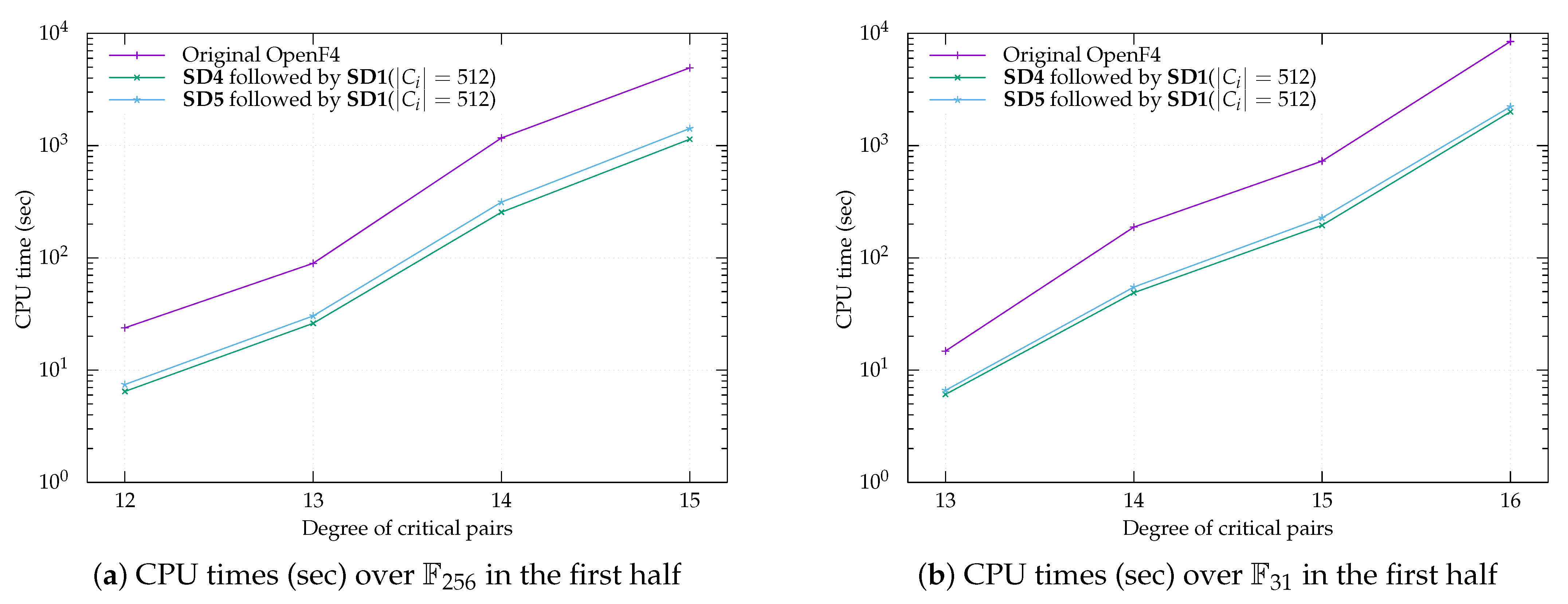Finally, our experiments show that the number of critical pairs that generate a reduction to zero for the first time is approximately constant under the condition where $m=n+1$ in the sense that a similar number is obtained with a high probability. We also propose two derived subdividing methods (SD4 and SD5) for the first half. The experimental results show that SD4 followed by SD1 is the fastest method and SD5 is as fast as SD4, as long as $n<16$ over ${\mathbb{F}}_{256}$ and $n<17$ over ${\mathbb{F}}_{31}$ hold. Moreover, we propose an extrapolation outside the scope of the experiments for further research. Our findings make a unique contribution toward improving the security evaluation of MPKC.

Organization. The remainder of this paper is organized as follows. First, we introduce basic notations and preliminaries in Section 2. Next, we present background to Gröbner bases computation in Section 3. Then, we describe the proposed method in Section 3.4. Afterward, we present the performance result of the proposed method in Section 4. Finally, the paper is concluded in Section 5.

2. Preliminaries

In the following, we define the notations and terminology used in this paper.

2.1. Notations

Let $\mathbb{N}$ be the set of all natural numbers, $\mathbb{Z}$ the set of all integers, ${\mathbb{Z}}_{\ge 0}$ the set of all non-negative integers, and ${\mathbb{F}}_q$ a finite field with q elements. $\mathcal{R}$ denotes a polynomial ring of n variables over ${\mathbb{F}}_q$, i.e., $\mathcal{R}={\mathbb{F}}_q[x_1,\dots ,x_n]={\mathbb{F}}_q\left[x\right]$.

A monomial $x^a$ is defined by a product $x_1^{a_1}\cdots x_n^{a_n}$, where the $a=(a_1,\dots ,a_n)$ is an element of ${\mathbb{Z}}_{\ge 0}^n$. Furthermore, $\mathcal{M}$ denotes the set of all monomials in $\mathcal{R}$, i.e., $\mathcal{M}=\{x_1^{a_1}\cdots x_n^{a_n}\mid a_1,\dots ,a_n\in {\mathbb{Z}}_{\ge 0}\}$. For $c\in {\mathbb{F}}_q$ and $u\in \mathcal{M}$, we call the product $cu$ a term and c the coefficient of u. $\mathcal{T}$ denotes the set of all terms, i.e., $\mathcal{T}=\{cu\mid c\in {\mathbb{F}}_q,u\in \mathcal{M}\}$. For a polynomial, $f={\sum }_i{c}_i{u}_i\in \mathcal{R}$ for $c_i\in {\mathbb{F}}_q\backslash \left\{0\right\}$ and $u_i\in \mathcal{M}$, $\mathcal{T}\left(f\right)$ denotes the set $\left\{c_i{u}_i\right\}$, and $\mathcal{M}\left(f\right)$ denotes the set $\left\{u_i\right\}$.

The total degree of $x^a$ is defined by the sum $a_1+\cdots +a_n$, which is denoted by $deg\left(x^a\right)$. The total degree of f is defined by $max\{deg(u)\mid u\in \mathcal{M}(f\left)\right\}$ and is denoted by $deg\left(f\right)$.

Definition 1.

A total order ≺ on $\mathcal{M}$ is called a monomial order if the following conditions hold:

(i)

s, t, $u\in \mathcal{M}$, t ⪯ s ⇒ $ut$ ⪯ $us$,

(ii)

∀$t\in \mathcal{M}$, 1 ⪯ t.

Here, if $s\prec t$ or $s=t$ holds, then we denote $s⪯t$.

Definition 2.

The degree reverse lexicographical order ≺ is defined by

$$\begin{array}{cc}\hfill & x_1^{a_1}\cdots x_n^{a_n}\prec x_1^{b_1}\cdots x_n^{b_n}\hfill \\ \hfill & \iff \left\{\begin{array}{c}{a}_1+\cdots +a_n<b_1+\cdots +b_n\hfill \\ or\hfill \\ a_1+\cdots +a_n=b_1+\cdots +b_n\mathrm{and}\exists ks.t.a_k>b_k\mathit{and}\forall l(l>k)s.t.a_l=b_l.\hfill \end{array}\right.\hfill \end{array}$$

For example, in $\mathcal{R}[x_1,x_2,x_3]$,

$$1\prec x_3\prec x_2\prec x_1\prec x_3^2\prec x_2{x}_3\prec x_1{x}_3\prec x_2^2\prec x_1{x}_2\prec x_1^2\prec x_3^3\prec \cdots .$$

The degree reverse lexicographical order ≺ is fixed throughout this paper as a monomial order.

For a polynomial $f\in \mathcal{R}$, $\mathrm{LM}\left(f\right)$ denotes the leading monomial of f, i.e., $\mathrm{LM}\left(f\right)={max}_{\prec }\mathcal{M}\left(f\right)$, and $\mathrm{LT}\left(f\right)$ denotes the leading term of f, i.e., $\mathrm{LT}\left(f\right)={max}_{\prec }\mathcal{T}\left(f\right)$. In addition, $\mathrm{LC}\left(f\right)$ denotes the corresponding coefficient for $\mathrm{LT}\left(f\right)$. A polynomial f is called monic if $\mathrm{LC}\left(f\right)=1$.

For a subset $F\subset \mathcal{R}$, $\mathrm{LM}\left(F\right)$ denotes the set of leading monomials of polynomials $f\in F$, i.e., $\mathrm{LM}\left(F\right)=\left\{\mathrm{LM}\right(f)\mid f\in F\}$.

For two monomials $x^a=x_1^{a_1}\dots x_n^{a_n}$ and $x^b=x_1^{b_1}\dots x_n^{b_n}$ where $a=(a_1,\dots ,a_n)$ and $b=(b_1,\dots ,b_n)\in {\mathbb{Z}}_{\ge 0}^n$, their corresponding least common multiple (LCM) and the greatest common divisor (GCD) are defined as $\mathrm{LCM}(x^a,x^b)=x^c$ where $c=(max(a_1,b_1),\dots ,$$max(a_n,b_n))$, and $\mathrm{GCD}(x^a,x^b)=x^c$ where $c=(min(a_1,b_1),\dots ,min(a_n,b_n))$.

For two subsets A and B, $A\prec B$ is defined if $a\prec b$ holds for $a\in A$ and $b\in B$.

2.2. The XL Algorithm

Let D be the parameter of the XL algorithm. Let $\{p_1,\dots ,p_m\}$ be a set of polynomials over a finite field ${\mathbb{F}}_q$. The XL algorithm executes the following steps:

• Multiply: Generate all the products (${\prod }_{j=1}^k{x}_{i_j}$) $p_i$ with $k\le D-deg\left(p_i\right)$.
• Multiply: Consider each monomial in $x_i$ of degree $\le D$ as a new variable and perform Gaussian elimination on the linear equation obtained in step 1. The ordering on the monomials must be such that all the terms containing one variables (say $x_1$) are eliminated last.
• Solve: Assume that step 2 yields at least one univariate equation in the power of $x_1$. Solve this equation over ${\mathbb{F}}_q$.
• Repeat: Simplify the equations and repeat the process to find the values of the other variables.

Step 1 is regarded as the construction of the Macaulay matrix with the ordering specified in step 2, as described in Section 3.2. It is difficult to estimate the parameter D in advance. The computational complexity of the XL algorithm is roughly

$$\mathcal{O}\left({\left(\genfrac{}{}{0pt}{}{n+D}{D}\right)}^{\omega }\right),$$

where n is the number of variables and $2<\omega \le 3$ is the linear algebra constant [48].

2.3. Gröbner Bases

The concept of Gröbner bases was introduced by Buchberger [49] in 1979. Computing Gröbner bases is a standard tool for solving simultaneous equations. This section presents the definitions and notations used in Gröbner bases. Methods to compute Gröbner bases are explained in Section 3.

Here, $\langle G\rangle$ denotes an ideal generated by a subset $G\subset \mathcal{R}$. $G\subset I$ is called a basis of an ideal I if $I=\langle G\rangle$ holds. We refer to G as Gröbner bases of I if for all $f\in I$ there exists $g\in G$ such that $\mathrm{LM}\left(g\right)\left|\mathrm{LM}\right(f)$. To compute Gröbner bases, we need to compute polynomials called S-polynomials.

Here, let $f\in \mathcal{R}$ and $G\subset \mathcal{R}$. It is said that f is reducible by G if there exist $u\in \mathcal{M}\left(f\right)$ and $g\in G$ such that $\mathrm{LM}\left(g\right)|u$. Thus, we can eliminate $cu$ from f by computing $f-\frac{cu}{\mathrm{LT}\left(g\right)}g$, where c is the coefficient of u in f. In this case, g is said to be a reductor of u. If f is not reducible by G, then f is said to be a normal form of G. Repeatedly reducing f using a polynomial of G to obtain a normal form is referred to as normalization, and the function normalizing f using G is represented by $\mathrm{NF}(f,G)$.

For example, let $f=x_1{x}_2+x_3,g_1=x_1-x_3,g_2=x_2{x}_3+1\in {\mathbb{F}}_q[x_1,x_2,x_3]$ and $G=\{g_1,g_2\}$. First, the term $x_1{x}_2$ in f is divisible by $\mathrm{LM}\left(g_1\right)=x_1$ and $f-x_2{g}_1=f_1$ is obtained. Next, the term $x_2{x}_3$ in $f_1$ is divisible by $\mathrm{LM}\left(g_2\right)=x_2{x}_3$ and $f_1-g_2=x_3-1=f_2$ is obtained. Finally, $f_2$ is the normal form of f by G since $f_2$ is not reducible by G.

A critical pair of two polynomials $(g_1,g_2)$ is defined by the tuple ($\mathrm{LCM}(\mathrm{LCM}\left(g_1\right),$ $\mathrm{LCM}\left(g_2\right))$, $t_1$, $g_1$, $t_2$, $g_2$) $\in \mathcal{R}\times \mathcal{M}\times \mathcal{R}\times \mathcal{M}\times \mathcal{R}$ such that

$$\mathrm{LM}\left(t_1{g}_1\right)=\mathrm{LM}\left(t_2{g}_2\right)=\mathrm{LCM}(\mathrm{LM}\left(g_1\right),\mathrm{LM}\left(g_2\right)).$$

For example, let $h_1=x_1{x}_2+x_3,h_2=x_2{x}_3+1\in {\mathbb{F}}_q[x_1,x_2,x_3]$. $\mathrm{LM}\left(h_1\right)=x_1{x}_2$ and $\mathrm{LM}\left(h_2\right)=x_2{x}_3$. We have $\mathrm{LCM}(\mathrm{LM}\left(h_1\right),\mathrm{LM}\left(h_2\right))=x_1{x}_2{x}_3$. Then, $t_1=x_3$ and $t_2=x_1$.

For a critical pair p of $(g_1,g_2)$, $\mathrm{GCD}\left(p\right)$, $\mathrm{LCM}\left(p\right)$, and $deg\left(p\right)$ denote $\mathrm{GCD}\left(p\right)=\mathrm{GCD}(\mathrm{LM}\left(g_1\right)$, $\mathrm{LM}\left(g_2\right))$, $\mathrm{LCM}\left(p\right)=\mathrm{LCM}(\mathrm{LM}\left(g_1\right)$, $\mathrm{LM}\left(g_2\right))$, and $deg\left(p\right)=deg\left(\mathrm{LCM}\right(p\left)\right)$, respectively.

The S-polynomial, $\mathrm{Spoly}\left(p\right)$ (or $\mathrm{Spoly}(g_1,g_2)$), of a critical pair p of $(g_1,g_2)$ is defined as follows:

$$\begin{array}{c}\mathrm{Spoly}\left(p\right)=\mathrm{Spoly}(g_1,g_2)=v_1{g}_1-v_2{g}_2,\\ v_1=\frac{\mathrm{LCM}\left(p\right)}{\mathrm{LT}\left(g_1\right)},v_2=\frac{\mathrm{LCM}\left(p\right)}{\mathrm{LT}\left(g_2\right)}.\end{array}$$

$\mathrm{Left}\left(p\right)$ and $\mathrm{Right}\left(p\right)$ denote $\mathrm{Left}\left(p\right)=v_1{g}_1$ and $\mathrm{Right}\left(p\right)=v_2{g}_2$, respectively.

2.4. MQ Problem

Let F be a subset $\{f_1,\dots ,f_m\}\subset \mathcal{R}$, and let $f_j\in F$ be a quadratic polynomial (i.e., $deg\left(f_j\right)=2$). The MQ problem is to compute a common zero $(x_1,\dots ,x_n)\in {\mathbb{F}}_q^n$ for a system of quadratic polynomial equations defined by F, i.e.,

$$f_j(x_1,\dots ,x_n)=0\mathrm{for}\mathrm{all}j=1,\dots ,m.$$

The MQ problem is discussed frequently in terms of MPKCs because representative MPKCs, e.g., UOV, Rainbow, and GeMSS, use quadratic polynomials. These schemes are signature schemes and employ a system of MQ polynomial equations under the condition where $n>m$.

The computation of Gröbner bases is a fundamental tool for solving the MQ problem. If $n<m$, the system of F tends to have no solution or exactly one solution. If the system of F has no solution, $\langle 1\rangle$ can be obtained as a Gröbner basis of $\langle F\rangle$. If it has a solution, $\alpha =({\alpha }_1,\dots ,{\alpha }_n)\in {\mathbb{F}}_q^n$, $\langle x_1-{\alpha }_1,\dots ,x_n-{\alpha }_n\rangle$ can be obtained as Gröbner bases of $\langle F\rangle$. Thus, it is easy to obtain the solution of the system of F from the Gröbner bases of $\langle F\rangle$.

If $n>m$, it is generally necessary to compute Gröbner bases concerning lexicographic order using a Gröbner -basis conversion algorithm, e.g., FGLM [50]. Another method is to convert the system associated with F to a system of multivariate polynomial equations by substituting random values for some variables and then computing its Gröbner bases. The process is repeated with other random values if there is no solution. This method is called the hybrid approach and typically substitutes random values for $n-m+1$ variables. Hence, it is important to solve the MQ problem with $m=n+1$.

2.5. The (Unbalanced) Oil and Vinegar Signature Scheme

Let $K={\mathbb{F}}_q$ be a finite field. Let o, $v\in \mathbb{N}$, $m=o$, and $n=o+v$. For a message $y=(y_1,\dots ,y_m)\in K^m$ to be signed, we define a signature $x=(x_1,\dots ,x_n)\in K^n$ of y as follows.

2.5.1. Key Generation

The secret key consists of two parts:

• a bijective affine transformation $s:K^n\to K^n$ (coefficients in K),
• m equations:

  $$\forall i,1\le i\le m,y_i=\sum _{j,k}{\gamma }_{ijk}{a}_j{a}_k^{\prime }+\sum _{j,k}{\lambda }_{ijk}{a}_j^{\prime }{a}_k^{\prime }+\sum _j{\xi }_{ij}{a}_j+\sum _j{\xi }_{ij}^{\prime }{a}_j^{\prime }+{\delta }_i$$

  (1)

  where ${\gamma }_{ijk}$, ${\lambda }_{ijk}$, ${\xi }_{ij}$, ${\xi }_{ij}^{\prime }$, and ${\delta }_i$ are secret coefficients in K.

The public key is the following m quadratic equations:

(i)

Let $A=(a_1,\dots ,a_o,a_1^{\prime },\dots ,a_v^{\prime })\in K^n$.

(ii)

Compute $x=s^{-1}\left(A\right)$.

(iii)

We have m quadratic equations in n variables:

$$\forall i,1\le i\le m,y_i=P_i(x_1,\dots ,x_n).$$

(2)

2.5.2. Signature Generation

(i)

We generate $a_1,\dots ,a_o,a_1^{\prime },\dots ,a_v^{\prime }\in K$ such that (1) holds.

(ii)

Compute $x=s^{-1}\left(A\right)$ where $A=(a_1,\dots ,a_o,a_1^{\prime },\dots ,a_v^{\prime })$.

2.5.3. Signature Verification

If (2) is satisfied, then we find a signature x of y valid.

If (2) is solved, then we find another solution $x^{\prime }=(x_1^{\prime },\dots ,x_n^{\prime })$. Thus, we can find another signature $x^{\prime }$ of y. Therefore, the difficulty of forging signatures can be related to the difficulty of the MQ problem.

3. Materials and Methods

In this section, we introduce three algorithms to compute Gröbner bases: the Buchberger-style algorithm, the $F4$ algorithm proposed by Faugère, and the $F4$-style algorithm proposed by Ito et al., which is the primary focus of this paper.

3.1. Buchberger-Style Algorithm

In 1979, Buchberger introduced the concept of Gröbner bases and proposed an algorithm to compute them. He found that Gröbner bases can be computed by repeatedly generating S-polynomials and reducing them. Algorithm 1 describes the Buchberger-style algorithm to compute Gröbner bases. First, we generate a polynomial set G and a set of critical pairs P from the input polynomials F. We then repeat the following steps until P is empty: one critical pair p from P is selected, an S-polynomial s is generated, s is reduced to the polynomial h by G, and G and P are updated from $(G,P,h)$ if h is a nonzero polynomial. The Update function (Algorithm 2) is frequently used to update G and P, omitting some redundant critical pairs [51]. If a polynomial h is reduced to zero, then G and P are not updated; thus, the critical pair that generates an S-polynomial to be reduced to zero is redundant. Here, the critical pair selection method that selects the pair with the lowest $\mathrm{LCM}$ (referred to as the normal strategy) is frequently employed. If the degree reverse lexicographic order is used as a monomial order, then the critical pair with the lowest degree is naturally selected under the normal strategy.

Algorithm 1 Buchberger-style algorithm

Input:$F=\{f_1,\dots ,f_m\}\subset \mathcal{R}$. Output: A Gröbner bases of $\langle F\rangle$. 1: $(G,P)\leftarrow (\varnothing ,\varnothing ),i\leftarrow 0$ 2: for$f\in F$do 3:     $(G,P)\leftarrow$ Update $(G,P,f)$ 4: end for 5: while$P\ne \varnothing$do 6:     $i\leftarrow i+1$ 7:     $p_i\leftarrow$ an element of P 8:     $P\leftarrow P\backslash \left\{p_i\right\}$ 9:     $s_i\leftarrow \mathrm{Spoly}\left(p_i\right)$ 10:     $h_i\leftarrow \mathrm{NF}(s_i,G)$ 11:     if $h_i\ne 0$ then 12:         $(G,P)\leftarrow$ Update $(G,P,h_i)$ 13:     end if 14: end while 15: returnG

Algorithm 2 Update

Input:$G\subset \mathcal{R}$, P is a set of critical pairs, and $h\in \mathcal{R}$. Output: $G_{\mathrm{new}}$ and $P_{\mathrm{new}}$. 1: $h\leftarrow \frac{h}{\mathrm{LC}\left(h\right)}$ 2: $C\leftarrow \left\{\right(h,g)\mid g\in G\}$, $D\leftarrow \varnothing$ 3: while$C\ne \varnothing$do 4:     $p\leftarrow$ an element of C, $C\leftarrow C\backslash \left\{p\right\}$ 5:     if $\mathrm{GCD}\left(p\right)=1$ or ${}^{\forall }{p}^{\prime }\in C\cup D,\mathrm{LCM}\left(p^{\prime }\right)\nmid \mathrm{LCM}\left(p\right)$ then 6:         $D\leftarrow D\cup \left\{p\right\}$ 7:     end if 8: end while 9: $P_{\mathrm{new}}\leftarrow \{p\in D\mid \mathrm{GCD}\left(p\right)\ne 1\}$ 10: for$p=(g_1,g_2)\in P$do 11:     if $\mathrm{LM}\left(h\right)\nmid \mathrm{LCM}\left(p\right)$ or 12:    $\mathrm{LCM}(\mathrm{LM}\left(h\right),\mathrm{LM}\left(g_1\right))=\mathrm{LCM}\left(p\right)$ or 13:    $\mathrm{LCM}(\mathrm{LM}\left(h\right),\mathrm{LM}\left(g_2\right))=\mathrm{LCM}\left(p\right)$ then 14:         $P_{\mathrm{new}}\leftarrow P_{\mathrm{new}}\cup \left\{p\right\}$ 15:     end if 16: end for 17: $G_{\mathrm{new}}\leftarrow \{g\in G\mid \mathrm{LM}\left(h\right)\nmid \mathrm{LM}\left(g\right)\}\cup \left\{h\right\}$ 18: return$(G_{\mathrm{new}},P_{\mathrm{new}})$

3.2. $F4$-Style Algorithm

The F4 algorithm, which is a representative algorithm for computing Gröbner bases, was proposed by Faugère in 1999, and it reduces S-polynomials simultaneously. Herein, we present an F4-style algorithm with this feature.

Here, let G be a subset of $\mathcal{R}$. A matrix in which the coefficients of polynomials in G are represented as corresponding to their monomials is referred to as a Macaulay matrix of G. G is said to be a row echelon form if $\mathrm{LC}\left(g_1\right)=1$ and $\mathrm{LM}\left(g_1\right)\ne \mathrm{LM}\left(g_2\right)$ for all $g_1\ne g_2\in G$. The F4-style algorithm reduces polynomials by computing row echelon forms of Macaulay matrices. For example, let $f=x_1{x}_2+x_3,g_1=x_1-z_3,g_2=x_2{x}_3+1\in {\mathbb{F}}_q[x_1,x_2,x_3]$ as in the fourth paragraph of Section 2.3. We use $x_2{g}_1$ and $g_2$ to compute $\mathrm{NF}(f,\{g_1,g_2\})=x_3-1$. The Macaulay matrix M of $\{f,g_1,g_2\}$ is given as follows:

$$\begin{array}{cc}& x_1{x}_2{x}_2{x}_3{x}_{3}1\\ \begin{array}{c}f\\ x_2{g}_1\\ g_2\end{array}& \left(\begin{array}{cccc}1& 0& 1& 0\\ 1& -1& 0& 0\\ 0& 1& 0& 1\end{array}\right)\end{array}=M.$$

In addition, a row echelon form $\tilde{M}$ of M is given as follows:

$$\tilde{M}=\left(\begin{array}{cccc}1& 0& 0& 1\\ 0& 1& 0& 1\\ 0& 0& 1& -1\end{array}\right).$$

We can obtain $x_3-1$ from $\tilde{M}$.

The F4-style algorithm is described in Algorithm 3. The main process is described in lines 5 to 14, where some critical pairs are selected using the Select function (Algorithm 4), and the polynomials of the pairs are reduced using the Reduction function (Algorithm 5). The Select function selects critical pairs with the lowest degree on the basis of the normal strategy. In particular, the F4-style algorithm selects all critical pairs with the lowest degree. It takes the subset $P_d$ of P and integer d so that $d=min\{deg(\mathrm{LCM}\left(p\right))\mid p\in P\}$ and $P_d=\{p\in P\mid deg\left(p\right)=d\}$. The Reduction function collects reductors to reduce the polynomials and computes the row echelon form of the polynomial set. In addition, the Simplify function (Algorithm 6) determines the reductor with the lowest degree from the polynomial set obtained during the computation of the Gröbner bases.

Algorithm 3 F4-style algorithm

Input:$F=\{f_1,\dots ,f_m\}\subset \mathcal{R}$. Output: A Gröbner basis of $\langle F\rangle$. 1: $(G,P)\leftarrow (\varnothing ,\varnothing ),i\leftarrow 0$ 2: for$f\in F$do 3:     $(G,P)\leftarrow$ Update $(G,P,f)$ 4: end for 5: while$P\ne \varnothing$do 6:     $i\leftarrow i+1$ 7:     $P_d,d\leftarrow$ Select $\left(P\right)$ 8:     $P\leftarrow P\backslash P_d$ 9:     $L\leftarrow \{\mathrm{Left}\left(p\right)\mid p\in P_d\}\cup \{\mathrm{Right}\left(p\right)\mid p\in P_d\}$ 10:     $({\widetilde{H_i}}^{+},H_i)\leftarrow \mathrm{Reduction}(L,G,{\left(H_j\right)}_{j=1,\dots ,i-1})$ 11:     for $h\in {\widetilde{H_i}}^{+}$ do 12:         $(G,P)\leftarrow$ Update $(G,P,h)$ 13:     end for 14: end while 15: returnG

Algorithm 4 Select

Input:$P\subset \mathcal{R}\times \mathcal{R}$. Output:: $P_d\subset P$ and $d\in \mathbb{N}$. 1: $d=min\{deg(\mathrm{LCM}\left(p\right))\mid p\in P\}$ 2: $P_d=\{p\in P\mid deg\left(p\right)=d\}$ 3: return$(P_d,d)$

Algorithm 5 Reduction

Input:$L\subset \mathcal{M}\times \mathcal{R},G\subset \mathcal{R}$, and $\mathcal{H}={\left(H_j\right)}_{j=1,\dots ,i-1}$, where $H_j\subset \mathcal{R}$. Output:${\tilde{H}}^{+}$ and $H\subset \mathcal{R}$. 1: $L^{\prime }\leftarrow \{\mathrm{Simplify}(t,f,\mathcal{H})\mid (t,f)\in L\}$ 2: $H\leftarrow \{t\ast f\mid (t,f)\in L^{\prime }\}$ 3: Done $=\mathrm{LM}\left(H\right)$ 4: while Done $\ne \mathcal{M}\left(H\right)$ do 5:     $u\leftarrow$ an element of $\mathcal{M}\left(H\right)\backslash$ Done 6:     Done ← Done $\cup \left\{u\right\}$ 7:     if ${}^{\exists }{g}_1\in G$ s.t. $\mathrm{LM}\left(g_1\right)$ divides u then 8:         $u_1\leftarrow \frac{u}{\mathrm{LM}\left(g_1\right)}$ 9:         $(u_2,g_2)\leftarrow \mathrm{Simplify}(u_1,g_1,\mathcal{H})$ 10:         $H\leftarrow H\cup \left\{u_2{g}_2\right\}$ 11:     end if 12: end while 13: $\tilde{H}\leftarrow$ row echelon form of H 14: ${\tilde{H}}^{+}\leftarrow \{h\in \tilde{H}\mid \mathrm{LM}\left(h\right)\notin \mathrm{LM}\left(H\right)\}$ 15: return$({\tilde{H}}^{+},H)$

Algorithm 6 Simplify

Input:$u\in \mathcal{M},f\in \mathcal{R}$, and $\mathcal{H}={\left(H_j\right)}_{j=1,\dots ,i-1}$, where $H_j\subset \mathcal{R}$. Output:$(u_{\mathrm{new}},f_{\mathrm{new}})\in \mathcal{M}\times \mathcal{R}$. 1: for$t\in$ list of divisors of u do 2:     if ${}^{\exists }j$ s.t. $tf\in H_j$ then 3:         $\widetilde{H_j}\leftarrow$ row echelon form of $H_j$ 4:         $h\leftarrow$ an element of $\widetilde{H_j}$ s.t. $\mathrm{LM}\left(h\right)=\mathrm{LM}\left(tf\right)$ 5:         if $u\ne t$ then 6: return$\mathrm{Simplify}(\frac{u}{t},h,\mathcal{H})$ 7:         else 8: return$(1,h)$ 9:         end if 10:     end if 11: end for 12: return$(u,f)$

The computational complexity of the F4-style algorithm can be evaluated from above by the same order of magnitude as that of Gaussian elimination of the Macaulay matrix. The size of the Macaulay matrix of degree D is bounded above by the number of monomials of degree $\le D$, which is equal to

$$\left(\genfrac{}{}{0pt}{}{n+D}{D}\right).$$

The computational complexity of Gaussian elimination is bounded above by $N^{\omega }$ if the matrix size is N ($2<\omega \le 3$ is the linear algebra constant). $D_{\max }$ denotes the highest degree of critical pairs appearing in the Gröbner bases computation. Then, the computational complexity of the F4-style algorithm is roughly

$$\mathcal{O}\left({\left(\genfrac{}{}{0pt}{}{n+D_{\max }}{D_{\max }}\right)}^{\omega }\right).$$

(3)

We can reduce the computational complexity by omitting redundant critical pairs.

3.3. The Algorithm Proposed by Ito et al.

Redundant critical pairs do not necessarily vanish after applying the Update function. Here, we introduce a method to omit many redundant pairs. We assume that the degree reverse lexicographic order is employed as a monomial order, and the normal strategy is used as the pair selection strategy in the Gröbner bases computation. When solving the MQ problem in the Gröbner bases computation, in many cases, the degree d of the critical pairs changes, as described below.

$$\begin{array}{cc}\hfill & \stackrel{\mathrm{Ascending}\mathrm{part}}{\overbrace{\phantom{2,3,\dots ,D_{\max }-1,D_{\max }}}}\hfill \\ \hfill d=& \underset{\mathrm{First}\mathrm{half}}{\underbrace{2,3,\dots ,D_{\max }-1}}\underset{\mathrm{Second}\mathrm{half}}{\underbrace{D_{\max },D_{\max }-1,D_{\max }-2,\dots }}.\hfill \end{array}$$

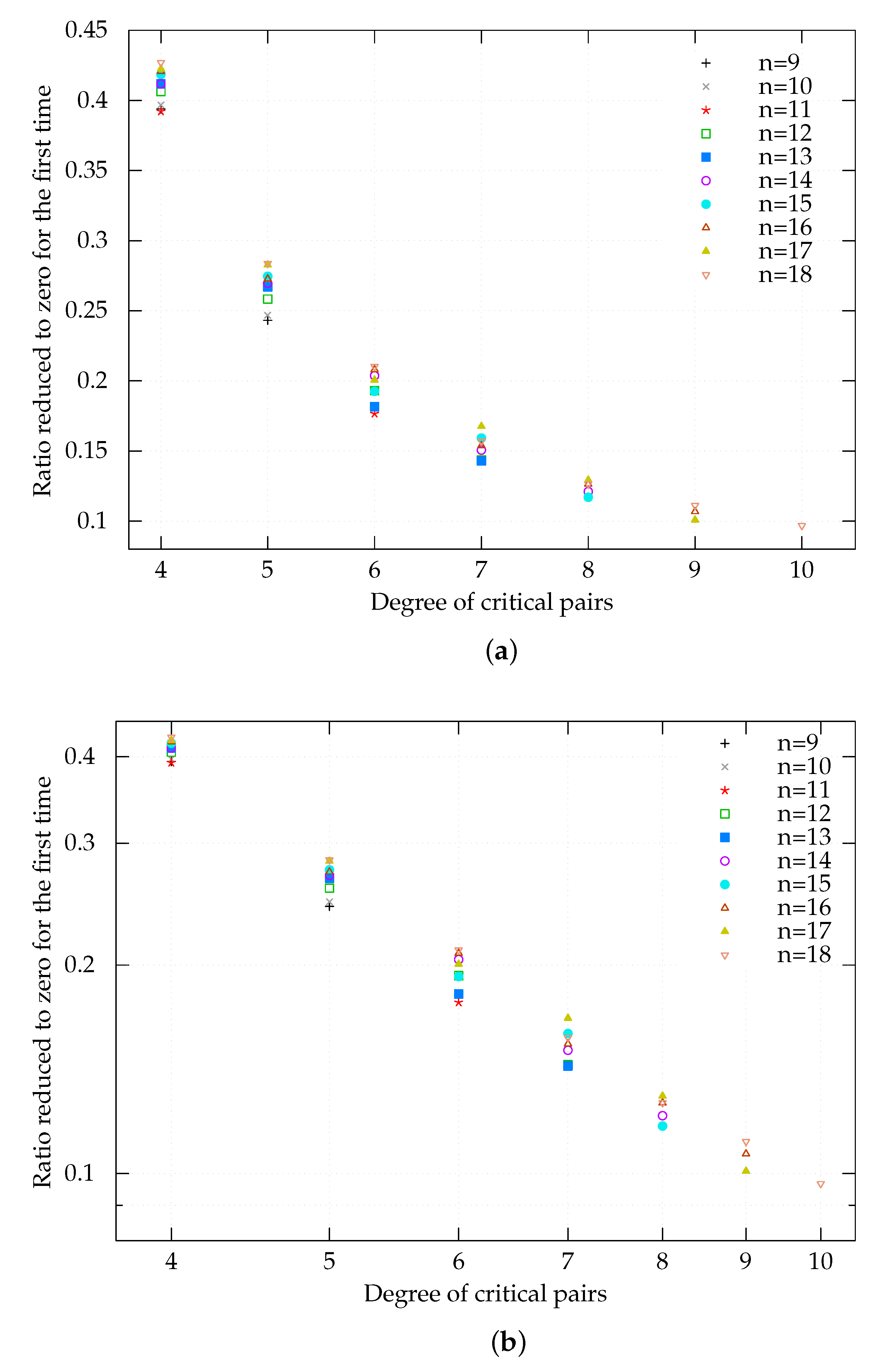
Herein, the computation until the degree of the selected pair becomes $D_{\max }$ is referred to as the first half. In the first half of the computation, many redundant pairs are reduced to zero. When solving the MQ problem, Ito et al. found that if a critical pair of degree d is reduced to zero, all pairs of degree d stored at that time are also reduced to zero with a high probability. Thus, redundant critical pairs can be efficiently eliminated by ignoring all stored pairs of degree d after the critical pairs of degree d are reduced to zero. Algorithm 7 introduces the above method into Algorithm 3. In Algorithm 7, $P_d$ is the set of pairs with the lowest degree d that are not tested. The subset $P^{\prime }$ contains critical pairs selected from $P_d$, and $H^{+}$ refers to new polynomials obtained by reducing $P^{\prime }$. If the number of new polynomials $H^{+}$ is less than the number of selected pairs $P^{\prime }$, a reduction to zero has occurred, and then $P_d$ is deleted.

Algorithm 7 F4-style algorithm proposed by Ito et al.

Input:$F=\{f_1,\dots ,f_m\}\subset \mathcal{R}$. Output: A Gröbner basis of $\langle F\rangle$. 1: $(G,P)\leftarrow (\varnothing ,\varnothing ),i\leftarrow 0,D_{\max }\leftarrow 0$ 2: for$f\in F$do 3:     $(G,P)\leftarrow$ Update $(G,P,f)$ 4: end for 5: while$P\ne \varnothing$do 6:     $(P_d,d)\leftarrow$ Select $\left(P\right)$ 7:     if $D_{\max }<d$ then 8:         $D_{\max }\leftarrow d$ 9:     end if 10:     while $P_d\ne \varnothing$ do 11:         $i\leftarrow i+1$ 12:         $P^{\prime }\leftarrow$ a subset of $P_d$ 13:         $(P,P_d)\leftarrow (P\backslash P^{\prime },P_d\backslash P^{\prime })$ 14:         $L\leftarrow \{\mathrm{Left}\left(p\right)\mid p\in P^{\prime }\}\cup \{\mathrm{Right}\left(p\right)\mid p\in P^{\prime }\}$ 15:         $({\widetilde{H_i}}^{+},H_i)\leftarrow \mathrm{Reduction}(L,G,{\left(H_j\right)}_{j=1,\dots ,i-1})$ 16:         for $h\in {\widetilde{H_i}}^{+}\backslash \left\{0\right\}$ do 17:            $(G,P)\leftarrow$ Update $(G,P,h)$ 18:         end for 19:         if ${}^{\exists }h\in {\widetilde{H_i}}^{+}\backslash \left\{0\right\}$ s.t. $deg\left(h\right)<d$ then 20:            break 21:         end if 22:         if $|{\widetilde{H_i}}^{+}|<|P^{\prime }|$ and $D_{\max }=d$ then 23:            $(P,P_d)\leftarrow (P\backslash P_d,\varnothing )$ 24:         end if 25:     end while 26: end while 27: returnG

Note that Ito et al. stated that the proposed method was valid for MQ problems associated with encryption schemes, i.e., of type $m=2n$, but other MQ problems, including those of type $m=n+1$, were not discussed. Moreover, they set the number of selected pairs $|P^{\prime }|$ to 256 to divide $P_d$. Hence, they did not guarantee that this subdividing method is optimal.

3.4. Proposed Methods

We explain the subdividing methods and the removal method in Section 3.4.1 and Section 3.4.2, respectively. The proposed methods were integrated into the F4-style algorithm as described in Algorithm 8. The OpenF4 library was used for these implementations. The OpenF4 library is an open-source implementation of the F4-style algorithm and, thus, is suitable for this purpose.

Algorithm 8 F4-style algorithm integrating the proposed methods

Input:$F=\{f_1,\dots ,f_m\}\subset \mathcal{R}$. Output: A basis of $\langle F\rangle$. 1: $(G,P)\leftarrow (\varnothing ,\varnothing ),i\leftarrow 0$ 2: for$h\in F$do 3:     $(G,P)\leftarrow$ Update $(G,P,h)$ 4: end for 5: while$P\ne \varnothing$  do 6:     $(P_d,d)\leftarrow$ Select $\left(P\right)$ 7:     $P\leftarrow P\backslash P_d$ 8:     while $P_d\ne \varnothing$ do 9:         // Use the method presented in Section 3.4.1 10:         $\{C_1,\dots ,C_k\}\leftarrow$ SubDividePd $\left(P_d\right)$ 11:         for $l=1\mathbf{to}k$ do 12:            $i\leftarrow i+1$ 13:            $P_d\leftarrow P_d\backslash C_l$ 14:            $L\leftarrow \{\mathrm{Left}\left(p^{\prime }\right)\mid p^{\prime }\in C_l\}\cup \{\mathrm{Right}\left(p^{\prime }\right)\mid p^{\prime }\in C_l\}$ 15:            $({\widetilde{H_i}}^{+},H_i)\leftarrow \mathrm{Reduction}(L,G,{\left(H_j\right)}_{j=1,\dots ,i-1})$ 16:            for $h\in {\widetilde{H_i}}^{+}\backslash \left\{0\right\}$ do 17:                $(G,P)\leftarrow$ Update $(G,P,h)$ 18:            end for 19:            // Use the method presented in Section 3.4.2 20:            if $0\in {\widetilde{H_i}}^{+}$ then 21:                $P_d\leftarrow \varnothing$ 22:                break 23:            end if 24:         end for 25:     end while 26: end while 27: returnG

Algorithm 9 SubDividePd

Input:$P_d\subset P$ and $d\in \mathbb{N}$. Output: $C_1,\dots ,C_k\subset P_d$ 1: $P_d=C_1\bigsqcup C_2\bigsqcup \cdots \bigsqcup C_k$ (disjoint union) s.t. $C_i\prec C_j$ for $i<j$ 2: return$\{C_1,\dots ,C_k\}$

As mentioned above, the SelectPd function serves to select a subset $P_d$ of all the critical pairs at each step for the reduction part of the F4-style algorithm. Ito et al. proposed a method where they subdivide $P_d$ into smaller subsets $\{C_1,\dots ,C_k\}$ as described in Algorithm 9, and perform the Reduction and Update functions for each set $C_i$ consecutively when no S-polynomials are reduced to zero during the reduction. On the other hand, if some S-polynomials reduce to zero during the reduction of a set $C_j$ for the first time, this method ignores the remaining sets $\{C_{j+1},\dots ,C_k\}$ and removes them from all the critical pairs.

The authors confirmed that their method was effective in solving the MQ problems under the condition where $m=2n$ and $k=256$ only and they did not mention other types, especially $m=n+1$, or other subdividing methods.

In our experiments, as described in Section 4.1, we generated the MQ problems ($m=n+1$) with random polynomial coefficients to have at least one solution in the same manner as the Fukuoka MQ challenges ([40], Algorithm 2 and Step 4 of Algorithm 1), and we assumed that $\mathrm{LC}\left(f_j\right)\ne 0$ for all input polynomials $f_j$$(j=1,\dots ,m)$ because such polynomials are obtained with non-negligible probability for experimental purposes. Taking a change in variables into account, the probability is exactly $1-{\{1-{(1-1/q)}^m\}}^n$. For example, it is close to 1 for $q=31$ and $(n,m)=(16,17)$.

3.4.1. Subdividing Methods

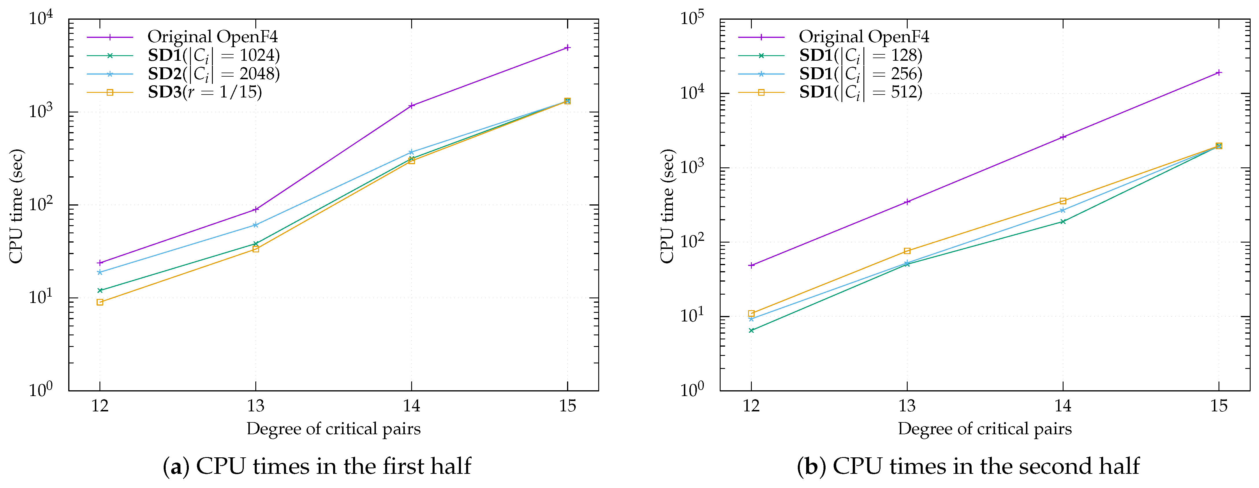
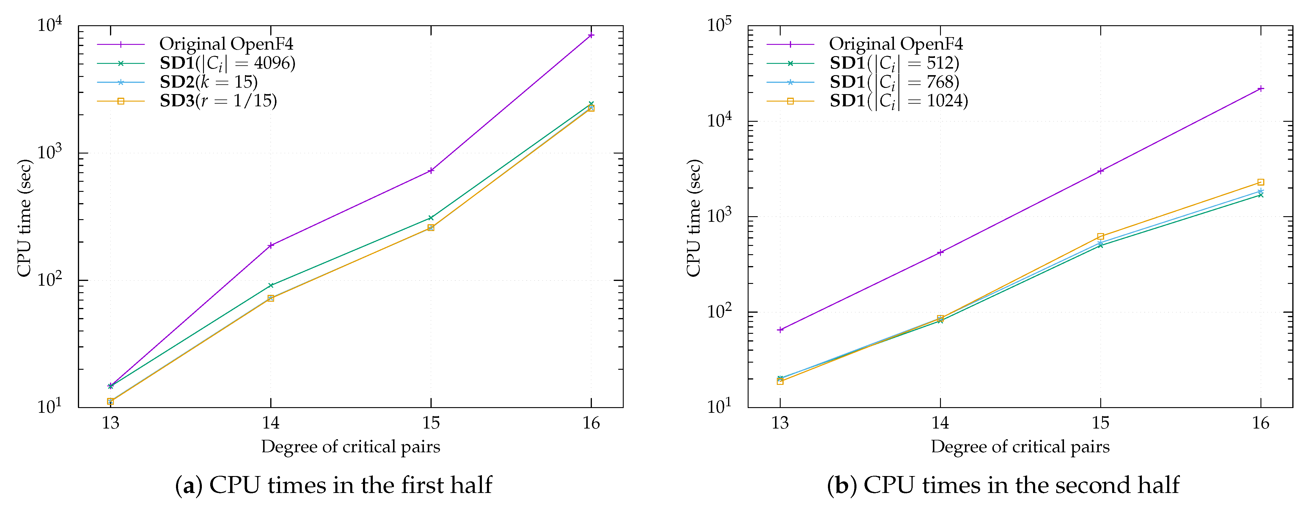
To solve the MQ problems, Ito et al. fixed the number of elements of each $C_i$ to 256, i.e., $|C_i|=256$. In our experiments, we propose three types of subdividing methods:

SD1: 

The number of elements in $C_i$ ($i<k$) is fixed except $C_k$.

We set $|C_i|=128$, 256, 512, 768, 1024, 2048, and 4096.

SD2: 

The number of subdivided subsets is fixed.

We set $k=5$, 10, and 15.

SD3: 

The fraction of elements to be processed in the remaining element in $P_d$ is fixed; i.e., $\mid C_1\mid =max(\lfloor r\mid P_d\mid \rfloor ,1)$ and $\mid C_i\mid =max(\lfloor r\mid P_d\backslash {\cup }_{l=1}^{i-1}{C}_l\mid \rfloor ,1)$ for $i>1$.

We set $r=1/5$, $1/10$, and $1/15$.

Furthermore, we propose two subdividing methods based on SD1 in Section 4.2.

3.4.2. A Removal Method

It is important to skip redundant critical pairs in the $F4$-style algorithm because it takes extra time to compute reductions of larger matrix sizes. To solve the MQ problems that are defined as systems of m quadratic polynomial equations over n variables, Ito et al. experimentally confirmed that once a reduction to zero occurs for some critical pairs in $P^{\prime }\subset P$, nothing but a reduction to zero will be generated for all subsequently selected critical pairs in P in the case of $\mathcal{R}={\mathbb{F}}_{256}$ or ${\mathbb{F}}_{31}$ with the number of polynomials $m=2n$ and the number of variables $n=16,\dots ,25$.

We checked Hypothesis 1 through computational experiments.

Hypothesis 1.

If a Macaulay matrix composed of critical pairs $p^{\prime }\in P^{\prime }$$(\subset P)$ has some reductions to zero, i.e., $0\in \tilde{H}$ in line 15 in Algorithm 8 with the normal strategy, then all remaining critical pairs $p\in P$ s.t. $deg\left(\mathrm{LCM}\left(p\right)\right)=deg\left(\mathrm{LCM}\left(p^{\prime }\right)\right)$ will be reduced to zero with a high probability.

The difference between a measuring algorithm and a checking algorithm is as follows: in the algorithm measuring the software performance of the OpenF4 library and our methods, as defined in Algorithm 8, once a reduction to zero occurs, the remaining critical pairs in $P_d$ are removed. In other words, in such an algorithm, a new next $P_d$ is selected immediately after a reduction to zero. On the other hand, in the algorithm checking Hypothesis 1 as described above, we need to continue reducing all remaining critical pairs and monitor whether reductions to zero are consecutively generated after the first one. However, because the behavior of the checking algorithm needs to match that of the measuring one, every internal state just before processing the remaining critical pairs in the checking algorithm is reset to the state immediately after a reduction to zero.

To check Hypothesis 1, we solved the MQ problems of random coefficients over ${\mathbb{F}}_{31}$ for the condition where $m=n+1$ and $n=9,\dots ,16$ using Algorithm 8 with SD1. Due to processing times, a hundred samples and fifty samples were generated for each problem for $n<16$ and $n=16$, respectively. Furthermore, $\mid C_i\mid$ of SD1 was fixed to 1, 16, 32, 256, and 512 for $n=9,\dots ,12$; $n=13$; $n=14$; $n=15$; and $n=16$, respectively.

Our programs were terminated normally with about $0.9$ probability. Thus, the experiments showed that Hypothesis 1 was valid with about $0.9$ probability. The remaining events, which coincided with a probability of approximately 0.1, corresponded to an OpenF4 library’s warning concerning the number of temporary basis. Although the warning was output, neither temporary basis (i.e., an element in G, in line 17 of Algorithm 8) nor a critical pair of higher degree arose from unused critical pairs in omitted subsets. Moreover, all outputs of all problems contained the initial values with no errors.

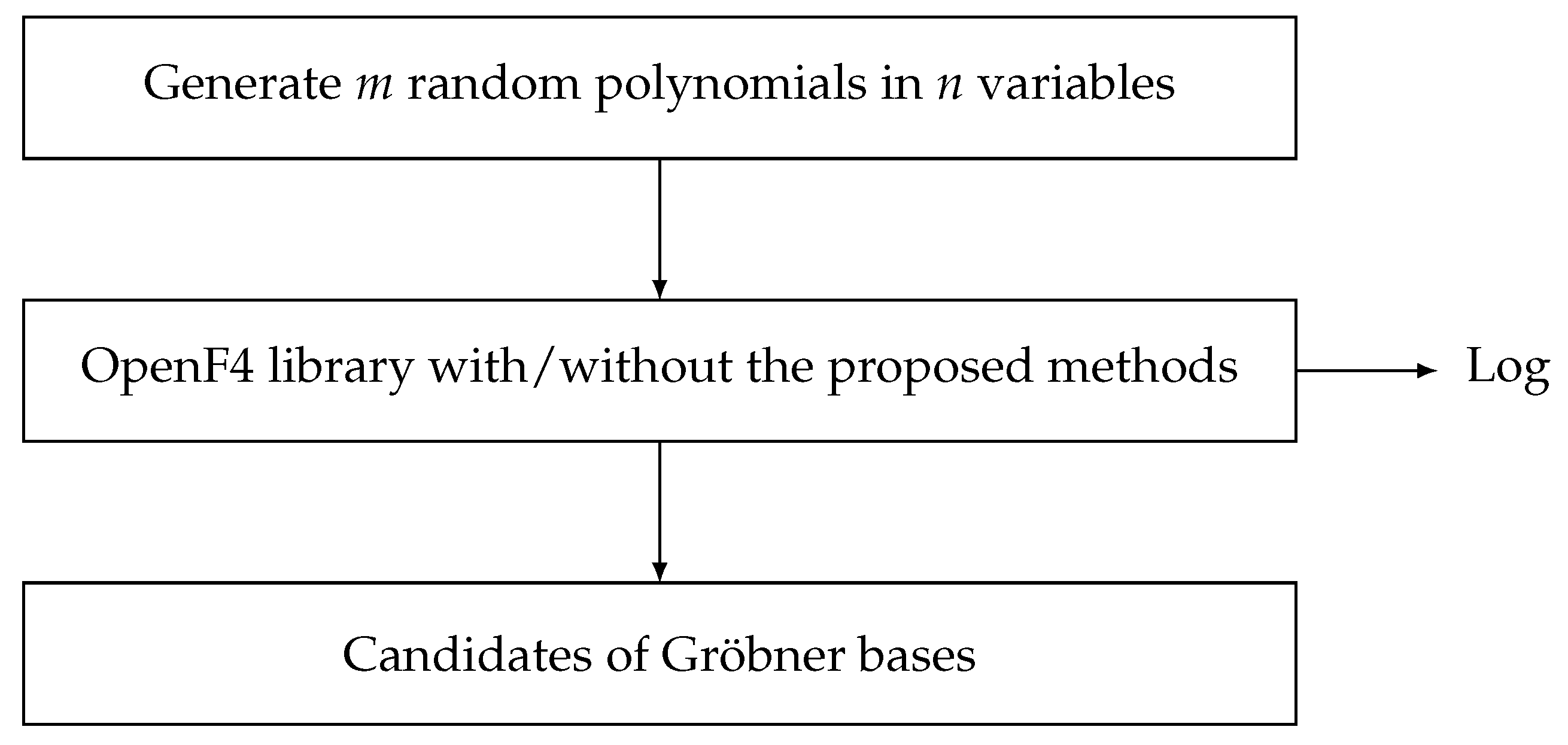
3.5. System Architecture

Our experiments were performed on the following systems as shown in

Table 3. Benchmarking system architecture.

CPU	Intel(R) Xeon(R) Platinum 8180
Clock	2.50 GHz
RAM	1 TB (Non-Uniform Memory Access, NUMA)
Operating System	CentOS 7.9
OpenF4 version	1.0.1, F4::NB_THREAD=1
gcc	4.8.5
compile option	-std=c++11 -O3 -msse4.2 -funroll-loops -ftree-vectorize

and

Table 4. System architecture for computing a reduction to zero.

CPU	Intel(R) Xeon(R) Gold 6254
Clock	3.10 GHz
RAM	3 TB (NUMA)
Operating System	Ubuntu 18.04.01
OpenF4 version	1.0.1, F4::NB_THREAD=1
gcc	7.5.0
compile option	-std=c++11 -O3 -msse4.2 -funroll-loops -ftree-vectorize

. In the case of $(n,m)=(17,18)$ and $(18,19)$ in Appendix A1, our experiments were performed as shown in Table 4.

Our software diagram was as shown in Figure 1.

4. Results

In this section, we describe the software performance of the proposed methods introduced in Section 3.4. Then, we describe their behavior in the first half of the computation.

4.1. Software Performance Comparisons

We integrated our proposed methods into the F4-style algorithm using the OpenF4 library version 1.0.1 and compared their software performances, including the original OpenF4. We benchmarked these implementations on the MQ problems similar to the Fukuoka MQ challenge of type V over a base field ${\mathbb{F}}_{256}$ and type VI over a base field ${\mathbb{F}}_{31}$. These problems were defined as MQ polynomial systems of m equations over n variables with $m=n+1$, based on the hybrid approach. We experimented with ten samples for each parameter: $m=n+1$ and $n=9,\dots ,15$ over ${\mathbb{F}}_{256}$ and $m=n+1$ and $n=9,\dots ,16$ over ${\mathbb{F}}_{31}$. Note that we could not run these programs for $n>16$ over ${\mathbb{F}}_{31}$ and for $n>15$ over ${\mathbb{F}}_{256}$ because the OpenF4 library needs significantly more memory than the RAM installed on our machine. Our results for $m=n+1$ and $n=9,\dots ,15$ over ${\mathbb{F}}_{256}$ are listed in

Table A2. Benchmark results for MQ problems over ${\mathbb{F}}_{256}$ for $m=n+1$, total CPU time (s).

$(\mathit{n},\mathit{m})$	$(9,10)$	$(10,11)$	$(11,12)$	$(12,13)$	$(13,14)$	$(14,15)$	$(15,16)$
Original OpenF4
Average	$2.33\times {10}^{-1}$	$1.58\times {10}^0$	$9.33\times {10}^0$	$7.24\times {10}^1$	$4.38\times {10}^2$	$3.76\times {10}^3$	$2.40\times {10}^4$
$\sigma$	$9.17\times {10}^{-3}$	$2.32\times {10}^{-3}$	$5.25\times {10}^{-3}$	$1.10\times {10}^{-1}$	$2.81\times {10}^{-1}$	$9.77\times {10}^0$	$5.25\times {10}^2$
Before $D_{\max }$	$5.04\times {10}^{-2}$	$5.47\times {10}^{-1}$	$2.00\times {10}^0$	$2.38\times {10}^1$	$8.95\times {10}^1$	$1.17\times {10}^3$	$4.93\times {10}^3$
After $D_{\max }$	$1.80\times {10}^{-1}$	$1.03\times {10}^0$	$7.33\times {10}^0$	$4.86\times {10}^1$	$3.48\times {10}^2$	$2.59\times {10}^3$	$1.91\times {10}^4$
SD1
$\mid C_i\mid =128$ Average	$1.15\times {10}^{-1}$	$5.74\times {10}^{-1}$	$2.90\times {10}^0$	$1.54\times {10}^1$	$8.49\times {10}^1$	$5.72\times {10}^2$	$3.68\times {10}^3$
$\sigma$	$9.80\times {10}^{-4}$	$1.37\times {10}^{-3}$	$4.09\times {10}^{-3}$	$1.74\times {10}^{-2}$	$5.40\times {10}^{-2}$	$5.51\times {10}^{-1}$	$3.00\times {10}^1$
Before $D_{\max }$	$3.32\times {10}^{-2}$	$2.82\times {10}^{-1}$	$9.22\times {10}^{-1}$	$8.91\times {10}^0$	$3.44\times {10}^1$	$3.82\times {10}^2$	$1.73\times {10}^3$
After $D_{\max }$	$7.77\times {10}^{-2}$	$2.85\times {10}^{-1}$	$1.96\times {10}^0$	$6.49\times {10}^0$	$5.04\times {10}^1$	$1.89\times {10}^2$	$1.96\times {10}^3$
$\mid C_i\mid =256$ Average	$1.63\times {10}^{-1}$	$6.50\times {10}^{-1}$	$3.05\times {10}^0$	$1.75\times {10}^1$	$8.62\times {10}^1$	$5.85\times {10}^2$	$3.41\times {10}^3$
$\sigma$	$3.53\times {10}^{-3}$	$9.17\times {10}^{-4}$	$2.42\times {10}^{-3}$	$1.41\times {10}^{-1}$	$5.02\times {10}^{-2}$	$8.31\times {10}^{-1}$	$1.44\times {10}^1$
Before $D_{\max }$	$4.94\times {10}^{-2}$	$3.01\times {10}^{-1}$	$8.80\times {10}^{-1}$	$8.22\times {10}^0$	$3.36\times {10}^1$	$3.15\times {10}^2$	$1.46\times {10}^3$
After $D_{\max }$	$1.10\times {10}^{-1}$	$3.45\times {10}^{-1}$	$2.16\times {10}^0$	$9.30\times {10}^0$	$5.26\times {10}^1$	$2.70\times {10}^2$	$1.95\times {10}^3$
$\mid C_i\mid =512$ Average	$2.18\times {10}^{-1}$	$9.51\times {10}^{-1}$	$4.03\times {10}^0$	$1.89\times {10}^1$	$1.11\times {10}^2$	$6.64\times {10}^2$	$3.33\times {10}^3$
$\sigma$	$7.43\times {10}^{-3}$	$1.86\times {10}^{-3}$	$4.50\times {10}^{-3}$	$8.20\times {10}^{-2}$	$3.60\times {10}^{-2}$	$8.27\times {10}^{-1}$	$1.40\times {10}^1$
Before $D_{\max }$	$4.99\times {10}^{-2}$	$4.41\times {10}^{-1}$	$1.28\times {10}^0$	$7.91\times {10}^0$	$3.46\times {10}^1$	$3.06\times {10}^2$	$1.36\times {10}^3$
After $D_{\max }$	$1.65\times {10}^{-1}$	$5.05\times {10}^{-1}$	$2.74\times {10}^0$	$1.10\times {10}^1$	$7.62\times {10}^1$	$3.58\times {10}^2$	$1.97\times {10}^3$
$\mid C_i\mid =768$ Average	$2.27\times {10}^{-1}$	$1.22\times {10}^0$	$5.11\times {10}^0$	$2.28\times {10}^1$	$1.14\times {10}^2$	$7.10\times {10}^2$	$3.76\times {10}^3$
$\sigma$	$7.76\times {10}^{-3}$	$1.50\times {10}^{-3}$	$3.58\times {10}^{-3}$	$1.24\times {10}^{-2}$	$3.92\times {10}^{-2}$	$1.01\times {10}^0$	$7.57\times {10}^0$
Before $D_{\max }$	$4.97\times {10}^{-2}$	$5.43\times {10}^{-1}$	$1.59\times {10}^0$	$1.00\times {10}^1$	$3.33\times {10}^1$	$3.05\times {10}^2$	$1.33\times {10}^3$
After $D_{\max }$	$1.75\times {10}^{-1}$	$6.70\times {10}^{-1}$	$3.51\times {10}^0$	$1.28\times {10}^1$	$8.07\times {10}^1$	$4.05\times {10}^2$	$2.42\times {10}^3$
$\mid C_i\mid =1024$ Average	$2.29\times {10}^{-1}$	$1.40\times {10}^0$	$6.18\times {10}^0$	$2.68\times {10}^1$	$1.24\times {10}^2$	$7.17\times {10}^2$	$4.40\times {10}^3$
$\sigma$	$8.80\times {10}^{-3}$	$3.53\times {10}^{-3}$	$2.80\times {10}^{-3}$	$4.58\times {10}^{-2}$	$3.18\times {10}^{-1}$	$4.52\times {10}^{-1}$	$1.35\times {10}^1$
Before $D_{\max }$	$4.95\times {10}^{-2}$	$5.44\times {10}^{-1}$	$1.93\times {10}^0$	$1.20\times {10}^1$	$3.84\times {10}^1$	$3.16\times {10}^2$	$1.32\times {10}^3$
After $D_{\max }$	$1.77\times {10}^{-1}$	$8.50\times {10}^{-1}$	$4.25\times {10}^0$	$1.47\times {10}^1$	$8.58\times {10}^1$	$4.01\times {10}^2$	$3.07\times {10}^3$
$\mid C_i\mid =2048$ Average	$2.30\times {10}^{-1}$	$1.57\times {10}^0$	$8.63\times {10}^0$	$4.17\times {10}^1$	$1.85\times {10}^2$	$9.04\times {10}^2$	$4.91\times {10}^3$
$\sigma$	$9.07\times {10}^{-3}$	$1.19\times {10}^{-3}$	$5.04\times {10}^{-2}$	$2.42\times {10}^{-2}$	$3.00\times {10}^{-1}$	$1.80\times {10}^0$	$9.34\times {10}^0$
Before $D_{\max }$	$4.98\times {10}^{-2}$	$5.42\times {10}^{-1}$	$1.99\times {10}^0$	$1.89\times {10}^1$	$6.11\times {10}^1$	$3.71\times {10}^2$	$1.31\times {10}^3$
After $D_{\max }$	$1.77\times {10}^{-1}$	$1.03\times {10}^0$	$6.64\times {10}^0$	$2.28\times {10}^1$	$1.23\times {10}^2$	$5.33\times {10}^2$	$3.60\times {10}^3$
$\mid C_i\mid =4096$  Average	$2.30\times {10}^{-1}$	$1.57\times {10}^0$	$9.35\times {10}^0$	$6.35\times {10}^1$	$2.92\times {10}^2$	$1.34\times {10}^3$	$6.47\times {10}^3$
$\sigma$	$9.19\times {10}^{-3}$	$6.40\times {10}^{-4}$	$8.52\times {10}^{-2}$	$1.12\times {10}^{-2}$	$2.14\times {10}^{-1}$	$5.00\times {10}^{-1}$	$1.73\times {10}^1$
Before $D_{\max }$	$4.95\times {10}^{-2}$	$5.43\times {10}^{-1}$	$1.99\times {10}^0$	$2.37\times {10}^1$	$8.93\times {10}^1$	$5.80\times {10}^2$	$1.99\times {10}^3$
After $D_{\max }$	$1.77\times {10}^{-1}$	$1.03\times {10}^0$	$7.36\times {10}^0$	$3.97\times {10}^1$	$2.03\times {10}^2$	$7.57\times {10}^2$	$4.49\times {10}^3$
SD2
$k=5$         Average	$1.17\times {10}^{-1}$	$5.86\times {10}^{-1}$	$3.33\times {10}^0$	$2.21\times {10}^1$	$1.38\times {10}^2$	$1.09\times {10}^3$	$7.25\times {10}^3$
$\sigma$	$1.14\times {10}^{-2}$	$1.02\times {10}^{-3}$	$2.54\times {10}^{-2}$	$9.39\times {10}^{-3}$	$1.68\times {10}^{-1}$	$9.22\times {10}^{-1}$	$5.91\times {10}^1$
Before $D_{\max }$	$3.50\times {10}^{-2}$	$2.35\times {10}^{-1}$	$8.18\times {10}^{-1}$	$7.38\times {10}^0$	$3.02\times {10}^1$	$3.41\times {10}^2$	$1.48\times {10}^3$
After $D_{\max }$	$6.59\times {10}^{-2}$	$3.41\times {10}^{-1}$	$2.50\times {10}^0$	$1.47\times {10}^1$	$1.08\times {10}^2$	$7.50\times {10}^2$	$5.77\times {10}^3$
$k=10$   Average	$1.27\times {10}^{-1}$	$5.38\times {10}^{-1}$	$2.67\times {10}^0$	$1.89\times {10}^1$	$9.63\times {10}^1$	$8.69\times {10}^2$	$5.58\times {10}^3$
$\sigma$	$4.58\times {10}^{-4}$	$7.81\times {10}^{-4}$	$2.51\times {10}^{-2}$	$1.00\times {10}^{-2}$	$3.96\times {10}^{-2}$	$1.22\times {10}^0$	$1.03\times {10}^1$
Before $D_{\max }$	$3.64\times {10}^{-2}$	$2.63\times {10}^{-1}$	$9.39\times {10}^{-1}$	$8.02\times {10}^0$	$3.19\times {10}^1$	$3.40\times {10}^2$	$1.49\times {10}^3$
After $D_{\max }$	$4.74\times {10}^{-2}$	$2.61\times {10}^{-1}$	$1.71\times {10}^0$	$1.08\times {10}^1$	$6.44\times {10}^1$	$5.30\times {10}^2$	$4.10\times {10}^3$
$k=15$   Average	$1.19\times {10}^{-1}$	$5.23\times {10}^{-1}$	$2.73\times {10}^0$	$1.66\times {10}^1$	$9.53\times {10}^1$	$7.47\times {10}^2$	$3.77\times {10}^3$
$\sigma$	$3.00\times {10}^{-4}$	$1.11\times {10}^{-3}$	$3.87\times {10}^{-3}$	$8.85\times {10}^{-3}$	$1.19\times {10}^{-1}$	$9.83\times {10}^{-1}$	$8.57\times {10}^0$
Before $D_{\max }$	$3.73\times {10}^{-2}$	$2.71\times {10}^{-1}$	$1.06\times {10}^0$	$8.64\times {10}^0$	$3.41\times {10}^1$	$3.08\times {10}^2$	$1.33\times {10}^3$
After $D_{\max }$	$4.60\times {10}^{-2}$	$2.25\times {10}^{-1}$	$1.62\times {10}^0$	$7.85\times {10}^0$	$6.06\times {10}^1$	$4.39\times {10}^2$	$2.44\times {10}^3$
SD3
$r=1/5$      Average	$1.12\times {10}^{-1}$	$5.81\times {10}^{-1}$	$3.27\times {10}^0$	$2.21\times {10}^1$	$1.35\times {10}^2$	$1.09\times {10}^3$	$7.04\times {10}^3$
$\sigma$	$1.02\times {10}^{-3}$	$8.72\times {10}^{-4}$	$4.84\times {10}^{-3}$	$6.02\times {10}^{-3}$	$7.38\times {10}^{-2}$	$6.49\times {10}^{-1}$	$8.54\times {10}^1$
Before $D_{\max }$	$3.49\times {10}^{-2}$	$2.28\times {10}^{-1}$	$8.06\times {10}^{-1}$	$7.35\times {10}^0$	$3.00\times {10}^1$	$3.40\times {10}^2$	$1.48\times {10}^3$
After $D_{\max }$	$6.79\times {10}^{-2}$	$3.40\times {10}^{-1}$	$2.44\times {10}^0$	$1.47\times {10}^1$	$1.05\times {10}^2$	$7.50\times {10}^2$	$5.56\times {10}^3$
$r=1/10$   Average	$1.16\times {10}^{-1}$	$5.36\times {10}^{-1}$	$2.96\times {10}^0$	$1.92\times {10}^1$	$1.15\times {10}^2$	$8.60\times {10}^2$	$5.88\times {10}^3$
$\sigma$	$5.39\times {10}^{-4}$	$4.90\times {10}^{-4}$	$2.23\times {10}^{-3}$	$7.58\times {10}^{-3}$	$4.53\times {10}^{-2}$	$1.09\times {10}^0$	$4.79\times {10}^1$
Before $D_{\max }$	$3.60\times {10}^{-2}$	$2.60\times {10}^{-1}$	$9.19\times {10}^{-1}$	$8.37\times {10}^0$	$3.14\times {10}^1$	$3.30\times {10}^2$	$1.47\times {10}^3$
After $D_{\max }$	$6.58\times {10}^{-2}$	$2.62\times {10}^{-1}$	$2.02\times {10}^{-0}$	$1.08\times {10}^1$	$8.34\times {10}^1$	$5.30\times {10}^2$	$4.41\times {10}^3$
$r=1/15$   Average	$1.17\times {10}^{-1}$	$5.55\times {10}^{-1}$	$3.19\times {10}^0$	$1.66\times {10}^1$	$9.41\times {10}^1$	$7.44\times {10}^2$	$4.94\times {10}^3$
$\sigma$	$3.00\times {10}^{-4}$	$7.00\times {10}^{-4}$	$2.88\times {10}^{-3}$	$1.19\times {10}^{-1}$	$1.12\times {10}^{-1}$	$1.07\times {10}^0$	$9.59\times {10}^0$
Before $D_{\max }$	$4.26\times {10}^{-2}$	$2.87\times {10}^{-1}$	$1.04\times {10}^0$	$8.99\times {10}^0$	$3.35\times {10}^1$	$2.98\times {10}^2$	$1.31\times {10}^3$
After $D_{\max }$	$5.45\times {10}^{-2}$	$2.48\times {10}^{-1}$	$2.12\times {10}^0$	$7.55\times {10}^0$	$6.05\times {10}^1$	$4.46\times {10}^2$	$3.63\times {10}^3$
SD3 followed by SD1 with $r=1/15$ and $\mid C_i\mid =512$
Average	$2.23\times {10}^{-1}$	$8.20\times {10}^{-1}$	$3.78\times {10}^0$	$2.01\times {10}^1$	$1.11\times {10}^2$	$6.53\times {10}^2$	$3.24\times {10}^3$
$\sigma$	$6.45\times {10}^{-3}$	$9.00\times {10}^{-4}$	$3.04\times {10}^{-3}$	$1.33\times {10}^{-2}$	$9.05\times {10}^{-2}$	$5.78\times {10}^{-1}$	$1.35\times {10}^1$
Before $D_{\max }$	$4.28\times {10}^{-2}$	$2.89\times {10}^{-1}$	$1.05\times {10}^0$	$9.00\times {10}^0$	$3.36\times {10}^1$	$2.96\times {10}^2$	$1.30\times {10}^3$
After $D_{\max }$	$1.65\times {10}^{-1}$	$5.13\times {10}^{-1}$	$2.71\times {10}^0$	$1.11\times {10}^1$	$7.69\times {10}^1$	$3.57\times {10}^2$	$1.94\times {10}^3$
SD4 followed by SD1 with $\mid C_i\mid =512$
Average	$1.91\times {10}^{-1}$	$7.09\times {10}^{-1}$	$3.48\times {10}^0$	$1.75\times {10}^1$	$1.03\times {10}^2$	$6.14\times {10}^2$	$3.10\times {10}^3$
$\sigma$	$6.78\times {10}^{-3}$	$6.00\times {10}^{-4}$	$3.29\times {10}^{-3}$	$1.41\times {10}^{-2}$	$7.21\times {10}^{-2}$	$1.76\times {10}^0$	$1.11\times {10}^1$
Before $D_{\max }$	$2.30\times {10}^{-2}$	$1.96\times {10}^{-1}$	$7.25\times {10}^{-1}$	$6.46\times {10}^0$	$2.61\times {10}^1$	$2.55\times {10}^2$	$1.14\times {10}^3$
After $D_{\max }$	$1.64\times {10}^{-1}$	$5.08\times {10}^{-1}$	$2.74\times {10}^0$	$1.10\times {10}^1$	$7.68\times {10}^1$	$3.59\times {10}^2$	$1.95\times {10}^3$
SD5 followed by SD1 with $\mid C_i\mid =512$
Average	$1.39\times {10}^{-1}$	$6.25\times {10}^{-1}$	$3.33\times {10}^0$	$1.97\times {10}^1$	$1.09\times {10}^2$	$8.09\times {10}^2$	$4.26\times {10}^3$
$\sigma$	$6.64\times {10}^{-3}$	$2.61\times {10}^{-3}$	$1.68\times {10}^{-2}$	$8.88\times {10}^{-3}$	$5.87\times {10}^{-2}$	$9.52\times {10}^{-1}$	$6.62\times {10}^0$
Before $D_{\max }$	$2.49\times {10}^{-2}$	$2.20\times {10}^{-1}$	$7.96\times {10}^{-1}$	$7.44\times {10}^0$	$3.04\times {10}^1$	$3.14\times {10}^2$	$1.42\times {10}^3$
After $D_{\max }$	$1.10\times {10}^{-1}$	$4.00\times {10}^{-1}$	$2.53\times {10}^0$	$1.23\times {10}^1$	$7.83\times {10}^1$	$4.95\times {10}^2$	$2.84\times {10}^3$

σ stands for a standard deviation.

and for $m=n+1$ and $n=9,\dots ,16$ over ${\mathbb{F}}_{31}$ are listed in

Table A3. Benchmark results for MQ problems over ${\mathbb{F}}_{31}$ for $m=n+1$, total CPU time (s).

$(\mathit{n},\mathit{m})$	$(9,10)$	$(10,11)$	$(11,12)$	$(12,13)$	$(13,14)$	$(14,15)$	$(15,16)$	$(16,17)$
Original OpenF4
Average	$1.22\times {10}^{-1}$	$5.89\times {10}^{-1}$	$2.55\times {10}^0$	$1.38\times {10}^1$	$8.00\times {10}^1$	$6.30\times {10}^2$	$3.74\times {10}^3$	$3.04\times {10}^4$
$\sigma$	$2.12\times {10}^{-3}$	$3.44\times {10}^{-3}$	$1.01\times {10}^{-1}$	$1.51\times {10}^0$	$1.78\times {10}^{-1}$	$2.32\times {10}^0$	$2.54\times {10}^2$	$4.32\times {10}^2$
Before $D_{\max }$	$2.82\times {10}^{-2}$	$2.04\times {10}^{-1}$	$5.75\times {10}^{-1}$	$4.39\times {10}^0$	$1.48\times {10}^1$	$1.88\times {10}^2$	$7.28\times {10}^2$	$8.46\times {10}^3$
After $D_{\max }$	$8.98\times {10}^{-2}$	$3.81\times {10}^{-1}$	$1.97\times {10}^0$	$9.40\times {10}^0$	$6.52\times {10}^1$	$4.42\times {10}^2$	$3.01\times {10}^3$	$2.20\times {10}^4$
SD1
$|C_i|=128$   Average	$7.07\times {10}^{-2}$	$3.12\times {10}^{-1}$	$1.38\times {10}^0$	$6.88\times {10}^0$	$3.23\times {10}^1$	$2.01\times {10}^2$	$1.32\times {10}^3$	$1.17\times {10}^4$
$\sigma$	$1.00\times {10}^{-3}$	$1.85\times {10}^{-3}$	$2.41\times {10}^{-2}$	$1.42\times {10}^{-1}$	$2.70\times {10}^{-1}$	$5.46\times {10}^{-1}$	$5.33\times {10}^0$	$6.83\times {10}^1$
Before $D_{\max }$	$2.11\times {10}^{-2}$	$1.55\times {10}^{-1}$	$4.25\times {10}^{-1}$	$3.83\times {10}^0$	$1.34\times {10}^1$	$1.38\times {10}^2$	$6.09\times {10}^2$	$8.69\times {10}^3$
After $D_{\max }$	$4.60\times {10}^{-2}$	$1.51\times {10}^{-1}$	$9.46\times {10}^{-1}$	$3.03\times {10}^0$	$1.89\times {10}^1$	$6.27\times {10}^1$	$7.11\times {10}^2$	$3.02\times {10}^3$
$|C_i|=256$   Average	$9.17\times {10}^{-2}$	$3.03\times {10}^{-1}$	$1.24\times {10}^0$	$6.30\times {10}^0$	$2.79\times {10}^1$	$1.66\times {10}^2$	$9.76\times {10}^2$	$7.81\times {10}^3$
$\sigma$	$9.00\times {10}^{-4}$	$2.42\times {10}^{-3}$	$5.33\times {10}^{-3}$	$1.31\times {10}^{-1}$	$7.61\times {10}^{-2}$	$2.76\times {10}^{-1}$	$1.54\times {10}^0$	$2.45\times {10}^1$
Before $D_{\max }$	$2.73\times {10}^{-2}$	$1.39\times {10}^{-1}$	$3.43\times {10}^{-1}$	$2.79\times {10}^0$	$1.03\times {10}^1$	$9.01\times {10}^1$	$4.02\times {10}^2$	$5.35\times {10}^3$
After $D_{\max }$	$5.93\times {10}^{-2}$	$1.60\times {10}^{-1}$	$8.85\times {10}^{-1}$	$3.50\times {10}^0$	$1.76\times {10}^1$	$7.61\times {10}^1$	$5.74\times {10}^2$	$2.47\times {10}^3$
$|C_i|=512$   Average	$1.12\times {10}^{-1}$	$3.83\times {10}^{-1}$	$1.35\times {10}^0$	$5.52\times {10}^0$	$2.90\times {10}^1$	$1.52\times {10}^2$	$7.97\times {10}^2$	$5.39\times {10}^3$
$\sigma$	$2.09\times {10}^{-3}$	$2.24\times {10}^{-3}$	$2.59\times {10}^{-2}$	$2.65\times {10}^{-1}$	$1.03\times {10}^{-2}$	$1.36\times {10}^{-1}$	$1.98\times {10}^0$	$1.70\times {10}^1$
Before $D_{\max }$	$2.74\times {10}^{-2}$	$1.72\times {10}^{-1}$	$4.30\times {10}^{-1}$	$2.06\times {10}^0$	$8.69\times {10}^0$	$7.10\times {10}^1$	$2.99\times {10}^2$	$3.70\times {10}^3$
After $D_{\max }$	$8.08\times {10}^{-2}$	$2.05\times {10}^{-1}$	$9.12\times {10}^{-1}$	$3.45\times {10}^0$	$2.03\times {10}^1$	$8.12\times {10}^1$	$4.99\times {10}^2$	$1.69\times {10}^3$
$|C_i|=768$   Average	$1.18\times {10}^{-1}$	$4.57\times {10}^{-1}$	$1.56\times {10}^0$	$5.91\times {10}^0$	$2.72\times {10}^1$	$1.52\times {10}^2$	$8.02\times {10}^2$	$5.12\times {10}^3$
$\sigma$	$2.18\times {10}^{-3}$	$1.85\times {10}^{-3}$	$2.20\times {10}^{-2}$	$1.89\times {10}^{-1}$	$9.46\times {10}^{-3}$	$2.13\times {10}^0$	$1.31\times {10}^0$	$5.24\times {10}^1$
Before $D_{\max }$	$2.75\times {10}^{-2}$	$1.99\times {10}^{-1}$	$4.91\times {10}^{-1}$	$2.41\times {10}^0$	$7.07\times {10}^0$	$6.51\times {10}^1$	$2.67\times {10}^2$	$3.25\times {10}^3$
After $D_{\max }$	$8.59\times {10}^{-2}$	$2.53\times {10}^{-1}$	$1.06\times {10}^0$	$3.49\times {10}^0$	$2.01\times {10}^1$	$8.67\times {10}^1$	$5.35\times {10}^2$	$1.86\times {10}^3$
$|C_i|=1024$   Average	$1.19\times {10}^{-1}$	$5.17\times {10}^{-1}$	$1.81\times {10}^0$	$6.70\times {10}^0$	$2.66\times {10}^1$	$1.49\times {10}^2$	$8.68\times {10}^2$	$5.05\times {10}^3$
$\sigma$	$1.80\times {10}^{-3}$	$2.37\times {10}^{-3}$	$1.75\times {10}^{-2}$	$1.40\times {10}^{-1}$	$4.72\times {10}^{-2}$	$1.54\times {10}^0$	$1.77\times {10}^0$	$3.06\times {10}^1$
Before $D_{\max }$	$2.72\times {10}^{-2}$	$2.00\times {10}^{-1}$	$5.60\times {10}^{-1}$	$2.75\times {10}^0$	$7.79\times {10}^0$	$6.28\times {10}^1$	$2.45\times {10}^2$	$2.75\times {10}^3$
After $D_{\max }$	$8.72\times {10}^{-2}$	$3.13\times {10}^{-1}$	$1.24\times {10}^0$	$3.95\times {10}^0$	$1.88\times {10}^1$	$8.61\times {10}^1$	$6.22\times {10}^2$	$2.30\times {10}^3$
$|C_i|=2048$   Average	$1.18\times {10}^{-1}$	$5.79\times {10}^{-1}$	$2.34\times {10}^0$	$8.98\times {10}^0$	$3.42\times {10}^1$	$1.56\times {10}^2$	$8.63\times {10}^2$	$5.20\times {10}^3$
$\sigma$	$1.68\times {10}^{-3}$	$1.83\times {10}^{-3}$	$3.16\times {10}^{-2}$	$1.43\times {10}^{-1}$	$2.05\times {10}^{-2}$	$4.88\times {10}^{-1}$	$1.15\times {10}^1$	$2.37\times {10}^1$
Before $D_{\max }$	$2.73\times {10}^{-2}$	$1.99\times {10}^{-1}$	$5.79\times {10}^{-1}$	$3.71\times {10}^0$	$1.07\times {10}^1$	$6.16\times {10}^1$	$2.14\times {10}^2$	$2.46\times {10}^3$
After $D_{\max }$	$8.66\times {10}^{-2}$	$3.76\times {10}^{-1}$	$1.77\times {10}^0$	$5.26\times {10}^0$	$2.34\times {10}^1$	$9.39\times {10}^1$	$6.48\times {10}^2$	$2.73\times {10}^3$
$|C_i|=4096$ Average	$1.19\times {10}^{-1}$	$5.81\times {10}^{-1}$	$2.54\times {10}^0$	$1.23\times {10}^1$	$5.27\times {10}^1$	$2.16\times {10}^2$	$1.05\times {10}^3$	$6.09\times {10}^3$
$\sigma$	$1.63\times {10}^{-3}$	$2.54\times {10}^{-3}$	$9.76\times {10}^{-2}$	$9.86\times {10}^{-1}$	$1.15\times {10}^{-1}$	$8.77\times {10}^{-1}$	$1.48\times {10}^1$	$4.83\times {10}^1$
Before $D_{\max }$	$2.72\times {10}^{-2}$	$2.00\times {10}^{-1}$	$5.69\times {10}^{-1}$	$4.36\times {10}^0$	$1.47\times {10}^1$	$9.12\times {10}^1$	$3.10\times {10}^2$	$2.44\times {10}^3$
After $D_{\max }$	$8.72\times {10}^{-2}$	$3.76\times {10}^{-1}$	$1.96\times {10}^0$	$7.91\times {10}^0$	$3.80\times {10}^1$	$1.25\times {10}^2$	$7.39\times {10}^2$	$3.65\times {10}^3$
SD2
$k=5$         Average	$7.91\times {10}^{-2}$	$3.01\times {10}^{-1}$	$1.32\times {10}^0$	$6.13\times {10}^0$	$2.88\times {10}^1$	$1.83\times {10}^2$	$1.22\times {10}^3$	$8.53\times {10}^3$
$\sigma$	$2.12\times {10}^{-3}$	$1.99\times {10}^{-3}$	$1.35\times {10}^{-1}$	$3.98\times {10}^{-1}$	$2.44\times {10}^{-2}$	$7.03\times {10}^{-2}$	$5.35\times {10}^2$	$2.30\times {10}^2$
Before $D_{\max }$	$2.64\times {10}^{-2}$	$1.32\times {10}^{-1}$	$3.62\times {10}^{-1}$	$2.07\times {10}^0$	$6.79\times {10}^0$	$5.97\times {10}^1$	$2.22\times {10}^2$	$2.42\times {10}^3$
After $D_{\max }$	$4.51\times {10}^{-1}$	$1.60\times {10}^{-1}$	$9.22\times {10}^{-1}$	$4.03\times {10}^0$	$2.20\times {10}^1$	$1.23\times {10}^2$	$1.00\times {10}^3$	$6.11\times {10}^3$
$k=10$   Average	$1.17\times {10}^{-1}$	$3.38\times {10}^{-1}$	$1.37\times {10}^0$	$6.67\times {10}^0$	$2.67\times {10}^1$	$1.65\times {10}^2$	$9.63\times {10}^2$	$7.10\times {10}^3$
$\sigma$	$1.08\times {10}^{-3}$	$2.05\times {10}^{-3}$	$8.76\times {10}^{-3}$	$1.09\times {10}^0$	$2.97\times {10}^{-1}$	$2.45\times {10}^{-1}$	$9.38\times {10}^{-1}$	$9.41\times {10}^2$
Before $D_{\max }$	$3.16\times {10}^{-2}$	$1.74\times {10}^{-1}$	$4.93\times {10}^{-1}$	$2.89\times {10}^0$	$9.10\times {10}^0$	$7.15\times {10}^1$	$2.74\times {10}^2$	$2.58\times {10}^3$
After $D_{\max }$	$3.94\times {10}^{-2}$	$1.48\times {10}^{-1}$	$8.51\times {10}^{-1}$	$3.72\times {10}^0$	$1.76\times {10}^1$	$9.38\times {10}^1$	$6.89\times {10}^2$	$4.51\times {10}^3$
$k=15$   Average	$1.13\times {10}^{-1}$	$3.68\times {10}^{-1}$	$1.57\times {10}^0$	$7.05\times {10}^0$	$4.29\times {10}^1$	$1.56\times {10}^2$	$8.51\times {10}^2$	$5.73\times {10}^3$
$\sigma$	$8.72\times {10}^{-4}$	$1.55\times {10}^{-3}$	$1.29\times {10}^{-2}$	$5.16\times {10}^{-1}$	$1.03\times {10}^{-1}$	$8.86\times {10}^{-2}$	$1.63\times {10}^0$	$7.39\times {10}^0$
Before $D_{\max }$	$3.41\times {10}^{-2}$	$1.93\times {10}^{-1}$	$6.35\times {10}^{-1}$	$3.64\times {10}^0$	$1.13\times {10}^1$	$7.28\times {10}^1$	$2.58\times {10}^2$	$2.28\times {10}^3$
After $D_{\max }$	$4.03\times {10}^{-2}$	$1.47\times {10}^{-1}$	$8.85\times {10}^{-1}$	$3.32\times {10}^0$	$3.10\times {10}^1$	$8.36\times {10}^1$	$5.92\times {10}^2$	$3.45\times {10}^3$
SD3
$r=1/5$   Average	$8.05\times {10}^{-2}$	$2.99\times {10}^{-1}$	$1.25\times {10}^0$	$5.89\times {10}^0$	$2.81\times {10}^1$	$1.80\times {10}^2$	$1.11\times {10}^3$	$8.39\times {10}^3$
$\sigma$	$1.02\times {10}^{-3}$	$1.61\times {10}^{-3}$	$4.56\times {10}^{-3}$	$4.38\times {10}^{-2}$	$3.32\times {10}^{-2}$	$1.56\times {10}^{-1}$	$5.19\times {10}^1$	$6.57\times {10}^1$
Before $D_{\max }$	$2.54\times {10}^{-2}$	$1.30\times {10}^{-1}$	$3.56\times {10}^{-1}$	$2.03\times {10}^0$	$6.74\times {10}^0$	$5.89\times {10}^1$	$2.39\times {10}^2$	$2.41\times {10}^3$
After $D_{\max }$	$4.41\times {10}^{-2}$	$1.57\times {10}^{-1}$	$8.77\times {10}^{-1}$	$3.84\times {10}^0$	$2.13\times {10}^1$	$1.21\times {10}^2$	$8.75\times {10}^2$	$5.97\times {10}^3$
$r=1/10$      Average	$9.70\times {10}^{-2}$	$3.34\times {10}^{-1}$	$1.44\times {10}^0$	$6.54\times {10}^0$	$2.85\times {10}^1$	$1.63\times {10}^2$	$9.78\times {10}^2$	$6.65\times {10}^3$
$\sigma$	$8.94\times {10}^{-4}$	$1.73\times {10}^{-3}$	$6.32\times {10}^{-3}$	$9.04\times {10}^{-2}$	$1.42\times {10}^{-2}$	$1.84\times {10}^0$	$9.16\times {10}^0$	$5.87\times {10}^1$
Before $D_{\max }$	$3.32\times {10}^{-2}$	$1.73\times {10}^{-1}$	$4.85\times {10}^{-1}$	$3.19\times {10}^0$	$8.94\times {10}^0$	$7.07\times {10}^1$	$2.69\times {10}^2$	$2.52\times {10}^3$
After $D_{\max }$	$5.08\times {10}^{-2}$	$1.44\times {10}^{-1}$	$9.27\times {10}^{-1}$	$3.32\times {10}^0$	$1.96\times {10}^1$	$9.22\times {10}^1$	$7.10\times {10}^2$	$4.13\times {10}^3$
$r=1/15$   Average	$1.08\times {10}^{-1}$	$3.84\times {10}^{-1}$	$1.68\times {10}^0$	$7.02\times {10}^0$	$3.07\times {10}^1$	$1.56\times {10}^2$	$9.08\times {10}^2$	$5.71\times {10}^3$
$\sigma$	$6.00\times {10}^{-4}$	$1.86\times {10}^{-3}$	$7.40\times {10}^{-3}$	$9.72\times {10}^{-2}$	$2.96\times {10}^{-2}$	$2.80\times {10}^{-1}$	$1.67\times {10}^0$	$1.23\times {10}^1$
Before $D_{\max }$	$3.92\times {10}^{-2}$	$2.10\times {10}^{-1}$	$6.33\times {10}^{-1}$	$3.97\times {10}^0$	$1.12\times {10}^1$	$7.22\times {10}^1$	$2.59\times {10}^2$	$2.25\times {10}^3$
After $D_{\max }$	$4.70\times {10}^{-2}$	$1.51\times {10}^{-1}$	$1.02\times {10}^0$	$3.01\times {10}^0$	$1.94\times {10}^1$	$8.39\times {10}^1$	$6.49\times {10}^2$	$3.46\times {10}^3$
SD3+SD1   $r=1/15,|C_i|=512$
Average	$1.36\times {10}^{-1}$	$4.27\times {10}^{-1}$	$1.56\times {10}^0$	$7.22\times {10}^0$	$3.12\times {10}^1$	$1.52\times {10}^2$	$7.52\times {10}^2$	$3.92\times {10}^3$
$\sigma$	$1.08\times {10}^{-3}$	$1.64\times {10}^{-3}$	$2.84\times {10}^{-2}$	$5.30\times {10}^{-2}$	$2.87\times {10}^{-2}$	$9.05\times {10}^{-2}$	$1.10\times {10}^0$	$1.23\times {10}^1$
Before $D_{\max }$	$3.90\times {10}^{-2}$	$2.06\times {10}^{-1}$	$6.19\times {10}^{-1}$	$3.88\times {10}^0$	$1.09\times {10}^1$	$7.04\times {10}^1$	$2.55\times {10}^2$	$2.22\times {10}^3$
After $D_{\max }$	$8.08\times {10}^{-2}$	$2.02\times {10}^{-1}$	$9.11\times {10}^{-1}$	$3.30\times {10}^0$	$2.03\times {10}^1$	$8.10\times {10}^1$	$4.96\times {10}^2$	$1.70\times {10}^3$
SD4+SD1   $|C_i|=512$
Average	$1.03\times {10}^{-1}$	$3.21\times {10}^{-1}$	$1.26\times {10}^0$	$5.38\times {10}^0$	$2.73\times {10}^1$	$1.33\times {10}^2$	$7.11\times {10}^2$	$3.78\times {10}^3$
$\sigma$	$1.02\times {10}^{-3}$	$8.00\times {10}^{-4}$	$6.52\times {10}^{-2}$	$2.76\times {10}^{-1}$	$2.27\times {10}^{-2}$	$1.56\times {10}^{-1}$	$7.46\times {10}^0$	$5.81\times {10}^2$
Before $D_{\max }$	$1.73\times {10}^{-2}$	$1.07\times {10}^{-1}$	$3.20\times {10}^{-1}$	$1.83\times {10}^0$	$6.08\times {10}^0$	$4.89\times {10}^1$	$1.95\times {10}^2$	$2.00\times {10}^3$
After $D_{\max }$	$8.19\times {10}^{-2}$	$2.08\times {10}^{-1}$	$9.38\times {10}^{-1}$	$3.54\times {10}^0$	$2.12\times {10}^1$	$8.43\times {10}^1$	$5.16\times {10}^2$	$1.78\times {10}^3$
SD5+SD1   $|C_i|=512$
Average	$8.34\times {10}^{-2}$	$2.93\times {10}^{-1}$	$1.22\times {10}^0$	$5.69\times {10}^0$	$2.63\times {10}^1$	$1.53\times {10}^2$	$8.09\times {10}^2$	$5.89\times {10}^3$
$\sigma$	$9.14\times {10}^{-4}$	$1.10\times {10}^{-3}$	$2.47\times {10}^{-2}$	$2.03\times {10}^{-1}$	$1.06\times {10}^{-2}$	$2.30\times {10}^{-1}$	$1.34\times {10}^0$	$5.16\times {10}^0$
Before $D_{\max }$	$1.79\times {10}^{-2}$	$1.11\times {10}^{-1}$	$3.20\times {10}^{-1}$	$1.96\times {10}^0$	$6.60\times {10}^0$	$5.49\times {10}^1$	$2.27\times {10}^2$	$2.22\times {10}^3$
After $D_{\max }$	$6.22\times {10}^{-2}$	$1.76\times {10}^{-1}$	$8.95\times {10}^{-1}$	$3.72\times {10}^0$	$1.97\times {10}^1$	$9.83\times {10}^1$	$5.81\times {10}^2$	$3.67\times {10}^3$

σ stands for a standard deviation.

. For the first and second halves of the computation, the top three records produced by the proposed methods and the record by the OpenF4 library are shown in Figure 2a,b and Figure 3a,b.

These experiments demonstrated that there was no failure to compute solutions including initially selected values and standard variations ($\sigma$) of the CPU times were relatively small and the F4-style algorithms integrating our proposed methods were faster than that of the original OpenF4 library, e.g., by a factor of up to $7.21$ in the case of SD1 under $n=15$ and $\mid C_i\mid =512$ over ${\mathbb{F}}_{256}$ and factor $6.02$ in the case of SD1 under $n=16$ and $\mid C_i\mid =1024$ over ${\mathbb{F}}_{31}$. According to these results, we could argue that SD1 is faster than all other methods. However, if we focus only on the first half of the computation, we found that SD3 with $r=15$ may be the fastest in both the cases of ${\mathbb{F}}_{256}$ and ${\mathbb{F}}_{31}$. This reason will be discussed in the next section. If we distinguish between the first and second halves, we conclude that it is appropriate to apply SD3 with $r=15$ in the first half and SD1 with $\mid C_i\mid \le 512$ in the second half. For example, a combination of SD3 with $r=1/15$ for the first half and SD1 with $\mid C_i\mid =512$ for the second half (i.e., SD3 followed by SD1) is faster than otherwise, e.g., by a factor of up to $7.76$ for $(n,m)=(16,17)$ over ${\mathbb{F}}_{31}$.

4.2. The Performance Behavior of the Proposed Methods in the First Half

In our experiments, we calculated the CPU time and the number of critical pairs used at each reduction. We found that the minimum number of critical pairs that generates a reduction to zero for the first time is approximately constant. Note, however, that if more than one of the critical pairs arises, we take the maximum number among them.

The number of critical pairs that generates a reduction to zero for the first time for each $(n,m)$ and d is listed in

Table A1. Experimental results of the minimum number of critical pairs that generates a reduction to zero in the first half for $m=n+1$ over ${\mathbb{F}}_{256}$ and ${\mathbb{F}}_{31}$.

$(\mathit{n},\mathit{m})$		$(9,10)$	$(10,11)$	$(11,12)$	$(12,13)$	$(13,14)$	$(14,15)$	$(15,16)$	$(16,17)$	$(17,18){}^{†}$	$(18,19){}^{†}$
$d=2$	Min	9	10	11	12	13	14	15	16	17	18
	Total	9	10	11	12	13	14	15	16	17	18
$d=3$	Min	20	24	28	32	36	40	45	50	55	60
	Total	20	24	28	32	36	40	45	50	55	60
$d=4$	Min	39	50	60	76	91	106	126	146	165	189
	Total	99	126	153	187	221	256	301	347	393	445
$d=5$	Min	63	88	120	156	204	248	318	378	462	550
	Total	259	354	456	604	764	927	1158	1386	1638	1942
$d=6$	Min	–	132	187	286	364	532	664	901	1089	1424
	Total		737	1059	1432	2004	2612	3449	4331	5443	6780
$d=7$	Min	–	–	–	429	572	936	1300	1768	2448	3078
	Total				3003	4004	6216	8164	11,492	14,616	19,614
$d=8$	Min	–	–	–	–	–	1430	2002	3094	4590	5814
	Total						11,804	17,108	24,480	35,496	45,999
$d=9$	Min	–	–	–	–	–	–	–	4862	7072	10,336
	Total								45,526	70,176	93,024
$d=10$	Min	–	–	–	–	–	–	–	–	–	16,796
	Total										173,774

Min: the minimum number of critical pairs for a reduction to zero. Total: the total number of critical pairs appearing before a reduction. ^† Another NUMA machine that has 3 TB RAM.

. The symbol Total in the table represents the number of critical pairs before reducing the Macaulay matrix for each $(n,m)$ and d. The symbol Min represents the minimum number of critical pairs that generates a reduction to zero for the first time for each $(n,m)$ and d. The ratio of Min-to-Total is shown in Figure 4a. The log-log scale version of this figure is shown in Figure 4b. Figure 4a shows that the ratios gradually decrease, and the decreasing ratios are not constant. These tendencies were likely the reason that SD3 with $r=1/15$ was useful in the first half. Figure 4b shows that it is expected that the errors by the linear approximation will not be so large.

Here, we propose the subdividing method SD4 in the first half as follows.

SD4: 

The number of elements in the first subset $\mid C_1\mid$ is 1 plus the number Min specified in Table A1. $\mid C_i\mid$ $(i>2)$ is fixed to a small value in place.

We experimented with SD4 in the first half followed by SD1 with $\mid C_i\mid =512$ in the second half (i.e., SD4 ⇒ SD1). Our benchmark results of SD4 followed by SD1 are listed in Table A2 and Table A3. For the first half of the computation, the record by SD4 and the record by the OpenF4 library are shown in Figure 5a,b.

Here, we investigate the approximation of the ratio (r) shown in Figure 4a. The Simplify function outputs the product of $x_i\times p$ such that $x_i$ is a variable and p is a polynomial with a high probability, as stated in the paper ([34], Remark 2.6). Thus, it seems likely that the rows of the Macaulay matrix are composed of the products of $x_1^{a_1}\dots x_i^{a_i}\times p$ where $1\le i\le n$ and p is a polynomial with a high probability because of the normal strategy.

Moreover, the elements in the leftmost columns of the Macaulay matrix come from the leading monomials. Hence, it seems reasonable to suppose that the ratio r is approximately related to the number of monomials of degree d:

$$\mid \{x_1^{a_1}\dots x_n^{a_n}|a_1+\cdots +a_n=d\}\mid =\left(\genfrac{}{}{0pt}{}{d+n-1}{n-1}\right)\approx \frac{d^{n-1}}{(n-1)!}+\left(\mathrm{lower}\mathrm{terms}\right).$$

(4)

Accordingly, we assume that r is proportional to a power of d, i.e., $r\propto d^c$ (c is a constant), by ignoring lower terms. We have $logr=alogd+b$ where a and b are constants. Thus, it seems that there is a correspondence between linear approximations of the graphs in Figure 4b and the lower terms on the rightmost side of (4) are ignored. Furthermore, we assume that linear expressions in n approximate both a and b, and we distinguish between the approximations according to whether n is even or odd.

The linear regression analysis of a $(n=9,\dots ,16)$ shows that

$$a\approx a\left(n\right)=\left\{\begin{array}{cc}0.0566n-2.63\hfill & \left(n\mathrm{is}\mathrm{odd}\right),\hfill \\ 0.0443n-2.38\hfill & \left(n\mathrm{is}\mathrm{even}\right).\hfill \end{array}\right.$$

In addition, the regression analysis of b $(n=9,\dots ,16)$ shows that

$$b\approx b\left(n\right)=\left\{\begin{array}{cc}-0.0301n+1.15\hfill & \left(n\mathrm{is}\mathrm{odd}\right),\hfill \\ -0.0236n+1.01\hfill & \left(n\mathrm{is}\mathrm{even}\right).\hfill \end{array}\right.$$

Then, we add the constant value $0.0542$ as r passes over all points in Figure 4b because the expected number of critical pairs should not be less than the required number.

Finally, we propose the subdividing method SD5 in the first half as follows:

SD5: 

The number of elements in the first subset $\mid C_1\mid$ is $r(d,n)$ multiplied by the number Total specified in Table A1, regarding SD1. $\mid C_i\mid$ $(i>2)$ is fixed to a small value in place. $r(n,d)$ is defined as follows:

$$r\approx r(n,d)=\left\{\begin{array}{cc}0.0542+d^{0.0566n-2.63}{10}^{-0.0301n+1.15}\hfill & \left(n\mathrm{is}\mathrm{odd}\right),\hfill \\ 0.0542+d^{0.0443n-2.38}{10}^{-0.0236n+1.01}\hfill & \left(n\mathrm{is}\mathrm{even}\right).\hfill \end{array}\right.$$

We experimented with SD5 in the first half followed by SD1 with $\mid C_i\mid =512$ in the second half (i.e., SD5 ⇒ SD1). Our benchmark results of SD5 followed by SD1 are listed in Table A2 and Table A3. For the first half of the computation, the record by SD5 and the record by the OpenF4 library are shown in Figure 5a,b.

5. Conclusions and Future Work

The experimental results of our previous study demonstrated that the subdividing method SD1 with $\mid C_i\mid =256$ and the removal method are valid for solving a system of MQ polynomial equations associated with encryption schemes. In this study, we proposed three basic (SD1, SD2, and SD3) and two extra (SD4 and SD5) subdividing methods of the $F4$-style algorithm. Our proposed methods considerably improved the performance of the $F4$-style algorithm by omitting redundant critical pairs using the removal method. Then, our experimental results validated the effectiveness of these methods in solving a system of MQ polynomial equations under $m=n+1$. Furthermore, the experiments revealed that the number of critical pairs that generates a reduction to zero for the first time was approximately constant under $m=n+1$. However, we could not estimate the number of critical pairs that generates a reduction to zero for the first time under the condition where $n>15$ over ${\mathbb{F}}_{256}$ or $n>16$ over ${\mathbb{F}}_{31}$ because of the limitations of our machine and the OpenF4 library.

As discussed in the derivation of (3), the minimum number of critical pairs that generates a reduction to zero for the first time determines the Macaulay-matrix size, and its size determines the computational complexity of the Gaussian elimination. Thus, it is expected that the minimum number is significantly related to the computational complexity of our proposed algorithm. Since the rules are not clear as far as Table A1 is concerned, further research is needed. If the resources required for further study are identified, it can be conducted efficiently. Therefore, we developed SD5 in the first half of the computation by approximating the Min-to-Total ratio specified in Table A1. SD5 can be applied to the condition where $n>15$ over ${\mathbb{F}}_{256}$ or $n>16$ over ${\mathbb{F}}_{31}$. It should be noted that SD4 can be applied once the number of critical pairs that generates a reduction to zero for the first time under a given condition is computed and identified like that in Table A1. Our future work will mainly investigate a mechanism for generating a reduction to zero.

References

1. Shor, P.W. Polynomial-Time Algorithms for Prime Factorization and Discrete Logarithms on a Quantum Computer. SIAM Rev. 1999, 41, 303–332. [Google Scholar] [CrossRef]
2. National Institute of Standards and Technology. Post-Quantum Cryptography: Proposed Requirements and Evaluation Criteria. Available online: https://csrc.nist.gov/News/2016/Post-Quantum-Cryptography-Proposed-Requirements (accessed on 1 December 2022).
3. National Institute of Standards and Technology. New Call for Proposals: Call for Additional: Digital Signature Schemes for the Post-Quantum Cryptography Standardization Process. Available online: https://csrc.nist.gov/projects/pqc-dig-sig/standardization/call-for-proposals (accessed on 1 December 2022).
4. CRYSTALS, Cryptographic Suite for Algebraic Lattices. Available online: https://pq-crystals.org (accessed on 5 February 2023).
5. FALCON, Fast-Fourier Lattice-Based Compact Signatures over NTRU. Available online: https://pq-crystals.org (accessed on 5 February 2023).
6. SPHINCS+, Stateless Hash-Based Signatures. Available online: https://sphincs.org (accessed on 5 February 2023).
7. Aragon, N.; Barreto, P.S.L.M.; Bettaieb, S.; Bidoux, L.; Blazy, O.; Deneuville, J.C.; Gaborit, P.; Ghosh, S.; Gueron, S.; Güneysu, T.; et al. BIKE—Bit Flipping Key Encapsulation. Available online: https://bikesuite.org (accessed on 5 February 2023).
8. Bernstein, D.J.; Chou, T.; Cid, C.; Gilcher, J.; Lange, T.; Maram, V.; von Maurich, I.; Misoczki, R.; Niederhagen, R.; Persichetti, E.; et al. Classic McEliece. Available online: https://classic.mceliece.org (accessed on 5 February 2023).
9. Melchor, C.A.; Aragon, N.; Bettaieb, S.; Bidoux, L.; Blazy, O.; Bos, J.; Deneuville, J.C.; Dion, A.; Gaborit, P.; Lacan, J.; et al. Hamming Quasi-Cyclic (HQC). Available online: http://pqc-hqc.org (accessed on 5 February 2023).
10. Castryck, W.; Decru, T. An Efficient Key Recovery Attack on SIDH (Preliminary Version); Paper 2022/975; Cryptology ePrint Archive. 2022. Available online: https://eprint.iacr.org/2022/975 (accessed on 5 February 2023).
11. The SIKE Team, SIKE and SIDH Are Insecure and Should Not Be Used. Available online: https://csrc.nist.gov/csrc/media/Projects/post-quantum-cryptography/documents/round-4/submissions/sike-team-note-insecure.pdf (accessed on 5 February 2023).
12. Matsumoto, T.; Imai, H. Public Quadratic Polynomial-Tuples for Efficient Signature-Verification and Message-Encryption. In Proceedings of the Advances in Cryptology—EUROCRYPT ’88, Davos, Switzerland, 25–27 May 1988; Barstow, D., Brauer, W., Brinch Hansen, P., Gries, D., Luckham, D., Moler, C., Pnueli, A., Seegmüller, G., Stoer, J., Wirth, N., et al., Eds.; Springer: Berlin/Heidelberg, Germany, 1988; pp. 419–453. [Google Scholar]
13. Patarin, J. Cryptanalysis of the Matsumoto and Imai Public Key Scheme of Eurocrypt’88. In Proceedings of the Advances in Cryptology—CRYPT0’ 95, Santa Barbara, CA, USA, 27–31 August 1995; Coppersmith, D., Ed.; Springer: Berlin/Heidelberg, Germany, 1995; pp. 248–261. [Google Scholar]
14. Patarin, J. Hidden Fields Equations (HFE) and Isomorphisms of Polynomials (IP): Two New Families of Asymmetric Algorithms. In Proceedings of the Advances in Cryptology—EUROCRYPT ’96, Saragossa, Spain, 12–16 May 1996; Maurer, U., Ed.; Springer: Berlin/Heidelberg, Germany, 1996; pp. 33–48. [Google Scholar]
15. Patarin, J. The Oil and Vinegar Signature Scheme. Presented at the Dagstuhl Workshop on Cryptography, Dagstuhl, Germany, 22–26 September 1997. Transparencies. [Google Scholar]
16. Kipnis, A.; Patarin, J.; Goubin, L. Unbalanced Oil and Vinegar Signature Schemes. In Proceedings of the Advances in Cryptology—EUROCRYPT ’99, Prague, Czech Republic, 2–6 May 1999; Stern, J., Ed.; Springer: Berlin/Heidelberg, Germany, 1999; pp. 206–222. [Google Scholar]
17. National Institute of Standards and Technology. Post-Quantum Cryptography. Available online: https://csrc.nist.gov/projects/post-quantum-cryptography (accessed on 1 December 2022).
18. Casanova, A.; Faugère, J.; Macario-Rat, G.; Patarin, J.; Perret, L.; Ryckeghem, J. GeMSS: A Great Multivariate Short Signature. Available online: https://www-polsys.lip6.fr/Links/NIST/GeMSS_specification.pdf (accessed on 5 February 2023).
19. Beullens, W.; Preneel, B. Field Lifting for Smaller UOV Public Keys. In Proceedings of the Progress in Cryptology-INDOCRYPT 2017—18th International Conference on Cryptology in India, Chennai, India, 10–13 December 2017; pp. 227–246. [Google Scholar] [CrossRef] [Green Version]
20. Chen, M.S.; Hülsing, A.; Rijneveld, J.; Samardjiska, S.; Schwabe, P. From 5-Pass MQ-Based Identification to MQ-Based Signatures. In Proceedings of the Advances in Cryptology—ASIACRYPT 2016, Hanoi, Vietnam, 4–8 December 2016; Cheon, J.H., Takagi, T., Eds.; Springer: Berlin/Heidelberg, Germany, 2016; pp. 135–165. [Google Scholar]
21. Ding, J.; Schmidt, D. Rainbow, a New Multivariable Polynomial Signature Scheme. In Proceedings of the Applied Cryptography and Network Security, Third International Conference, ACNS 2005, New York, NY, USA, 7–10 June 2005; pp. 164–175. [Google Scholar] [CrossRef]
22. Ding, J.; Deaton, J.; Schmidt, K.; Zhang, Z. Cryptanalysis of the Lifted Unbalanced Oil Vinegar Signature Scheme. In Proceedings of the Advances in Cryptology—CRYPTO 2020, Santa Barbara, CA, USA, 17–21 August 2020; Micciancio, D., Ristenpart, T., Eds.; Springer International Publishing: Cham, Switzerland, 2020; pp. 279–298. [Google Scholar]
23. Kales, D.; Zaverucha, G. Forgery Attacks on MQDSSv2.0. 2019. Available online: https://csrc.nist.gov/CSRC/media/Projects/Post-Quantum-Cryptography/documents/round-2/official-comments/MQDSS-round2-official-comment.pdf (accessed on 5 February 2023).
24. Moody, D.; Alagic, G.; Apon, D.; Cooper, D.; Dang, Q.; Kelsey, J.; Liu, Y.; Miller, C.; Peralta, R.; Perlner, R.; et al. Status Report on the Second Round of the NIST Post-Quantum Cryptography Standardization Process; NIST Interagency/Internal Report (NISTIR); National Institute of Standards and Technology: Gaithersburg, MD, USA, 2020. [Google Scholar] [CrossRef]
25. Kipnis, A.; Shamir, A. Cryptanalysis of the HFE Public Key Cryptosystem by Relinearization. In Proceedings of the Advances in Cryptology—CRYPTO’ 99, Santa Barbara, CA, USA, 15–19 August 1999; Wiener, M., Ed.; Springer: Berlin/Heidelberg, Germany, 1999; pp. 19–30. [Google Scholar]
26. Faugère, J.C.; El Din, M.S.; Spaenlehauer, P.J. Computing Loci of Rank Defects of Linear Matrices Using GröBner Bases and Applications to Cryptology. In Proceedings of the 2010 International Symposium on Symbolic and Algebraic Computation, Munich, Germany, 25–28 July 2010; Association for Computing Machinery: New York, NY, USA, 2010; Volume ISSAC ’10, pp. 257–264. [Google Scholar] [CrossRef]
27. Bardet, M.; Bros, M.; Cabarcas, D.; Gaborit, P.; Perlner, R.; Smith-Tone, D.; Tillich, J.P.; Verbel, J. Improvements of Algebraic Attacks for Solving the Rank Decoding and MinRank Problems. In Proceedings of the Advances in Cryptology—ASIACRYPT 2020, Daejeon, Republic of Korea, 7–11 December 2020; Moriai, S., Wang, H., Eds.; Springer International Publishing: Cham, Switzerland, 2020; pp. 507–536. [Google Scholar]
28. Tao, C.; Petzoldt, A.; Ding, J. Efficient Key Recovery for All HFE Signature Variants. In Proceedings of the Advances in Cryptology—CRYPTO 2021, Virtual Event, 16–20 August 2021; Malkin, T., Peikert, C., Eds.; Springer International Publishing: Cham, Switzerland, 2021; pp. 70–93. [Google Scholar]
29. Beullens, W. Improved Cryptanalysis of UOV and Rainbow. In Proceedings of the Advances in Cryptology—EUROCRYPT 2021, Zagreb, Croatia, 17–21 October 2021; Canteaut, A., Standaert, F.X., Eds.; Springer International Publishing: Cham, Switzerland, 2021; pp. 348–373. [Google Scholar]
30. Beullens, W. Breaking Rainbow Takes a Weekend on a Laptop. In Proceedings of the Advances in Cryptology—CRYPTO 2022, Santa Barbara, CA, USA, 15–18 August 2022; Dodis, Y., Shrimpton, T., Eds.; Springer Nature: Cham, Switzerland, 2022; pp. 464–479. [Google Scholar]
31. Alagic, G.; Cooper, D.; Dang, Q.; Dang, T.; Kelsey, J.; Lichtinger, J.; Liu, Y.; Miller, C.; Moody, D.; Peralta, R.; et al. Status Report on the Third Round of the NIST Post-Quantum Cryptography Standardization Process; NIST Interagency/Internal Report (NISTIR); National Institute of Standards and Technology: Gaithersburg, MD, USA, 2022. [Google Scholar] [CrossRef]
32. Beullens, W.; Chen, M.S.; Hung, S.H.; Kannwischer, M.J.; Peng, B.Y.; Shih, C.J.; Yang, B.Y. Oil and Vinegar: Modern Parameters and Implementations; Paper 2023/059; Cryptology ePrint Archive. 2023. Available online: https://eprint.iacr.org/2023/059 (accessed on 5 February 2023).
33. Courtois, N.; Klimov, A.; Patarin, J.; Shamir, A. Efficient Algorithms for Solving Overdefined Systems of Multivariate Polynomial Equations. In Proceedings of the Advances in Cryptology—EUROCRYPT 2000, International Conference on the Theory and Application of Cryptographic Techniques, Bruges, Belgium, 14–18 May 2000; pp. 392–407. [Google Scholar] [CrossRef] [Green Version]
34. Faugère, J.C. A New Efficient Algorithm for Computing Gröbner Bases (F4). J. Pure Appl. Algebra 1999, 139, 61–88. [Google Scholar] [CrossRef]
35. Faugère, J.C. A New Efficient Algorithm for Computing Gröbner Bases without Reduction to Zero (F5). In Proceedings of the 2002 International Symposium on Symbolic and Algebraic Computation, ISSAC ’02, Lille, France, 7–10 July 2002; Association for Computing Machinery: New York, NY, USA, 2002; pp. 75–83. [Google Scholar] [CrossRef]
36. The RSA Challenge Numbers. Available online: https://web.archive.org/web/20010805210445/http://www.rsa.com/rsalabs/challenges/factoring/numbers.html (accessed on 18 November 2022).
37. The Certicom ECC Challenge. Available online: https://www.certicom.com/content/dam/certicom/images/pdfs/challenge-2009.pdf (accessed on 18 November 2022).
38. TU Darmstadt Lattice Challenge. Available online: https://www.latticechallenge.org (accessed on 18 November 2022).
39. Yasuda, T.; Dahan, X.; Huang, Y.; Takagi, T.; Sakurai, K. A multivariate quadratic challenge toward post-quantum generation cryptography. ACM Commun. Comput. Algebra 2015, 49, 105–107. [Google Scholar] [CrossRef]
40. Yasuda, T.; Dahan, X.; Huang, Y.; Takagi, T.; Sakurai, K. MQ Challenge: Hardness Evaluation of Solving Multivariate Quadratic Problems; Paper 2015/275; Cryptology ePrint Archive. 2015. Available online: https://eprint.iacr.org/2015/275 (accessed on 1 December 2022).
41. Buchberger, B. A Theoretical Basis for the Reduction of Polynomials to Canonical Forms. SIGSAM Bull. 1976, 10, 19–29. [Google Scholar] [CrossRef]
42. Becker, T.; Weispfenning, V. Gröebner Bases, a Computationnal Approach to Commutative Algebra; Graduate Texts in Mathematics; Springer: New York, NY, USA, 1993. [Google Scholar]
43. Joux, A.; Vitse, V. A Variant of the F4 Algorithm. In Proceedings of the Topics in Cryptology—CT-RSA 2011, San Francisco, CA, USA, 14–18 February 2011; Kiayias, A., Ed.; Springer: Berlin/Heidelberg, Germany, 2011; pp. 356–375. [Google Scholar]
44. Makarim, R.H.; Stevens, M. M4GB: An Efficient Gröbner-Basis Algorithm. In Proceedings of the 2017 ACM on International Symposium on Symbolic and Algebraic Computation, ISSAC 2017, Kaiserslautern, Germany, 25–28 July 2017; pp. 293–300. [Google Scholar] [CrossRef] [Green Version]
45. Ito, T.; Shinohara, N.; Uchiyama, S. Solving the MQ Problem Using Gröbner Basis Techniques. IEICE Trans. Fundam. Electron. Commun. Comput. Sci. 2021, E104.A, 135–142. [Google Scholar] [CrossRef]
46. Bettale, L.; Faugère, J.C.; Perret, L. Hybrid approach for solving multivariate systems over finite fields. J. Math. Cryptol. 2009, 3, 177–197. [Google Scholar] [CrossRef]
47. Joux, A.; Vitse, V.; Coladon, T. OpenF4: F4 Algorithm C++ Library (Gröbner Basis Computations over Finite Fields). Available online: https://github.com/nauotit/openf4 (accessed on 17 May 2021).
48. Yeh, J.Y.C.; Cheng, C.M.; Yang, B.Y. Operating Degrees for XL vs. F4/F5 for Generic MQ with Number of Equations Linear in That of Variables. In Number Theory and Cryptography: Papers in Honor of Johannes Buchmann on the Occasion of His 60th Birthday; Fischlin, M., Katzenbeisser, S., Eds.; Springer: Berlin/Heidelberg, Germany, 2013; pp. 19–33. [Google Scholar] [CrossRef]
49. Buchberger, B. A criterion for detecting unnecessary reductions in the construction of Gröbner bases. In Proceedings of the Symbolic and Algebraic Computation, EUROSAM ’79, An International Symposium on Symbolic and Algebraic Manipulation, Marseille, France, 25–27 June 1979; Lecture Notes in Computer Science. Ng, E.W., Ed.; Springer: Berlin/Heidelberg, Germany, 1979; Volume 72, pp. 3–21. [Google Scholar] [CrossRef]
50. Faugère, J.; Gianni, P.M.; Lazard, D.; Mora, T. Efficient Computation of Zero-Dimensional Gröbner Bases by Change of Ordering. J. Symb. Comput. 1993, 16, 329–344. [Google Scholar] [CrossRef] [Green Version]
51. Gebauer, R.; Möller, H.M. On an installation of Buchberger’s algorithm. J. Symb. Comput. 1988, 6, 275–286. [Google Scholar] [CrossRef] [Green Version]
Figure 1. Software architecture of our system.
Cryptography 07 00010 g001
Figure 2. Benchmark results over F 256 for m = n + 1 .
Cryptography 07 00010 g002
Figure 3. Benchmark results over F 31 for m = n + 1 .
Cryptography 07 00010 g003
Figure 4. Benchmark results for m = n + 1 over F 256 . (a) Experimental results of the ratio of critical pairs for a reduction to zero in the first half over F 256 and F 31 for m = n + 1 . (b) log 10 - log 10 graph of the ratio of critical pairs for a reduction to zero in the first half over F 256 and F 31 for m = n + 1 .
Cryptography 07 00010 g004
Figure 5. Benchmark results for m = n + 1 .
Cryptography 07 00010 g005