Article

Dynamic Contrast-Enhanced MRI in the Abdomen of Mice with High Temporal and Spatial Resolution Using Stack-of-Stars Sampling and KWIC Reconstruction

Department of Radiology, University of Pennsylvania, Philadelphia, PA 19104, USA
*
Author to whom correspondence should be addressed.
Tomography 2022, 8(5), 2113-2128; https://doi.org/10.3390/tomography8050178
Submission received: 6 July 2022 / Revised: 17 August 2022 / Accepted: 19 August 2022 / Published: 24 August 2022

Abstract

:
Application of quantitative dynamic contrast-enhanced (DCE) MRI in mouse models of abdominal cancer is challenging due to the effects of RF inhomogeneity, image corruption from rapid respiratory motion and the need for high spatial and temporal resolutions. Here we demonstrate a DCE protocol optimized for such applications. The method consists of three acquisitions: (1) actual flip-angle B1 mapping, (2) variable flip-angle T1 mapping and (3) acquisition of the DCE series using a motion-robust radial strategy with k-space weighted image contrast (KWIC) reconstruction. All three acquisitions employ spoiled radial imaging with stack-of-stars sampling (SoS) and golden-angle increments between the views. This scheme is shown to minimize artifacts due to respiratory motion while simultaneously facilitating view-sharing image reconstruction for the dynamic series. The method is demonstrated in a genetically engineered mouse model of pancreatic ductal adenocarcinoma and yielded mean perfusion parameters of Ktrans = 0.23 ± 0.14 min−1 and ve = 0.31 ± 0.17 (n = 22) over a wide range of tumor sizes. The SoS-sampled DCE method is shown to produce artifact-free images with good SNR leading to robust estimation of DCE parameters.

1. Introduction

Dynamic contrast-enhanced (DCE) MRI has shown promise as a tool to probe the micro-environment of living tissues. The technique employs rapid imaging methods, typically a spoiled gradient-recalled echo (GRE) acquisition, to observe the changes in image intensity in the tissue of interest during the first pass of a T1-reducing contrast agent. The method is often employed in cancer diagnosis and treatment monitoring. DCE-MRI is sensitive to changes to the irregular vasculature common in many cancers. Quantitative and semi-quantitative parameters extracted from DCE images have been shown to correlate with therapeutic response in a variety of tumors [1,2,3,4].
Quantitative DCE methods employ least-squares techniques to fit the observed signal changes to a suitable pharmacokinetic model, yielding maps of physiological parameters. The resulting measures of perfusion and/or vascular permeability, notably Ktrans, have been shown to correlate with tumor vascularity [5,6] and are useful in the diagnosis and grading of tumors. Quantitative DCE metrics are especially useful in the evaluation of drugs that target the micro-vasculature [7,8,9,10]. Analysis of DCE data typically requires knowledge of the time-dependent concentration of contrast agent in the vasculature feeding the tissue of interest, known as the arterial input function (AIF). In the clinic, the AIF is typically extracted from arteries in the field of view (FOV) of the dynamic images.
The development of oncological therapies benefits significantly from the study of small-animal orthotopically implanted models and genetically engineered mouse (GEM) models of cancer, both of which are more relevant to the human disease than subcutaneous models. Study of these models, in turn, benefits from the availability of diagnostic tools that are similar to those available in the clinic, including DCE-MRI. However, application of DCE-MRI methods in small-animal models presents several significant challenges.
Quantitative analysis DCE data requires an independent map of baseline longitudinal relaxation times for the tissues of interest. The variable flip-angle (VFA) method [11,12] is widely implemented in clinical DCE-MRI protocols due to its acquisition efficiency. However, VFA-based longitudinal relaxation time estimates are known to be very sensitive to radio frequency (RF) inhomogeneity and/or errors in RF power calibration compared to inversion recovery methods [13]. Accurate relaxation time estimation therefore requires an independent measure of the RF field. The Actual Flip-angle Imaging (AFI) method [14] of RF field mapping has the advantage of high acquisition efficiency and this is therefore the method of choice for RF field mapping in compound studies such as DCE.
The combination of high spatial and temporal resolution required for direct observation of the AIF in the blood vessels feeding tumors in murine models is beyond the capabilities of contemporary preclinical instrumentation. In addition, the flow velocities in the great vessels of mice are very high (~1 m/s) relative to the thickness of the imaging slab (~1 cm) typically employed in mouse studies. As such, magnetization in the blood pool does not achieve a steady state before traversing the imaging slab, as is assumed in the modeling. A variety of approaches have been proposed for addressing this limitation, including: use of a fixed parametric model for the AIF [15], use of a population average AIF [16,17], observation of the AIF in the left ventricular blood pool [18], shunting blood to an external catheter in which the AIF is accurately measured [19] and the reference tissue method [20,21,22]. Of these, the reference tissue method has the advantage of providing individualized data directly from the dynamic data without explicitly measuring the AIF.
Cartesian sampled spoiled GRE dynamic MRI of orthotopic tumors of the abdomen of mice suffer from motion artifacts due to rapid respiratory motion. Temporal and spatial resolution are also limited using this approach [23]. Though Cartesian keyhole sampling methods (e.g., TRICKS) have been used to improve temporal resolution, image corruption due to respiration motion persists and some data typically must be excluded from the analysis [24]. Application of respiration gating reduces artifacts but complicates DCE data analysis due to the irregular acquisition timing introduced by the gating. Three-dimensional radial trajectories combined with keyhole/view-sharing techniques have been demonstrated in the context of DCE imaging of xenografts in mice [25,26]. This technique is robust with regard to motion, allows for reconstruction with variable temporal resolution and provides high resolution. However, the 3D radial approach typically requires isotropic resolution, therefore limiting flexibility in tradeoffs between temporal and spatial resolution.
The stack-of-stars (SoS) sampling scheme (radial in two dimensions and phase encoded in the third) has been shown to be effective in mitigating respiratory motion in clinical abdominal and chest DCE studies [27]. Like the 3D radial sampling scheme, the SoS method is robust with regard to motion and is amenable to view-sharing reconstruction techniques. In contrast to the 3D radial technique, it relies on slice selection to achieve localization, making the method well suited for the observation of deep-lying tumors with a homogeneous volume coil.
In the present report, we describe a preclinical DCE protocol that employs SoS sampling in combination with the reference tissue method of data analysis. Though SoS sampling has previously been employed in clinical DCE studies [27] as well as preclinical cardiac studies [28], we believe this to be the first demonstration of the technique in the context of preclinical DCE studies.

2. Materials and Methods

2.1. Phantom Studies

Five phantoms consisting of sealed 5 mm NMR tubes containing solutions of 18–369 mm MnCl2 in deionized water were prepared and used for assessment of the B1 and T1 mapping protocols. Longitudinal relaxation times of the phantoms were independently measured on a 9.4 T high-resolution spectrometer (Agilent, Palo Alto, CA, USA) using an inversion recovery pulse sequence with 4 averages (to take advantage of the 4-step phase cycle) and an array of 14 inversion times. Inversion times were scaled such that 3–4 spectra were acquired prior to the nulling point. The recovery time was set to a value greater than 5 times the estimated T1 (5–15 s). Relaxation measurements were performed at temperatures of 20, 25, 31 and 37 °C and were repeated 3 times on different days for each sample at each temperature. Integrals of peak intensities underwent a three-parameter least-squares fit to an exponential recovery where the adjustable parameters were M0, Mz (0) and T1.
For imaging studies, the five phantoms were mounted in a 3D printed support and a temperature probe was taped to the support structure near the center of the sample group. The sample group was positioned in a RF volume coil and a temperature regulated air source was directed through the coil (temperature = 25 °C) after positioning the coil in the magnet. The system was given a minimum of 30 min to achieve thermal stability before performing the SoS-sampled B1 and T1 mapping protocols as described in animal scans. Images were reconstructed and T1 maps were generated both with and without B1 correction as described below. Mean T1 values over circular regions of interest (ROIs) were tabulated for each phantom in each slice of the acquired data. Means of the ROI T1 values were calculated over all slices in the plateau region of the excitation pulse (slices 4–14) and tabulated.

2.2. Animal Model

All animal procedures were approved by the institutional animal care and use committee (IACUC) of the University of Pennsylvania (Philadelphia, PA, USA). Animal studies employed a genetically engineered mouse model of pancreatic ductal adenocarcinoma (PDAC) in which Kras and p53 mutations were introduced to the pancreatic epithelium via Cre recombinase [29]. This model, referred to as the KPC mouse, was bred at the Pancreatic Cancer Mouse Hospital of the Abramson Cancer Center of our institute. KPC mice spontaneously developed premalignant Pancreatic Intraepithelial Neoplastic (“PanIN”) lesions at 7–10 weeks of age, leading to invasive PDAC at 17–19 weeks with high penetrance. Tumor screening was undertaken via weekly abdominal palpations starting at 11 weeks of age, followed by ultrasound examination (Vevo 2100, VisualSonics, Toronto, ON, Canada) to estimate the tumor sizes. Mice with confirmed tumor masses (both sexes, 18–25 weeks old) were enrolled in the MRI study. Tumors of size in the range of 80–300 mm3 (mean +/− standard deviation = 187 ± 72, n = 22) as determined by MRI were enrolled in the DCE study.

2.3. MRI

To prepare animals for MRI exams, general anesthesia was induced and maintained via free breathing of 1–3% isoflurane in oxygen through a nose cone. A tail vein catheter was placed with an extension tubing of sufficient length to reach from the magnet isocenter to the end of the magnet bore. The tubing was preloaded with contrast agent in order to minimize dead volume effects. A rectal temperature probe and pneumatic respiration pillow (SAII, Stonybrook, NY, USA) were applied to the animals and the animals were positioned on a 3D printed bed, which was positioned in a 35 × 40 (ID × length) mm quadrature birdcage coil (M2M, Cleveland, OH, USA). The RF coil was positioned in the magnet and regulated warm air source was directed over the animals to maintain core body temperature at 37 °C. Respiration rate and core body temperature were monitored throughout the MRI exam.
All MRI exams were performed on a 9.4 T Avance III console (Bruker, Berillica, MA, USA), equipped with 12 cm ID, 40 G/cm gradients. Following system calibration and generation of scout images, an axially oriented contiguous series of T2 weighted images spanning the tumor volume was generated using a TurboRare protocol (effective TE = 30 ms, TR = 1.8 s, echo train length = 8, matrix = 128 × 128, slices = 16, FOV = 32 × 32 mm, thickness = 1.5 mm, averages = 4, total acquisition time ~2 min). This was followed by an axial Actual Flip-angle Imaging (AFI) protocol [14] employing stack-of-stars (SoS) sampling [30,31] (TE/TR1/TR2 = 1.2/7/35 ms, flip angle = 60°, matrix = 128 × 201 × 16 [read × view × slice], FOV = 32 × 32 × 24 mm, averages = 2, total acquisition time = 8.4 min). The protocol employed a 7 lobe SLR pulse envelope for excitation that was optimized to have minimal out of band excitation. The slab position and orientation, matrix and FOV parameters from the AFI scan were used for all of the subsequent scans. The AFI protocol employed both RF [32] and gradient spoiling to suppress transverse magnetization between repetitions. In phantom studies a spoiling gradient of 16 G/cm amplitude and 3 ms duration was found to be sufficient to fully suppress the residual transverse magnetization. These spoiling parameters were used throughout the animal studies.
Initial animal scans with the AFI protocol yielded images in which the signal from unsaturated blood in the great vessels was an order of magnitude greater than that from the static tissue. This led to streaking artifacts radiating from the vessels in the reconstructed images. The AFI protocol was therefore modified to include outer volume suppression (OVS) to minimize these effects. The OVS consisted of two saturation bands parallel to and on either side of the observation slab. The saturation pulses employed a 90° flip angle and the same pulse envelope and thickness as were used for observation. The addition of OVS resulted in an increased minimal TR. The AFI studies that included OVS were therefore performed with TR1/TR2 = 13/65 msec and all other parameters identical to those used for the non-OVS scans. The AFI protocol was performed both with and without OVS in order to assess the impact of the OVS on the B1 map estimates.
The AFI scans were followed by acquisition of variable flip-angle (VFA) T1 mapping data [11,12] (TR/TE = 5.5/1.25 ms, flip angles = 2, 5, 8, 12, 16, 20°, averages = 4, total acquisition time ~7 min) using a SoS-sampled spoiled GRE protocol. This was followed by acquisition of the DCE series using a golden-angle [33] SoS-sampled GRE protocol (TR/TE = 5.5/1.25 ms, flip angle = 9° averages = 1, total views = 8040, total acquisition time = 11.7 min). For the DCE study, baseline data were acquired for 2 min at which time 0.2 mL of Prohance (Bracco Diagnostics Inc., Princeton, NJ, USA) diluted to 10 mm Gd was manually injected in approximately 5 s via the tail vein catheter.

2.4. Image Reconstruction and Parameter Map Generation

All image reconstruction and processing were performed using custom codes developed in house in the Interactive Data Language (IDL; Harris Geospatial Solutions, Broomfield, CO, USA) and/or Python. The AFI and VFA data were reconstructed using the identical procedure. First, the data were Fourier transformed and shifted in the slice dimension. The resulting data were then regridded to a 128 × 128 Cartesian array using the Kaiser-Bessel kernel and a convolution window of 4 points. The regridded data were then Fourier transformed in the remaining two dimensions and divided by the deconvolution function to yield the reconstructed images. The dynamic data were reconstructed using a similar approach with the exception that the with k-space weighted image contrast (KWIC) method [31] of view-sharing was employed. The KWIC processing employed 3 levels with 50 views encoding the center of k-space per time point resulting in 157 time frames and a temporal resolution of 4.3 s.
RF field maps were generated from the AFI images using the relation [14]
α = arccos r n 1 n r
where n = TR2/TR1 = 5.0, r = S1/S2, and S1 and S2 are the signal intensities acquired with TR1 and TR2, respectively. Note the above relation assumes that TR1, TR2 << T1. This condition is well satisfied for the acquisition parameters and tissues of interest (T1 > 2 s) in the current study.
The flip angle calculated via the above relation was then divided by the nominal flip angle to yield the B1 correction maps. The resulting maps had missing data points within the animal and background where there is insufficient signal intensity. As the RF field is known to vary smoothly in space, the contribution of these effects to subsequent analysis was minimized by fitting the measured field maps to a smooth function and the resulting fits were used for further analyses. The B1 correction maps were fit on a slice-by-slice basis to the following low order two-dimensional polynomial using least-squares methods
α ( x , y ) α 0 = b 3 x y + b 2 x + b 1 y + b 0
where α and α0 are the AFI and nominal flip angles, respectively, bi are the adjustable parameters, x and y are the coordinates in the x–y plane ranging from −Np/2 to Np/2-1 where Np is the number of points in the corresponding dimension. The resulting polynomial was then sampled over the entire field of view to generate the field correction maps used in subsequent calculations. Maps of longitudinal relaxation times (T1) were generated by pixelwise non-linear least-squares fits of the VFA image signal intensity to the Ernst equation
S ( α ) = M 0 sin α   ( 1 E 1 ) ( 1 E 1 cos α )
where E1 = e x p   { T R / T 1 } and TR is the repetition time. The relaxation time and equilibrium magnetization (M0) were the adjustable parameters and the M0 term includes the effects of several scaling parameters including T2 * and receiver gain. The T1 maps were calculated both with the nominal flip angle and with the corrected flip angle in order to assess the impact of the field map on the T1 estimates. In cases where multiple B1 maps were available (i.e., with and without OVS), T1 maps were calculated for each B1 map.
Regions of interest (ROI) for tumor, kidney cortex and spinal muscle were manually drawn in the DCE images corresponding to maximum tissue contrast agent concentration for each slice spanning the tumor using ImageJ [34]. The T2 weighted images and T1 maps were used to guide the ROI drawing process. The ROIs from different slices where then combined to yield volumes of interest (VOI) for which pixel statistics were generated for the various parameter maps.
Quantitative analysis of the DCE time series was performed for each pixel in the VOIs using the reference tissue method [22,35] with muscle serving as the reference tissue. This analysis began with conversion of the time-dependent pixel intensity, S(t), to relaxation rate, R1(t) = 1/T1 (t), using the relation
R 1 ( t ) = 1 T R ln [ A S ( t ) / S 0 A S ( t ) cos α / S 0 ]
where TR is the repetition time, S0 is the signal intensity prior to the bolus arrival, α is the flip angle used to acquire the dynamic data, and
A = ( 1 E 10 c o s α ) ( 1 E   10 )
where E 10 = e x p   { T R / T 10 } and T10 is the pre-contrast longitudinal relaxation time determined in the VFA experiment. The relaxation rates were then converted to contrast agent concentrations using the relation
C ( t ) = R 1 ( t ) R 10 r 1
where r1 = 4.6 s−1 mm−1 [36] is the relaxivity of the contrast agent in the tissue. Non-linear least-squares analysis was then used to fit the tissue concentration curves to the relation [22]
d   C T O I d t = K T O I T r a n s K R R T r a n s d   C R R d t + K T O I T r a n s v e , R R C R R K T O I T r a n s v e , T O I C T O I
where we have introduced the sub-script notation to indicate parameters associated with the tissue of interest (TOI) and reference region (RR), K T O I T r a n s and v e , T O I are the adjustable parameters and values for the reference tissue parameters in muscle were assumed to be K R R T r a n s = 0.1 min−1 and v e , R R = 0.1 [22]. Color overlays of the fitted parameter maps on the T2 weighted images were then generated and statistical analysis of the parameter values was performed over the VOIs.

3. Results

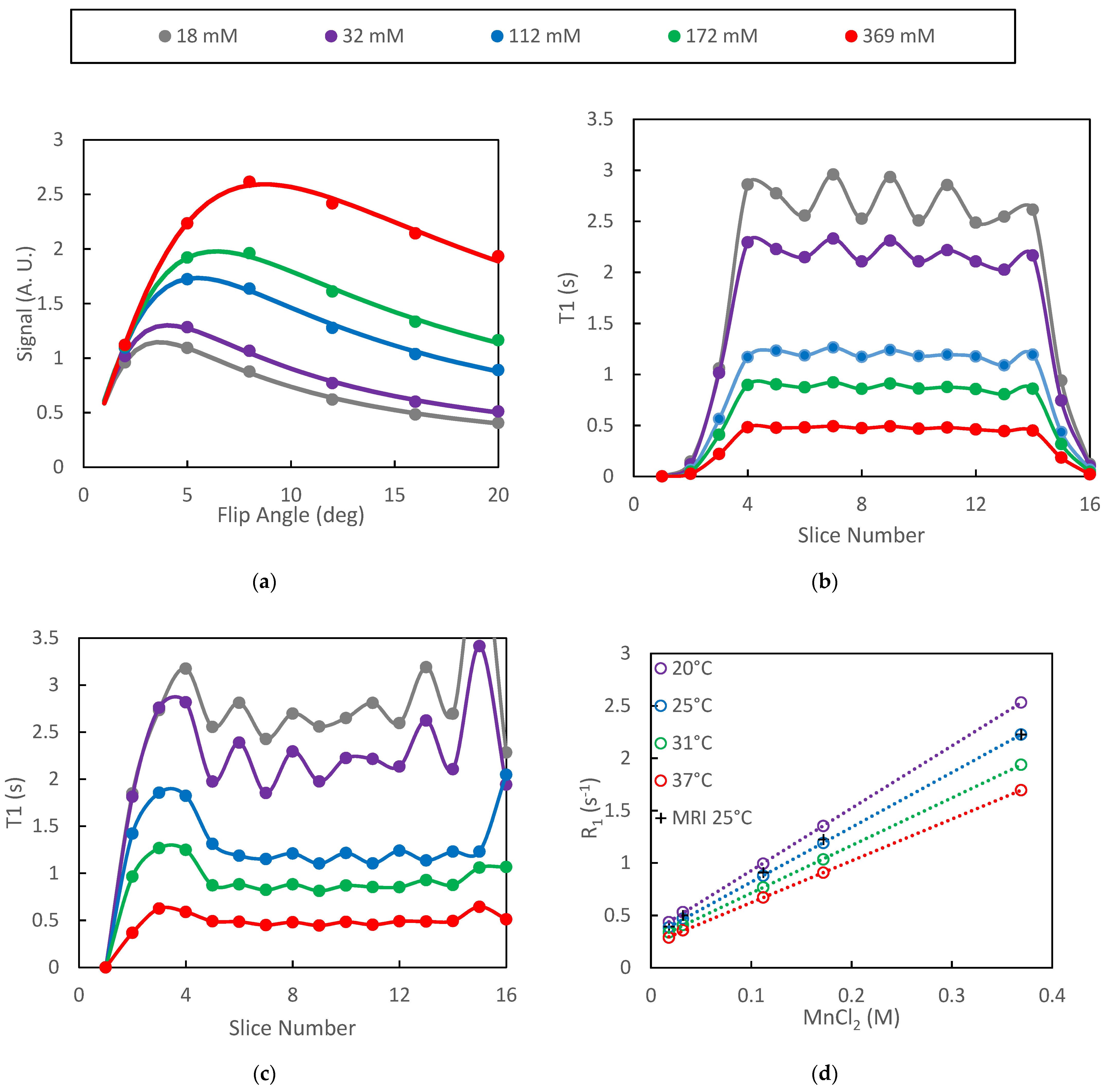
3.1. Phantom Studies
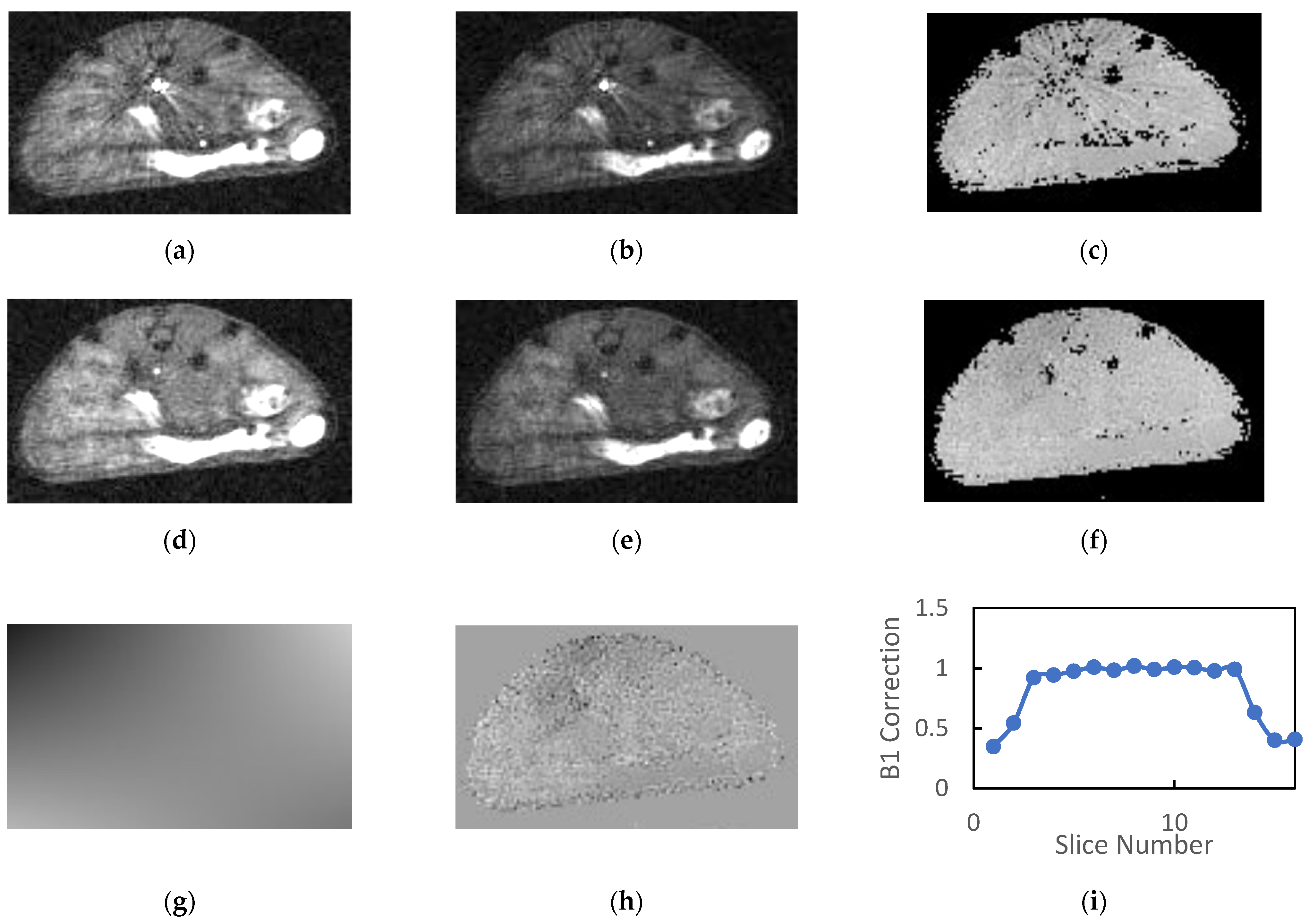
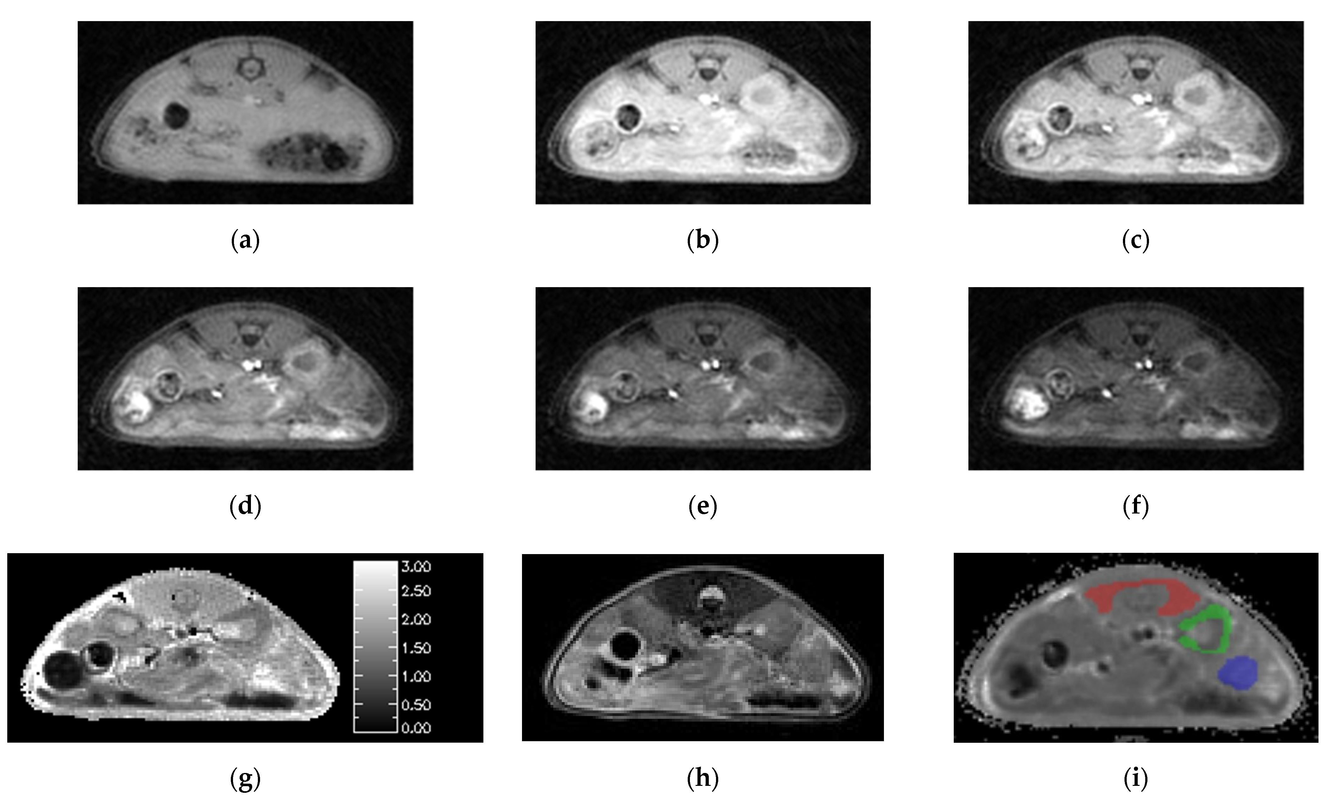
AFI studies of the phantom array were used to determine the spoiler gradient parameters necessary to assure suppression of transverse magnetization between repetitions and assess the accuracy of the T1 mapping protocol. The AFI implementation employed in the current study uses a loop structure in which the acquisition portion of the sequence is repeated six times with the RF pulse enabled on only the first two passes [37] resulting in an effective TR ratio of 5:1. In our implementation, the receiver is enabled for every pass through the loop. The data from the first two passes was used for calculation of the field maps and the remaining data provides a measure of spoiling efficiency. Any signal observed in the third or later passes is due to incomplete spoiling. The spoiler gradient area increased gradually until the signal acquired in the third pass was below noise levels for the phantom array. Complete suppression of signal was achieved with a spoiler applied on the slice axis of duration 3 ms and amplitude 16 g/cm (gradient area: Ag = 480 mT ms/m). This requirement for a large spoiling gradient is consistent with previously published simulated and experimental optimizations of the spoiler gradient for the AFI method [38]. There it was demonstrated that accurate B1 estimates are achieved independent of RF spoiling phase angle increment with Ag = 459 mT ms/m and a TR = 20 ms for samples with T2 = 37 ms. The modestly larger Ag required here is likely due to the longer transverse relaxation times of the phantoms employed in the current study.
Both the SoS AFI and VFA protocols yielded images of the phantoms that were free of artifacts and had a SNR in the range of 12–46. The estimated B1 corrections for the phantom studies were very flat in the transverse dimensions with mean values that ranged from 0.95 to 1.01 indicating accurate B1 calibration. The variation of B1 correction with respect to slice number reflects the response profile of the RF pulse used for observation, with a broad plateau region that drops off sharply near the edges of the FOV (data not shown). The estimated B1 correction within the plateau region of the pulse oscillated ±3% with respect to slice number which is somewhat larger than expected based on simulations of the response profile or the RF pulse used for excitation.
Plots of mean signal intensity from the VFA protocol as a function of flip angle were well characterized by least-squares fits to Equation (3) for all of the phantoms (Figure 1a). In the figure, the points are the mean VOI signal intensities averaged over the plateau slices (slices 4–14) and the solid lines are the model fits. Inclusion of B1 correction did not significantly alter the quality of the fits in the plateau region of the slab as the true/nominal B1 ratio was approximately 1.0 for those slices. The absence of systematic differences between the model and the measured data is an indication of spoiling efficacy in the VFA protocol [39]. The range of T1 values represented by the phantoms spans that which is expected for in-vivo DCE studies while the range of T2 values (28–300 ms) is larger than those expected in-vivo. The optimized spoiling gradient parameters are therefore expected to be adequate for our in-vivo studies.
The signal intensity generated by the VFA protocol was found to oscillate with respect to slice number in the plateau region of the selected slab. This oscillation propagated to the relaxation time estimates and increased in amplitude as T1 increased (Figure 1b). Inclusion of the B1 correction did not significantly alter the T1 estimates in the plateau slices but did extend the number of slices for which T1 estimates were be generated (Figure 1c).
The spectroscopically determined T1 estimates generated on different days were highly repeatable with standard deviations of approximately 1% (n = 3) of the measured T1 values. Plots of the spectroscopically determined relaxation rates vs. concentration were very linear (R2 = 0.999) for all temperatures studied (Figure 1d). Linear regression of the spectroscopic data yielded relaxivities of MnCl2 of 5.96, 5.23, 4.55 and 3.99 s−1 mm−1 for temperatures of 20, 25, 31 and 37 °C, respectively. These results are slightly higher than previously reported values of 5.0 and 3.9 s−1 mm−1 at 20 and 37 °C, respectively [40]. The relaxation rates as determined by the SoS-VFA protocol fall directly over those determined spectroscopically at 25 °C (Figure 1d) therefore demonstrating the accuracy afforded by the VFA technique.

3.2. Animal Studies

A total of 22 animals were examined, of which 19 were scanned with AFI both with and without OVS. The animals tolerated the 30–40 min protocol well with no adverse events and recovered from anesthesia quickly. Typical AFI images generated without OVS and their corresponding B1 maps are shown in Figure 2a–c. The TR1 and TR2 images in the figure have approximately equal windowing and are free of respiratory motion artifacts. The mean SNR (n = 19) for muscle/kidney/tumor was 7.6/9.3/7.9 and 7.4/8.7/7.3 for the TR1 and TR2 images, respectively. If windowed such that the background level is visible, there is clearly artifactual signal in the background regions of the images which contributes the noise estimates and reduces the reported SNR values. As such these values represent a lower limit for the SNR.
As noted previously, the reconstructed AFI images exhibited a large dynamic range due to the combination of large flip angle, short TR and inflowing unsaturated blood in the great vessels. The blood in the great vessels typically had an intensity that is 5–10 times greater than that of the static tissue. When these images were windowed appropriately for observation of the tissues, streaking artifacts radiating from the great vessels were observed in the reconstructed images as is evident in Figure 2a–c.
The calculated field maps were very flat within each slice indicating the high degree of transverse homogeneity of the RF volume coil. However, the streaking artifacts present in the source images were somewhat amplified in the calculated B1 maps (Figure 2c). The mean B1 correction values in plateau region of the slab (slices 4–13) was consistently close to but greater than unity (1.07 ± 0.04, n = 19).
Inclusion of OVS in the AFI protocol significantly reduced the signal intensity of blood in the great vessels and eliminated the streaking artifacts in both the source images and the calculated B1 maps (Figure 2d–f). The mean SNR (n = 19) for muscle/kidney/tumor was 11.0/13.2/11.5 and 10.9/12.1/10.3 for the TR1 and TR2 images, respectively. This represents a 37 to 45% gain in SNR relative to images acquired without OVS.
The 2D polynomial fits of the field maps provided a very accurate model of the calculated B1 field (Figure 2g). Note the figure is windowed to accentuate spatial variation. The magnitude of the spatial variation is actually quite small relative to the homogeneous component indicating a high degree of homogeneity in the transverse dimensions. This is also indicated by the fact that the mean values for the high order parameters in the polynomial fit were consistently two or more orders of magnitude smaller than the zero-order parameter (b0). Mean residues between the B1 correction maps and their polynomial fits were approximately 1% of the B1 correction and had minimal spatial variation for all slices within the plateau region of the slab (Figure 2h).
Plots of mean normalized B1 vs. slice number (Figure 2i) were flat for the center 8–10 slices and dropped off precipitously at the edges of the imaging slab. These plots reflect the product of the slice profile and the axial variation in RF coil sensitivity. Note the slab thickness was set to 85% of the FOV in the slice direction in order to minimize wrap around effects in the slice dimension. The inclusion of OVS and longer TR employed in the OVS studies had a minimal impact on the mean B1 estimates in the plateau region of the slab. The mean B1 correction with outer volume saturation (n = 19) was 1.10 ± 0.05 and ranged from 0.95 to 1.14.
Animal studies using the SoS-VFA T1 mapping protocol yielded images free of respiratory motion artifacts (Figure 3a–f). The images in the figure use identical windowing in order to highlight the flip-angle dependence of the signal intensity. There was no need to employ OVS in the VFA protocol due to the use of significantly lower flip angles than those employed in the AFI protocol. The mean SNR for the VFA images acquired with flip = 8° for the three tissues of interest was muscle/kidney/tumor = 23.3/30.2/25.5. We use 8° flip data for SNR estimation in the VFA protocol because it facilitates comparison to the dynamic data which are acquired with a comparable flip angle. The least-squares fits to Equation (3) were free from systematic errors and yielded high quality T1 maps (Figure 3g).
The T2 weighted images provided good resolution and high contrast between tumor and healthy tissues (Figure 3h). However, slight mis-registration between the T2 weighted and SoS images in the slice dimension were occasionally observed which motivated use of the DCE images for ROI definition. Boundaries for the ROIs were readily identified by simultaneously viewing the T1 maps and T2 weighted images. The resulting ROIs for muscle, kidney cortex and tumor are overlayed on one of the dynamic images from the corresponding study (Figure 3i).
For each VFA data set acquired both with and without OVS, T1 maps were generated three different ways in order to assess the impact of the various parameter estimation methods. T1 maps were calculated: (1) without B1 correction, (2) with B1 correction, and (3) with B1 correction that employed OVS. A comparison between the three approaches to estimating T1 is shown in the whisker plots of Figure 4 for each of the VOIs of interest. Mean T1 and standard deviations are also summarized in Table 1. The addition of B1 correction resulted in a statistically significant increase in the estimated T1 value for all three tissue types (t-test p less than 0.0001) while the addition of OVS did not significantly alter the T1 estimates (t-test p = 0.849/0.503/0.256 muscle/kidney/tumor) or their standard deviation. The addition of B1 correction to the T1 analysis is believed to provide more accurate T1 values since the B1 correction factor of ~1.07 was highly reproducible. The T1 estimates generated using the B1 correction with OVS enabled were therefore used to analyze the dynamic data.
Representative images from the SoS-DCE protocol prior to bolus arrival (a), at the bolus peak (b) and during washout (c) are shown in Figure 5. Identical windowing was employed each image in the figure. The images are of high SNR and free from motion artifacts. Prior to bolus arrival, mean (n = 22) image SNR for the tissues of interest was muscle/kidney/tumor = 9.4/11.6/9.9. Minimal degradation in image quality relative to the AFI and VFA data was evident due to the use of the KWIC sampling/view-sharing scheme [31]. Though not evident in the figure, streaking artifacts were occasionally observed in the images corresponding the maximum in the bolus due to the large dynamic range between the signal in the great vessels and the surrounding tissue.
Plots of VOI mean signal intensity vs. time for the three tissues of interest from the dynamic series had high SNR and the expected time dependence. The signal from the highly perfused kidney cortex (green, Figure 5d) consistently rose from baseline to its maximum in approximately 10 s (2–3 frames) and had a sharp peak. The peak in the kidney signal was followed by a rapid signal decline resembling an exponential decay to approximately 60% of the peak intensity with a time constant of ~20 s. The remaining signal washed out with a rate on the order of several minutes. The tissue response curve for muscle (red, Figure 5d) exhibited a much slower wash-in phase than kidney with typical time to maximum on the order of 60 s and the observed change in signal intensity was on the order of 20% of that observed for kidney. The form of the muscle and kidney tissue response curves were highly reproducible between voxels within the VOI and between animals.
The tissue response curves for tumor (blue, Figure 5d) were more variable both within a given tumor and between animals than those observed for normal tissues. The time to maximum for the tumor signal fell between those observed for kidney and muscle. Maps of Ktrans and ve were heterogeneous within the tumor (Figure 5e,f) with elevated levels around the periphery relative to the tumor core. Mean values (n = 22) of Ktrans and ve were 0.74 ± 0.19 min−1 (mean ± standard deviation) and 0.38 ± 0.14 for kidney and 0.21 ± 0.12 min−1 and 0.31 ± 0.17 for tumor relative to reference muscle Ktrans and ve set at 0.1 min−1 and 0.1, respectively.

4. Discussion

We have demonstrated a DCE-MRI protocol suitable for observation of deep-lying tumors in the abdomen of mice. The protocol consists of three scans, specifically: (1) B1 mapping with actual flip-angle imaging, (2) variable flip angle T1 mapping and (3) the dynamic series. All three scans employ a stack-of-stars sampled spoiled gradient echo acquisition. This sampling scheme has multiple advantages in the context of DCE imaging. The over sampling of the center of k-space afforded by SoS sampling makes the scan robust with regard to corruption by respiratory motion. In addition, the sampling scheme is amenable to view-sharing reconstruction techniques such as KWIC [31] which allow tradeoffs between spatial and temporal resolution to be made during image reconstruction of the dynamic data. Our method is a direct translation of the previously demonstrated clinical technique for DCE in the chest to abdominal studies in mice [27] without the use of self-gated respiratory phase binning for motion compensation. The motion correction methods used in the clinical study are not feasible in small animals because the interval between consecutive samples of the center of k-space is long relative to the respiration period in small animals. The present study relies on the oversampling of the center of k-space and fact that the magnitude of the respiration motion is significantly reduced in the abdomen of anesthetized animals relative to that in the chest.
Small-animal cardiac studies employing SoS sampling combined with navigator echoes have also been demonstrated. This method relies on performing multiple repetitions and using the navigator data to partition the acquired data into different cardiac phases. This approach motion compensation does not translate to the current study due to the single pass nature of the DCE protocol.
One limitation of the radial sampling scheme is that reconstruction of data sets with a large dynamic range often results in streaking artifacts. The combination of large flip angle and inflow of unsaturated blood in the great vessels resulted in such artifacts in the AFI protocol. We have demonstrated that these artifacts are readily eliminated by application of OVS techniques.
The impact of B1 correction, both with and without OVS, on the T1 estimates was also investigated. The corrections were minimal in phantom studies and had an insignificant impact on the T1 estimates. However, in the animal studies the AFI measurements revealed a consistent underestimation of the RF power by approximately 7% in the plateau region of the excitation pulse. The magnitude of this underestimation was not significantly affected by the addition of OVS. However, the addition of OVS did improve the SNR and overall image quality in the AFI scans. A failure to account for the underestimation of RF power was shown to result in an underestimation of T1 in the VFA study. For the equipment used in the current study, the under estimation of RF power appears to be due to inaccuracy in the RF power calibration routine. As such it is possible that use of an alternate power calibration method may eliminate the need for the B1 mapping protocol therefore reducing the total acquisition time of the DCE exam.
The combination of SoS sampling and KWIC image reconstruction yielded high-resolution images (matrix = 128 × 128 × 16) with a temporal resolution of 4.3 s with minimal reduction in image quality relative to fully sampled data. The resulting tissue response curves were well characterized by the reference tissue model. Maps of Ktrans and ve were relatively homogeneous within kidney cortex while a pattern of elevated Ktrans in tumor periphery relative to the core was observed in many KPC tumors.
Several DCE studies of the abdominal organs in mice have been previously reported including examination of pancreas [41,42,43,44], placenta [45,46], kidney [24,47] and liver [2,48,49,50,51]. Most of these studies employed full Cartesian sampling for acquisition of the dynamic data. The combined temporal and spatial resolution that can be achieved in the dynamic series with this approach is significantly lower than that presented in the current study. Improvements in resolution for Cartesian sampled DCE data may be achieved by application of keyhole acquisition methods [24] or compresses sensing image reconstruction [52,53]. However, the resulting dynamic data are often corrupted by motion artifacts. A variety of approaches for minimization of motion artifacts have also been proposed including securing the tissue of interest with a plastic platen [41], prospective gating [18], non-affine image registration [42] and use of navigator echoes [49]. Though application of these methods generally reduces the frequency of occurance of motion artifacts, some data corruptoin persists.
A limited number of authors have taken advantage of the motion robustness of radial samping for acqusition of abdominal DCE data in mouse models. Both radial 3D gradient echo (3D-GRE) [48] and ultra-short echo time (UTE) [47] methods have been used to generate dynaimc data. These techniques provide robustness to motioin artifacts that is comparable to the metods presented in the current report. In addition, these methods provide higher temporal and spatial resoltuion than can be achieved with Cartesian sampling when combined with view-sharing image reconstruction methods. The UTE method has the added advantage of minimizing T2 * contributions to the observed signal changes. However, the SoS sampling scheme employed in the current study requires fewer views per image than the radial 3D GRE and the UTE methods. SoS sampling also provides greater flexibility with regard to extent and resolution in the slice dimension. This flexibility can be used to minimize the extent of the acquired data to include only the tissue of interest. These factors in turn result in higher temporal and/or spatial resolution provided by the SoS scheme than can be achieved with the 3D radial methods for a given TR.
The results presented in here highlight both the advantages and the limitations of the radial sampling techniques in the context of dynamic imaging. As is evident in the images presented, motion artifacts in radially sampled data do not manifest as coherent ghosts as is the case Cartesian sampling. Less evident in the data presented is the fact that image corruption due to motion as well as B0 inhomogeneity is present in the images in the form of incoherent artifacts spread throughout the images. Here it was noted that such artifacts interfered with our SNR estimates. Simultaneously, the lack of systematic errors between the observed data and the models employed suggests that such artifacts do not significantly interfere with the tissue signals. Further improvements in image quality may be achieved using self-gating techniques to eliminate views that are corrupted by motion and through the use of artificial intelligence image reconstruction techniques to correct for the effects of B0 inhomogeneity.

5. Conclusions

We have demonstrated a DCE-MRI method that uses golden-angle SoS sampling throughout with KWIC image reconstruction for the dynamic data. This is the first time this method of acquisition of DCE data has been demonstrated in small-animal models. The resulting protocol provides high spatial (matrix = 128 × 128 × 16) and temporal (4.3 s) resolution and minimal sensitivity to motion artifacts. The technique was demonstrated in an orthotopic mouse model of pancreatic ductal adenocarcinoma, and the resulting data were analyzed using the reference tissue method. The resulting method was shown to provide high-resolution maps of Ktrans and ve in this model.

Author Contributions

Conceptualization: R.Z., S.P.; Methodology: S.P., H.K.S. and M.R.; Software: S.P., H.K.S. and M.R.; Validation: S.P., H.K.S. and M.R.; Data analysis: S.P., M.R., M.G. and H.K.S.; Resources: R.Z.; Writing-original draft preparation: S.P.; Writing-review and editing: all authors; Visualization: S.P., M.R. and R.Z.; Supervision and Program administration: S.P. and R.Z.; Funding acquisition: R.Z. All authors have read and agreed to the published version of the manuscript.

Funding

This study was partly supported by the Penn Quantitative Imaging Resource for Pancreatic Cancer (NIH: U24-CA-231858). The Small-Animal Imaging Facility at the University of Pennsylvania is supported by the Abramson Cancer Center (NIH: P30-CA-916529).

Institutional Review Board Statement

The animal studies were reviewed and approved by the Institutional Animal Care and Use Committee of University of Pennsylvania.

Informed Consent Statement

Not applicable.

Data Availability Statement

Data supporting the results of this study will be deposited at the GitHub open-source platform (https://pennpancreaticcancerimagingresource.github.io/data.html (accessed on 6 May 2022)) upon the publication of the paper.

Acknowledgments

We thank Cynthia Clendenin, DVM for providing the KPC mice bred at the Mouse Hospital of the Abramson Cancer Center University of Pennsylvania and Hoon Choi for technical assistance.

Conflicts of Interest

The authors declare no conflict of interest.

References

  1. Montelius, M.; Spetz, J.; Jalnefjord, O.; Berger, E.; Nilsson, O.; Ljungberg, E. Forssell-Aronsson, Identification of Potential MR Derived Biomarkers for Tumor Tissue Response to Lu-177-Octreotate Therapy in an Animal Model of Small Intestine Neuroendocrine Tumor. Transl. Oncol. 2018, 11, 193–204. [Google Scholar] [CrossRef]
  2. Yamada, T.; Kashiwagi, Y.; Rokugawa, T.; Kato, H.; Konishi, H.; Hamada, T.; Nagai, R.; Masago, Y.; Itoh, M.; Suganami, T.; et al. Evaluation of hepatic function using dynamic contrast-enhanced magnetic resonance imaging in melanocortin 4 receptor-deficient mice as a model of nonalcoholic steatohepatitis. Magn. Reson. Imaging 2019, 57, 210–217. [Google Scholar] [CrossRef] [PubMed]
  3. Montelius, M.; Jalnefjord, O.; Spetz, J.; Nilsson, O.; Forssell-Aronsson, E.; Ljungberg, M. Multiparametric MR for non-invasive evaluation of tumour tissue histological characteristics after radionuclide therapy. Nmr Biomed. 2019, 32, 14. [Google Scholar] [CrossRef]
  4. O’Connor, J.P.B.; Jackson, A.; Parker, G.J.M.; Roberts, C.; Jayson, G.C. Dynamic contrast-enhanced MRI in clinical trials of antivascular therapies. Nat. Rev. Clin. Oncol. 2012, 9, 167–177. [Google Scholar] [CrossRef] [PubMed]
  5. Consolino, L.; Longo, D.L.; Sciortino, M.; Dastru, W.; Cabodi, S.; Giovenzana, G.B.; Aime, S. Assessing tumor vascularization as a potential biomarker of imatinib resistance in gastrointestinal stromal tumors by dynamic contrast-enhanced magnetic resonance imaging. Gastric Cancer 2017, 20, 629–639. [Google Scholar] [CrossRef] [PubMed]
  6. Bi, S.X.; Li, X.H.; Wei, C.S.; Xiang, H.H.; Shen, Y.X.; Yu, Y.Q. The antitumour growth and antiangiogenesis effects of xanthatin in murine glioma dynamically evaluated by dynamic contrast-enhanced magnetic resonance imaging. Phytother. Res. 2019, 33, 149–158. [Google Scholar] [CrossRef]
  7. Checkley, D.; Tessier, J.J.L.; Wedge, S.R.; Dukes, M.; Kendrew, J.; Curry, B.; Middleton, B.; Waterton, J.C. Dynamic contrast-enhanced MRI of vascular changes induced by the VEGF-signalling inhibitor ZD4190 in human tumour xenografts. Magn. Reson. Imaging 2003, 21, 475–482. [Google Scholar] [CrossRef]
  8. Piludu, F.; Marzi, S.; Pace, A.; Villani, V.; Fabi, A.; Carapella, C.M.; Terrenato, I.; Antenucci, A.; Vidiri, A. Early biomarkers from dynamic contrast-enhanced magnetic resonance imaging to predict the response to antiangiogenic therapy in high-grade gliomas. Neuroradiology 2015, 57, 1269–1280. [Google Scholar] [CrossRef]
  9. Sweis, R.F.; Medved, M.; Towey, S.; Karczmar, G.S.; Oto, A.; Szmulewitz, R.Z.; O’Donnell, P.H.; Fishkin, P.; Karrison, T.; Stadler, W.M. Dynamic Contrast-Enhanced Magnetic Resonance Imaging as a Pharmacodynamic Biomarker for Pazopanib in Metastatic Renal Carcinoma. Clin. Genitourin. Cancer 2017, 15, 207–212. [Google Scholar] [CrossRef]
  10. Xue, W.; Du, X.S.; Wu, H.; Liu, H.; Xie, T.; Tong, H.P.; Chen, X.; Guo, Y.; Zhang, W.G. Aberrant glioblastoma neovascularization patterns and their correlation with DCE-MRI-derived parameters following temozolomide and bevacizumab treatment. Sci. Rep. 2017, 7, 10. [Google Scholar] [CrossRef]
  11. Fram, E.K.; Herfkens, R.J.; Johnson, G.A.; Glover, G.H.; Karis, J.P.; Shimakawa, A.; Perkins, T.G.; Pelc, N.J. Rapid Calculation of T1 Using Variable Flip Angle Gradient Refocused Imaging. Magn. Reson. Imaging 1987, 5, 201–208. [Google Scholar] [CrossRef]
  12. Cheng, H.L.M.; Wright, G.A. Rapid high-resolution T-1 mapping by variable flip angles: Accurate and precise measurements in the presence of radiofrequency field inhomogeneity. Magn. Reson. Med. 2006, 55, 566–574. [Google Scholar] [CrossRef] [PubMed]
  13. Bane, O.; Hectors, S.J.; Wagner, M.; Arlinghaus, L.L.; Aryal, M.P.; Cao, Y.; Chenevert, T.L.; Fennessy, F.; Huang, W.; Hylton, N.M.; et al. Accuracy, repeatability, and interplatform reproducibility of T-1 quantification methods used for DCE-MRI: Results from a multicenter phantom study. Magn. Reson. Med. 2018, 79, 2564–2575. [Google Scholar] [CrossRef] [PubMed]
  14. Yarnykh, V.L. Actual flip-angle imaging in the pulsed steady state: A method for rapid three-dimensional mapping of the transmitted radiofrequency field. Magn. Reson. Med. 2007, 57, 192–200. [Google Scholar] [CrossRef]
  15. Kim, J.; Moestue, S.A.; Bathen, T.F.; Kim, E. R2* Relaxation Affects Pharmacokinetic Analysis of Dynamic Contrast-Enhanced MRI in Cancer and Underestimates Treatment Response at 7 T. Tomography 2019, 5, 308–319. [Google Scholar] [CrossRef] [PubMed]
  16. Pitman, K.E.; Bakke, K.M.; Kristian, A.; Malinen, E. Ultra-early changes in vascular parameters from dynamic contrast enhanced MRI of breast cancer xenografts following systemic therapy with doxorubicin and liver X receptor agonist. Cancer Imaging 2019, 19, 88. [Google Scholar] [CrossRef] [PubMed]
  17. Liang, J.Y.; Cheng, Q.Q.; Huang, J.X.; Ma, M.J.; Zhang, D.; Lei, X.P.; Xiao, Z.Y.; Zhang, D.M.; Shi, C.Z.; Luo, L.P. Monitoring tumour microenvironment changes during anti-angiogenesis therapy using functional MRI. Angiogenesis 2019, 22, 457–470. [Google Scholar] [CrossRef]
  18. Cao, J.B.; Pickup, S.; Clendenin, C.; Blouw, B.; Choi, H.; Kang, D.; Rosen, M.; O’Dwyer, P.J.; Zhou, R. Dynamic Contrast-enhanced MRI Detects Responses to Stroma-directed Therapy in Mouse Models of Pancreatic Ductal Adenocarcinoma. Clin. Cancer Res. 2019, 25, 2314–2322. [Google Scholar] [CrossRef]
  19. Backhaus, P.; Buther, F.; Wachsmuth, L.; Frohwein, L.; Buchholz, R.; Karst, U.; Schafers, K.; Hermann, S.; Schafers, M.; Faber, C. Toward precise arterial input functions derived from DCE-MRI through a novel extracorporeal circulation approach in mice. Magn. Reson. Med. 2020, 84, 1404–1415. [Google Scholar] [CrossRef]
  20. Ge, X.; Quirk, J.D.; Engelbach, J.A.; Bretthorst, G.L.; Li, S.Q.; Shoghi, K.I.; Garbow, J.R.; Ackerman, J.J.H. Test-Retest Performance of a 1-Hour Multiparametric MR Image Acquisition Pipeline with Orthotopic Triple-Negative Breast Cancer Patient-Derived Tumor Xenografts. Tomography 2019, 5, 320–331. [Google Scholar] [CrossRef]
  21. Cardenas-Rodriguez, J.; Howison, C.M.; Pagel, M.D. A linear algorithm of the reference region model for DCE-MRI is robust and relaxes requirements for temporal resolution. Magn. Reson. Imaging 2013, 31, 497–507. [Google Scholar] [CrossRef] [PubMed]
  22. Yankeelov, T.E.; Luci, J.J.; Lepage, M.; Li, R.; Debusk, L.; Lin, P.C.; Price, R.R.; Gore, J.C. Quantitative pharmacokinetic analysis of DCE-MRI data without an arterial input function: A reference region model. Magn. Reson. Imaging 2005, 23, 519–529. [Google Scholar] [CrossRef] [PubMed]
  23. Kim, H.; Folks, K.D.; Guo, L.L.; Stockard, C.R.; Fineberg, N.S.; Grizzle, W.E.; George, J.F.; Buchsbaum, D.J.; Morgan, D.E.; Zinn, K.R. DCE-MRI Detects Early Vascular Response in Breast Tumor Xenografts Following Anti-DR5 Therapy. Mol. Imaging Biol. 2011, 13, 94–103. [Google Scholar] [CrossRef] [PubMed]
  24. Jiang, K.; Tang, H.; Mishra, P.K.; Macura, S.I.; Lerman, L.O. Measurement of murine kidney functional biomarkers using DCE-MRI: A multi-slice TRICKS technique and semi-automated image processing algorithm. Magn. Reson. Imaging 2019, 63, 226–234. [Google Scholar] [CrossRef] [PubMed]
  25. Subashi, E.; Moding, E.J.; Cofer, G.P.; MacFall, J.R.; Kirsch, D.G.; Qi, Y.; Johnson, G.A. A comparison of radial keyhole strategies for high spatial and temporal resolution 4D contrast-enhanced MRI in small animal tumor models. Med. Phys. 2013, 40, 10. [Google Scholar] [CrossRef]
  26. Gu, Y.N.; Gao, H.Y.; Kim, K.; Liu, Y.C.; Ramos-Estebanez, C.; Luo, Y.; Wang, Y.M.; Yu, X. Dynamic oxygen-17 MRI with adaptive temporal resolution using golden-means-based 3D radial sampling. Magn. Reson. Med. 2021, 85, 3112–3124. [Google Scholar] [CrossRef]
  27. Lin, W.; Guo, J.Y.; Rosen, M.A.; Song, H.K. Respiratory Motion-Compensated Radial Dynamic Contrast-Enhanced (DCE)-MRI of Chest and Abdominal Lesions. Magn. Reson. Med. 2008, 60, 1135–1146. [Google Scholar] [CrossRef]
  28. Trotier, A.J.; Castets, C.R.; Lefrancois, W.; Ribot, E.J.; Franconi, J.M.; Thiaudiere, E.; Miraux, S. USPIO-enhanced 3D-cine self-gated cardiac MRI based on a stack-of-stars golden angle short echo time sequence: Application on mice with acute myocardial infarction. J. Magn. Reson. Imaging 2016, 44, 355–365. [Google Scholar] [CrossRef]
  29. Hingorani, S.R.; Petricoin, E.F.; Maitra, A.; Rajapakse, V.; King, C.; Jacobetz, M.A.; Ross, S.; Conrads, T.P.; Veenstra, T.D.; Hitt, B.A.; et al. Preinvasive and invasive ductal pancreatic cancer and its early detection in the mouse. Cancer Cell 2003, 4, 437–450. [Google Scholar] [CrossRef]
  30. DPeters, C.; Korosec, F.R.; Grist, T.M.; Block, W.F.; Holden, J.E.; Vigen, K.K.; Mistretta, C.A. Undersampled projection reconstruction applied to MR angiography. Magn. Reson. Med. 2000, 43, 91–101. [Google Scholar] [CrossRef]
  31. Song, H.K.; Dougherty, L. k-space weighted image contrast (KWIC) for contrast manipulation in projection reconstruction MRI. Magn. Reson. Med. 2000, 44, 825–832. [Google Scholar] [CrossRef]
  32. Zur, Y.; Wood, M.L.; Neuringer, L.J. Spoiling of Transverse Magnetization in Steady-State Sequences. Magn. Reson. Med. 1991, 21, 251–263. [Google Scholar] [CrossRef] [PubMed]
  33. Winkelmann, S.; Schaeffter, T.; Koehler, T.; Eggers, H.; Doessel, O. An optimal radial profile order based on the golden ratio for time-resolved MRI. IEEE Trans. Med. Imaging 2007, 26, 68–76. [Google Scholar] [CrossRef] [PubMed]
  34. Schneider, C.A.; Rasband, W.S.; Eliceiri, K.W. NIH Image to ImageJ: 25 years of image analysis. Nat. Methods 2012, 9, 671–675. [Google Scholar] [CrossRef]
  35. Jones, K.M.; Pagel, M.D.; Cárdenas-Rodríguez, J. Linearization improves the repeatability of quantitative dynamic contrast enhanced MRI. Magn. Reson. Imaging 2018, 47, 16–24. [Google Scholar] [CrossRef]
  36. Makihara, K.; Yamaguchi, M.; Ito, K.; Sakaguchi, K.; Hori, Y.; Semba, T.; Funahashi, Y.; Fujii, H.; Terada, Y. New Cluster Analysis Method for Quantitative Dynamic Contrast-Enhanced MRI Assessing Tumor Heterogeneity Induced by a Tumor-Microenvironmental Ameliorator (E7130) Treatment to a Breast Cancer Mouse Model. J. Magn. Reson. Imaging 2022. (Online ahead of print). [Google Scholar] [CrossRef]
  37. Nehrke, K. On the Steady-State Properties of Actual Flip Angle Imaging (AFI). Magn. Reson. Med. 2009, 61, 84–92. [Google Scholar] [CrossRef]
  38. Yarnykh, V.L. Optimal Radiofrequency and Gradient Spoiling for Improved Accuracy of T(1) and B(1) Measurements Using Fast Steady-State Techniques. Magn. Reson. Med. 2010, 63, 1610–1626. [Google Scholar] [CrossRef]
  39. Helms, G.; Dathe, H.; Weiskopf, N.; Dechent, P. Identification of Signal Bias in the Variable Flip Angle Method by Linear Display of the Algebraic Ernst Equation. Magn. Reson. Med. 2011, 66, 669–677. [Google Scholar] [CrossRef]
  40. Watanabe, T.; Frahm, J.; Michaelis, T. Reduced intracellular mobility underlies manganese relaxivity in mouse brain in vivo: MRI at 2.35 and 9.4 T. Brain Struct. Funct. 2015, 220, 1529–1538. [Google Scholar] [CrossRef]
  41. Kim, H.; Folks, K.D.; Guo, L.L.; Sellers, J.C.; Fineberg, N.S.; Stockard, C.R.; Grizzle, W.E.; Buchsbaum, D.J.; Morgan, D.E.; George, J.F.; et al. Early Therapy Evaluation of Combined Cetuximab and Irinotecan in Orthotopic Pancreatic Tumor Xenografts by Dynamic Contrast-Enhanced Magnetic Resonance Imaging. Mol. Imaging 2011, 10, 153–167. [Google Scholar] [CrossRef] [PubMed]
  42. Wu, L.; Lv, P.; Zhang, H.T.; Fu, C.X.; Yao, X.Z.; Wang, C.; Zeng, M.S.; Li, Y.Y.; Wang, X.L. Dynamic contrast-enhanced (DCE) MRI assessment of microvascular characteristics in the murine orthotopic pancreatic cancer model. Magn. Reson. Imaging 2015, 33, 737–760. [Google Scholar] [CrossRef] [PubMed]
  43. Wu, L.; Wang, C.; Yao, X.Z.; Liu, K.; Xu, Y.J.; Zhang, H.T.; Fu, C.X.; Wang, X.L.; Li, Y.Y. Application of 3.0 Tesla Magnetic Resonance Imaging for Diagnosis in the Orthotopic Nude Mouse Model of Pancreatic Cancer. Exp. Anim. 2014, 63, 403–413. [Google Scholar] [CrossRef]
  44. Ritelli, R.; Ngaleu, R.N.; Bontempi, P.; Dandrea, M.; Nicolato, E.; Boschi, F.; Fiorini, S.; Calderan, L.; Scarpa, A.; Marzola, P. Pancreatic cancer growth using magnetic resonance and bioluminescence imaging. Magn. Reson. Imaging 2015, 33, 592–599. [Google Scholar] [CrossRef]
  45. Remus, C.C.; Sedlacik, J.; Wedegaertner, U.; Arck, P.; Hecher, K.; Adam, G.; Forkert, N.D. Application of the steepest slope model reveals different perfusion territories within the mouse placenta. Placenta 2013, 34, 899–906. [Google Scholar] [CrossRef] [PubMed]
  46. Alison, M.; Quibel, T.; Balvay, D.; Autret, G.; Bourillon, C.; Chalouhi, G.E.; Deloison, B.; Salomon, L.J.; Cuenod, C.A.; Clement, O.; et al. Measurement of Placental Perfusion by Dynamic Contrast-Enhanced MRI at 4.7 T. Investig. Radiol. 2013, 48, 535–542. [Google Scholar] [CrossRef] [PubMed]
  47. Privratsky, J.R.; Wang, N.; Qi, Y.; Ren, J.F.; Morris, B.T.; Hunting, J.C.; Johnson, G.A.; Crowley, S.D. Dynamic contrast-enhanced MRI promotes early detection of toxin-induced acute kidney injury. Am. J. Physiol.-Ren. Physiol. 2019, 316, F351–F359. [Google Scholar] [CrossRef]
  48. Vautier, J.; el Tayara, N.E.; Walczak, C.; Mispelter, J.; Volk, A. Radial multigradient-echo DCE-MRI for 3D K-trans mapping with individual arterial input function measurement in mouse tumor models. Magn. Reson. Med. 2013, 70, 823–828. [Google Scholar] [CrossRef]
  49. Byk, K.; Jasinski, K.; Bartel, Z.; Jasztal, A.; Sitek, B.; Tomanek, B.; Chlopicki, S.; Skorka, T. MRI-based assessment of liver perfusion and hepatocyte injury in the murine model of acute hepatitis. Magn. Reson. Mater. Phys. Biol. Med. 2016, 29, 789–798. [Google Scholar] [CrossRef]
  50. Sakata, N.; Obenaus, A.; Chan, N.K.; Hayes, P.; Chrisler, J.; Hathout, E. Correlation between angiogenesis and islet graft function in diabetic mice: Magnetic resonance imaging assessment. J. Hepato-Biliary-Pancreat. Sci. 2010, 17, 692–700. [Google Scholar] [CrossRef]
  51. Song, K.D.; Choi, D.; Lee, J.H.; Im, G.H.; Yang, J.; Kim, J.H.; Lee, W.J. Evaluation of Tumor Microvascular Response to Brivanib by Dynamic Contrast-Enhanced 7-T MRI in an Orthotopic Xenograft Model of Hepatocellular Carcinoma. Am. J. Roentgenol. 2014, 202, W559–W566. [Google Scholar] [CrossRef] [PubMed]
  52. Smith, D.S.; Welch, E.B.; Li, X.; Arlinghaus, L.R.; Loveless, M.E.; Koyama, T.; Gore, J.C.; Yankeelov, T.E. Quantitative effects of using compressed sensing in dynamic contrast enhanced MRI. Phys. Med. Biol. 2011, 56, 4933–4946. [Google Scholar] [CrossRef] [PubMed]
  53. Han, S.; Cho, H. Temporal Resolution Improvement of Calibration-Free Dynamic Contrast-Enhanced MRI With Compressed Sensing Optimized Turbo Spin Echo: The Effects of Replacing Turbo Factor with Compressed Sensing Accelerations. J. Magn. Reson. Imaging 2016, 44, 138–147. [Google Scholar] [CrossRef] [PubMed]
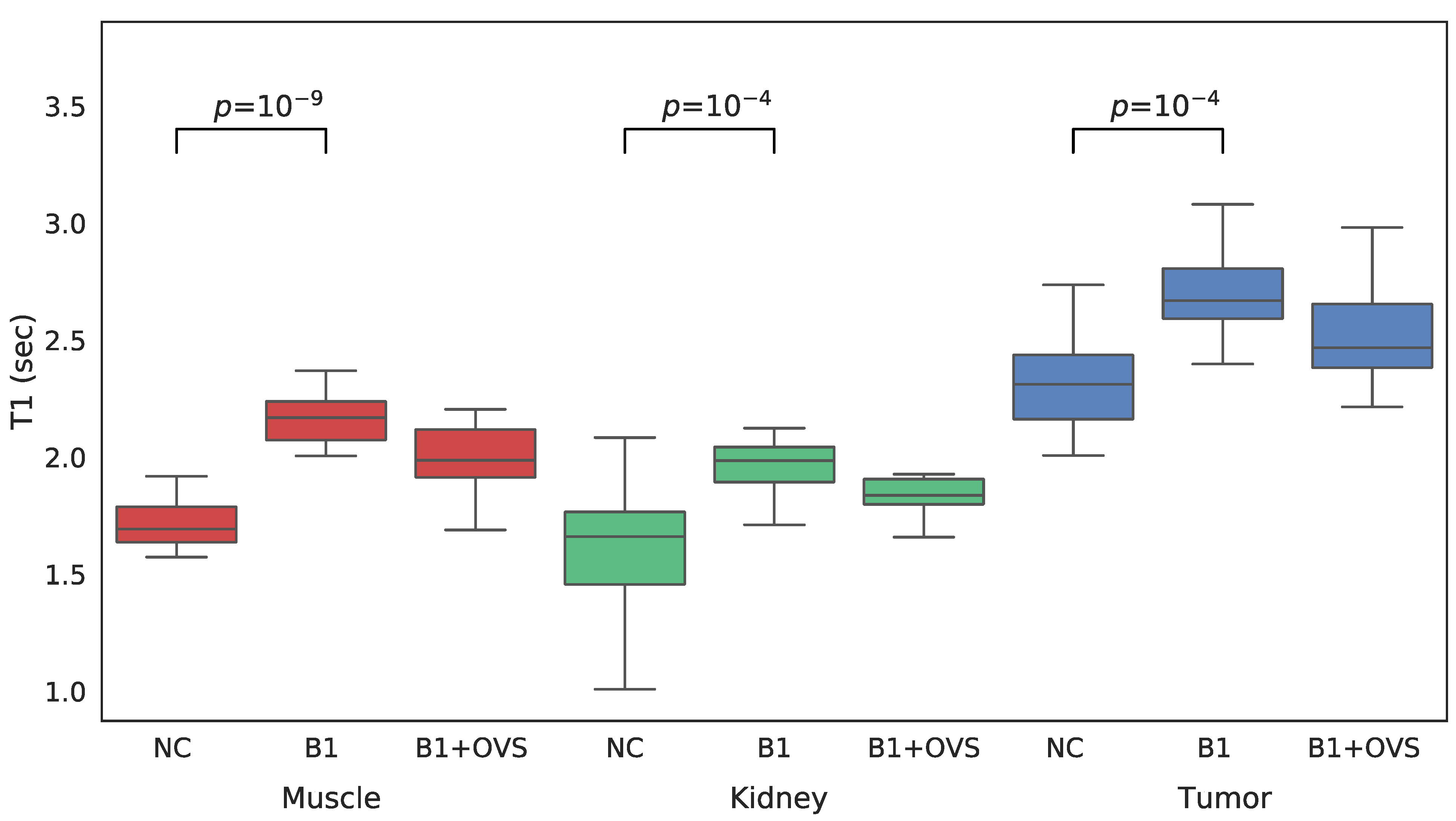
Figure 1. Data from VFA study of MnCl2 phantoms are presented: (a) ROI signal intensity vs. flip angles is accurately fit by the model; (b) oscillations in the mean T1 with respect to slice number increased with increasing T1; (c) inclusion of B1 correction increased the width of the T1 profile as well as amplified oscillations near the edge of the slab; (d) relaxation rate plots were highly linear both for the spectroscopic (inversion recovery) and VFA protocols.
Tomography 08 00178 g001
Figure 2. Typical images generated by the SoS AFI protocol are presented: (a) TR1 and (b) TR2 images generated without OVS exhibit streaking artifacts that propagate to the (c) B1 maps. The addition of OVS reduces the intensity of the blood signal in the great vessels for the (d) TR1 and (e) TR2 images therefore eliminating the previously observed streaking artifacts in the (f) B1 maps. The (g) fits of the B1 maps to a low order 2D polynomial exhibited no systematic errors and had (h) low homogeneous residues. (i) Plots of the normalized B1 estimates versus slice number reflect the product of the RF excitation profile and the longitudinal sensitivity of the coil.
Tomography 08 00178 g002
Figure 3. Images generated by the SoS-VFA protocol for flip angles of (a) 2, (b) 5, (c) 8, (d) 12, (e) 16 and (f) 20° were free of motion, had high SNR and yielded high quality (g) T1 maps. The (h) T2 weighted images provided good soft tissue contrast. VOI analysis was performed for three tissue types: (i) muscle (red), kidney (green) and tumor (blue).
Tomography 08 00178 g003
Figure 4. Whisker plots of SoS-VFA T1 estimates generated without B1 correction (NC), with B1 correction but no OVS (B1) and with B1 correction and OVS enabled (B1 + OVS) for muscle (left, red), kidney (center, green) and tumor (right, blue).
Tomography 08 00178 g004
Figure 5. Typical images from the SoS-DCE protocol (a) before bolus arrival, (b) at the bolus peak and (c) during washout are shown. (d) VOI response curves for muscle (red), kidney (green) and tumor (blue) had high SNR and the expected form. Maps of (e) Ktrans and (f) ve were elevated at the tumor periphery relative to the core. Color bar scales are min−1 for Ktrans and are unitless for ve.
Tomography 08 00178 g005
Table 1. Mean and standard deviations of T1 estimates (s) for the volumes of interest as generated using three different methods.
MethodMuscleKidneyTumor
No B1 Correction1.70 ± 0.111.60 ± 0.142.27 ± 0.19
B1 Correction w/o OVS2.14 ± 0.081.93 ± 0.122.69 ± 0.21
B1 Correction with OVS2.16 ± 0.071.87 ± 0.102.56 ± 0.19
Publisher’s Note: MDPI stays neutral with regard to jurisdictional claims in published maps and institutional affiliations.

