
Biologicalization of Smart Manufacturing Using DNA-Based Computing

Abstract
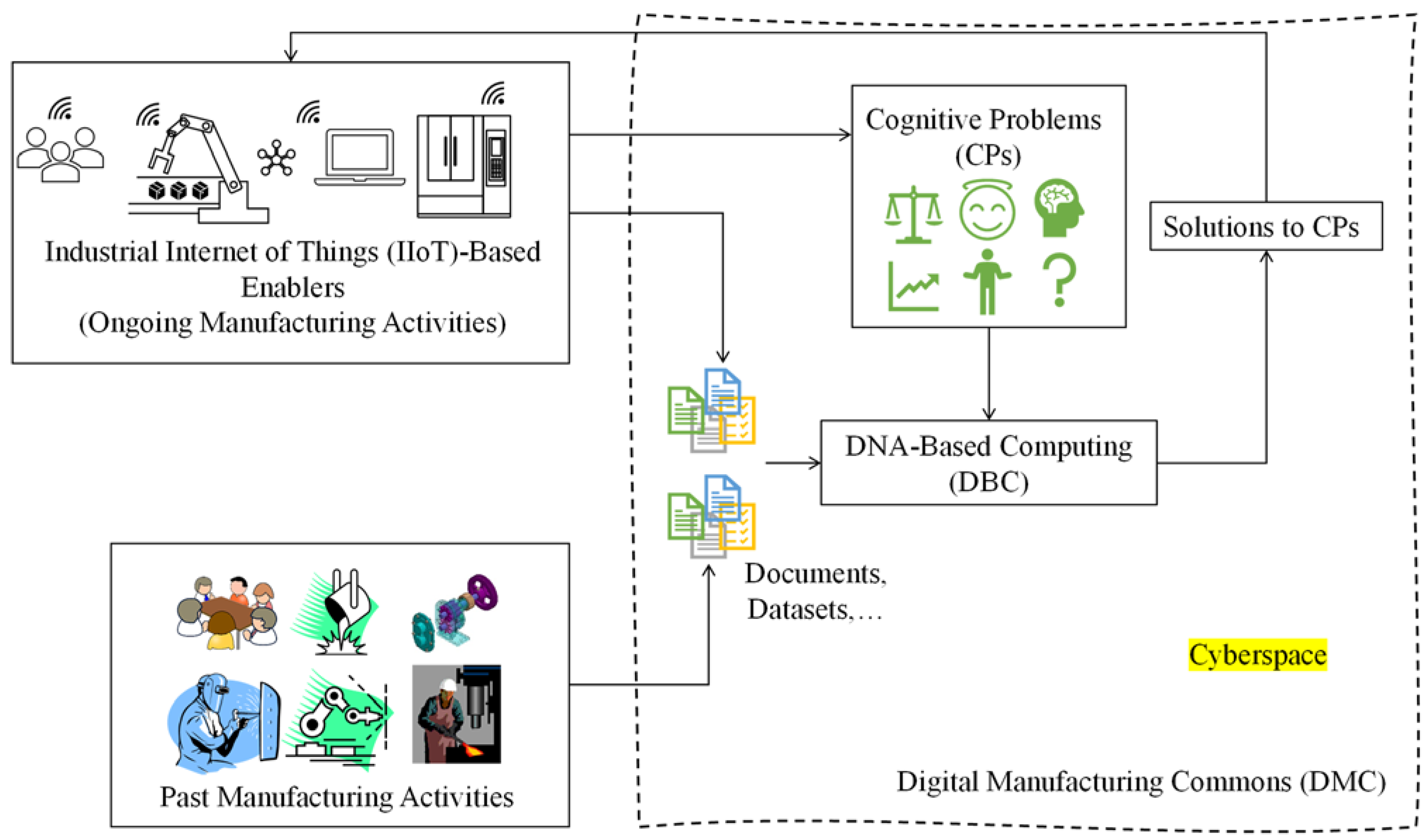
:1. Introduction
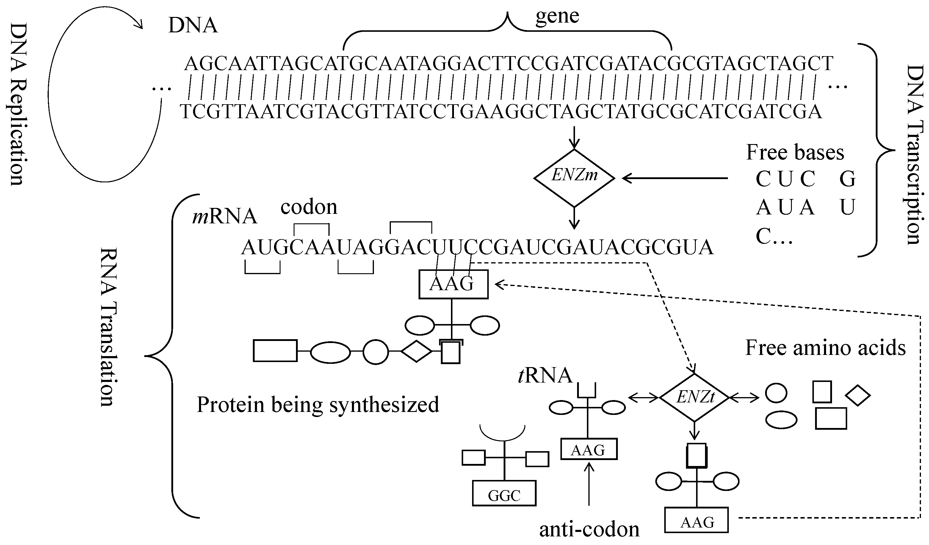
2. Central Dogma of Molecular Biology
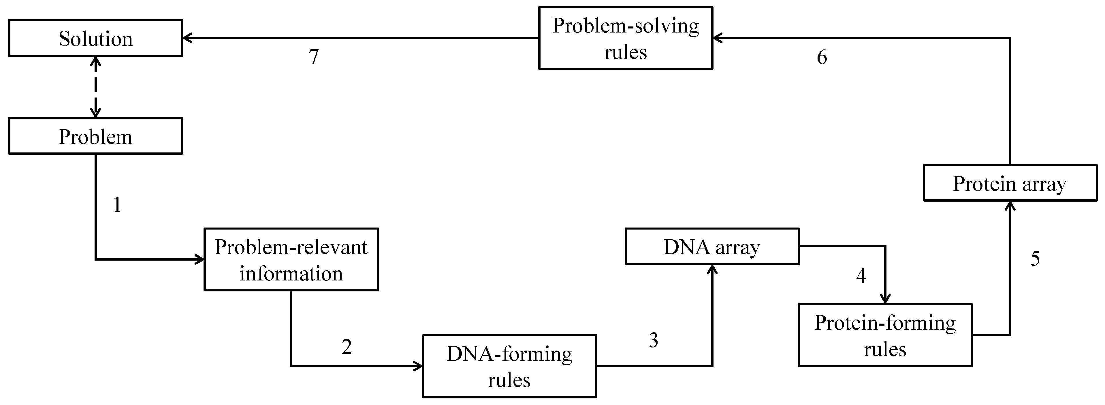
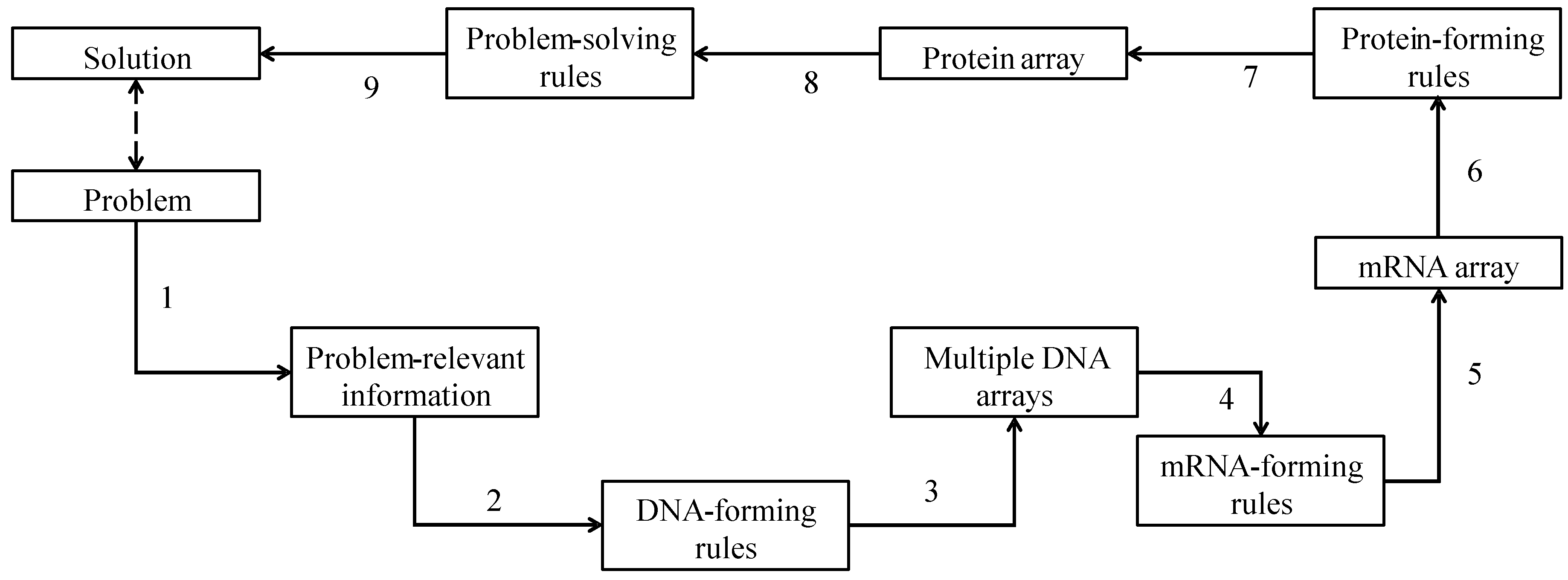
3. DNA-Based Computing (DBC)
- IF codon(k) ∈ {ATT, ATC, ATA} THEN protein(k) = I
- IF codon(k) ∈ {CTT, CTC, CTA, CTG, TTA, TTG} THEN protein(k) = L
- IF codon(k) ∈ {GTT, GTC, GTA, GTG} THEN protein(k) = V
- IF codon(k) ∈ {TTT, TTC} THEN protein(k) = F
- IF codon(k) ∈ {ATG} THEN protein(k) = M
- IF codon(k) ∈ {TGT, TGC} THEN protein(k) = C
- IF codon(k) ∈ {GCT, GCC, GCA, GCG} THEN protein(k) = A
- IF codon(k) ∈ {GGT, GGC, GGA, GGG} THEN protein(k) = G
- IF codon(k) ∈ {CCT, CCC, CCA, CCG} THEN protein(k) = P
- IF codon(k) ∈ {ACT, ACC, ACA, ACG} THEN protein(k) = T
- IF codon(k) ∈ {TCT, TCC, TCA, TCG, AGT, AGC} THEN protein(k) = S
- IF codon(k) ∈ {TAT, TAC} THEN protein(k) = Y
- IF codon(k) ∈ {TGG} THEN protein(k) = W
- IF codon(k) ∈ {CAA, CAG} THEN protein(k) = Q
- IF codon(k) ∈ {AAT, AAC} THEN protein(k) = N
- IF codon(k) ∈ {CAT, CAC} THEN protein(k) = H
- IF codon(k) ∈ {GAA, GAG} THEN protein(k) = E
- IF codon(k) ∈ {GAT, GAC} THEN protein(k) = D
- IF codon(k) ∈ {AAA, AAG} THEN protein(k) = K
- IF codon(k) ∈ {CGT, CGC, CGA, CGG, AGA, AGG} THEN protein(k) = R
- IF codon(k) ∈ {TAA, TAG, TGA} THEN protein(k) = X
4. Results
4.1. Similarity Indexing
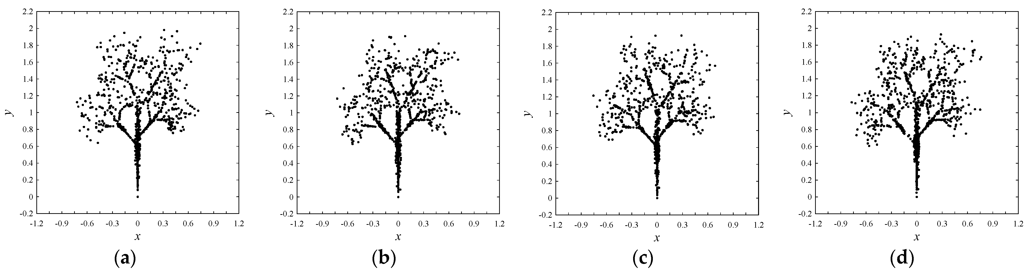
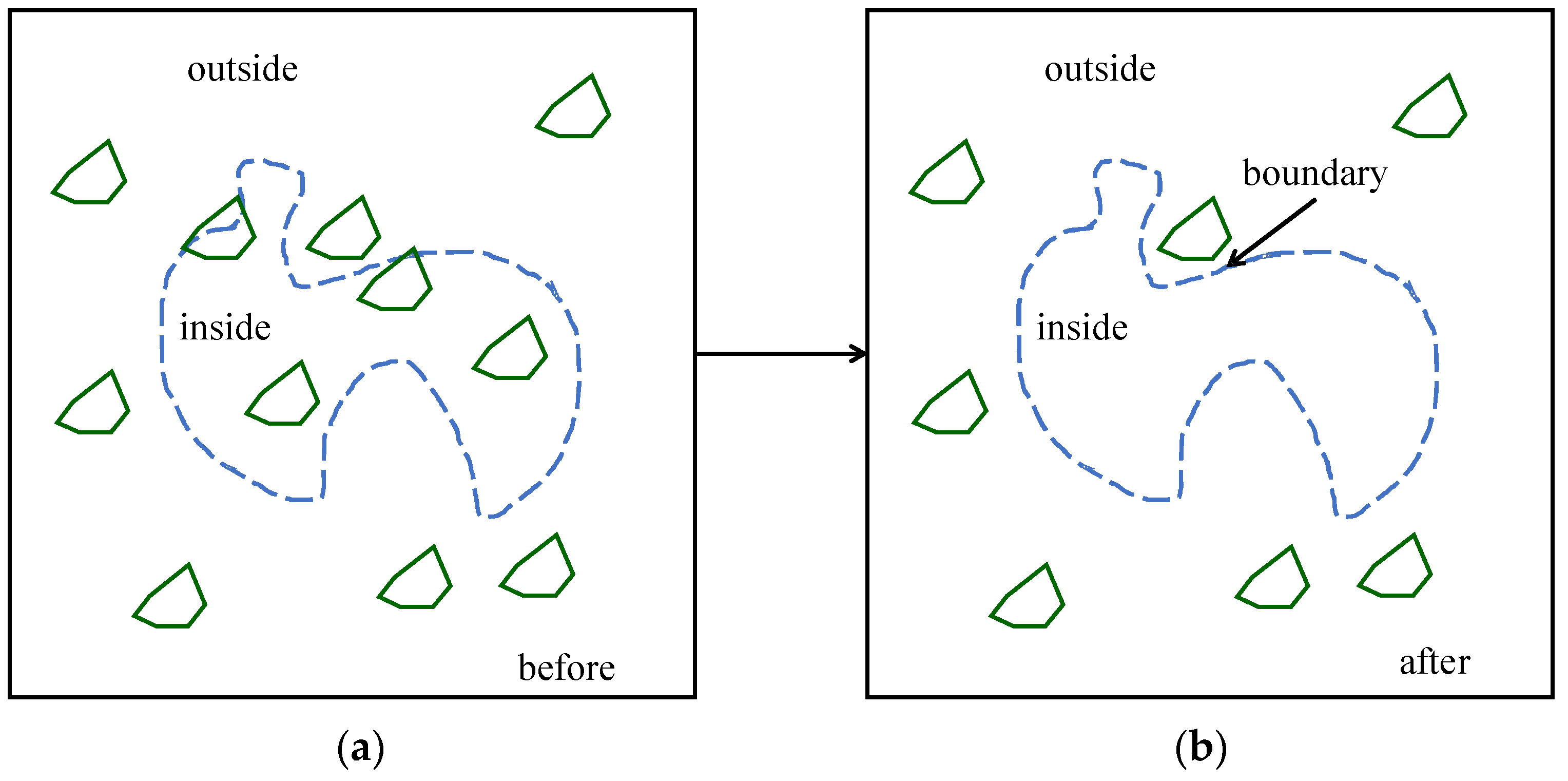
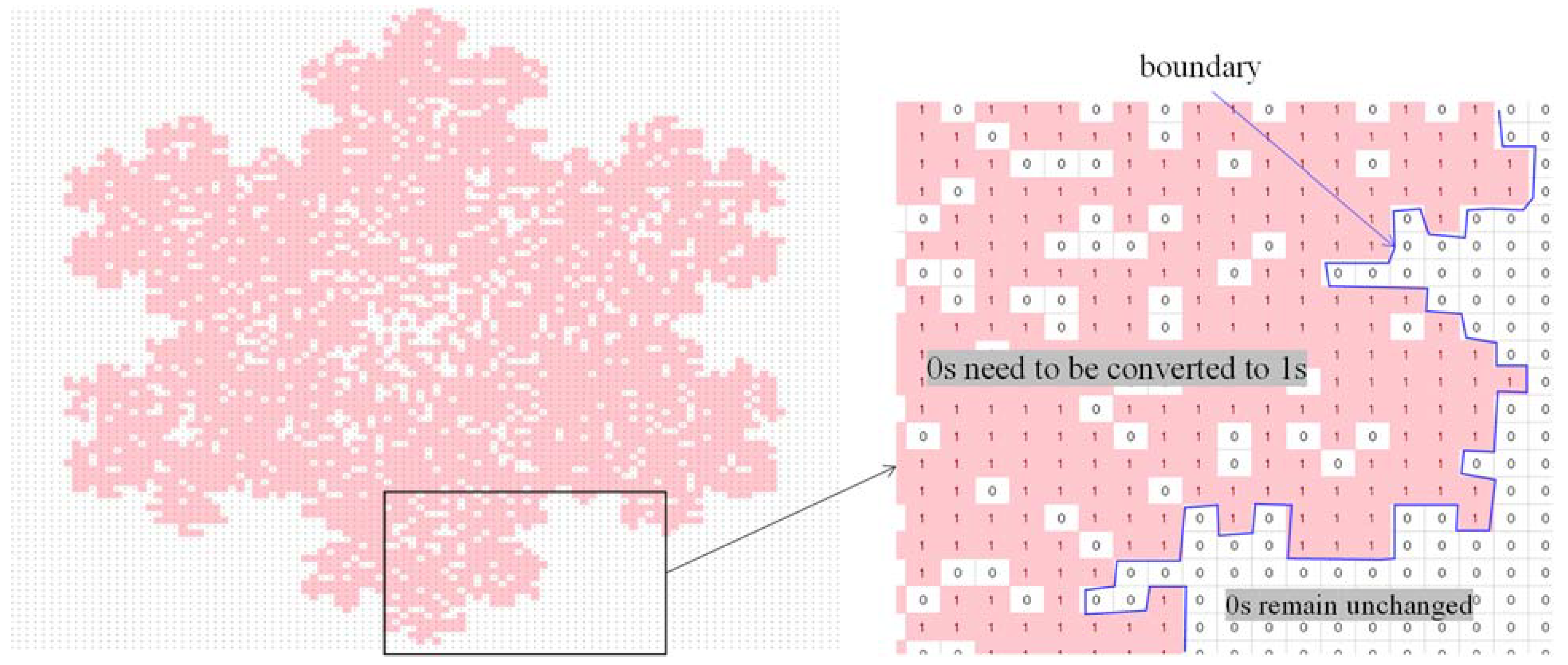
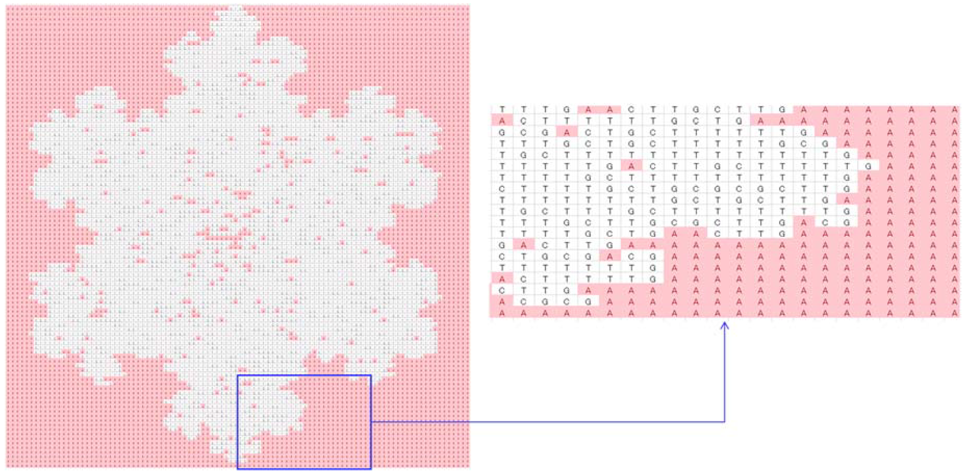
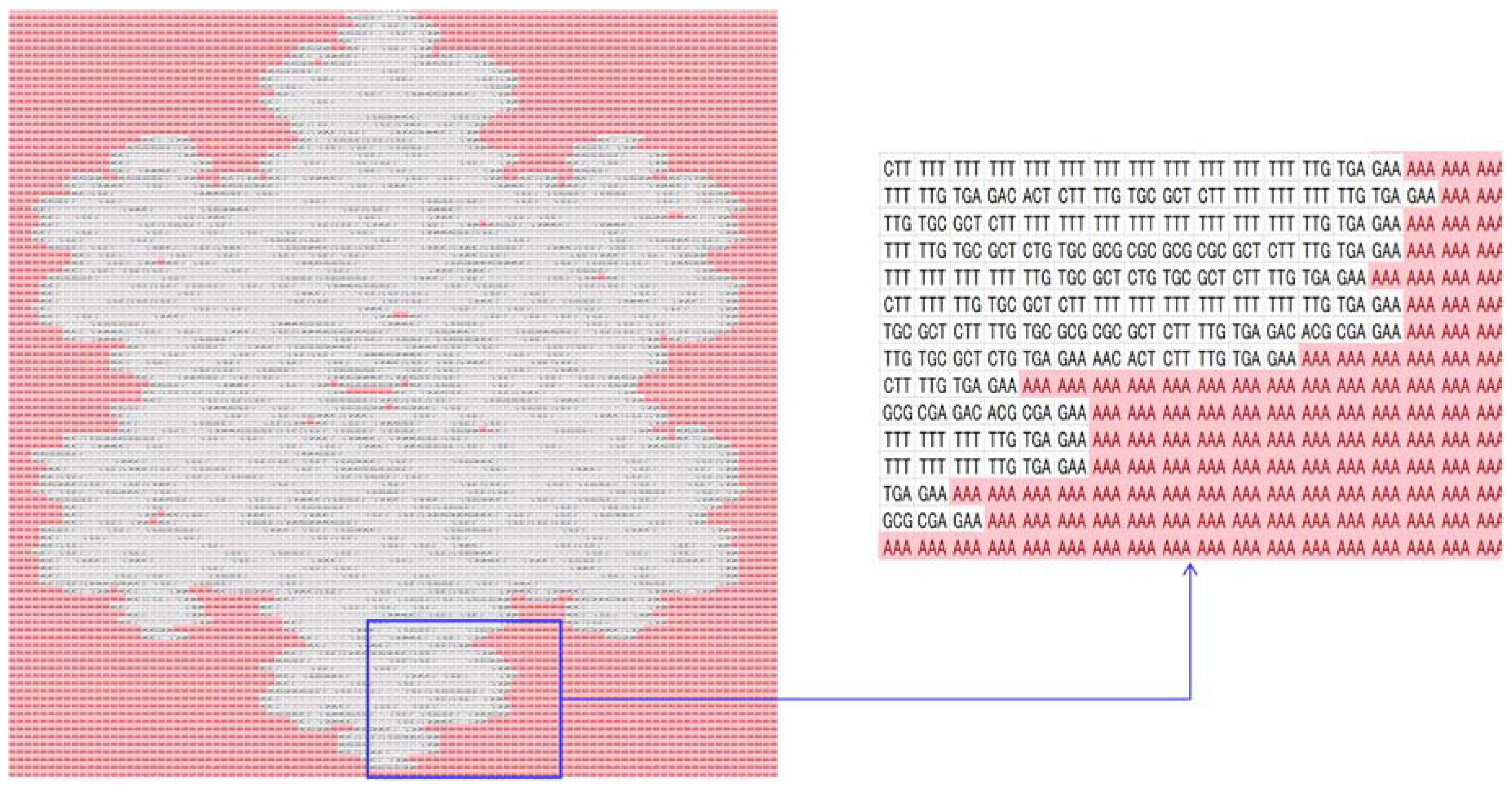
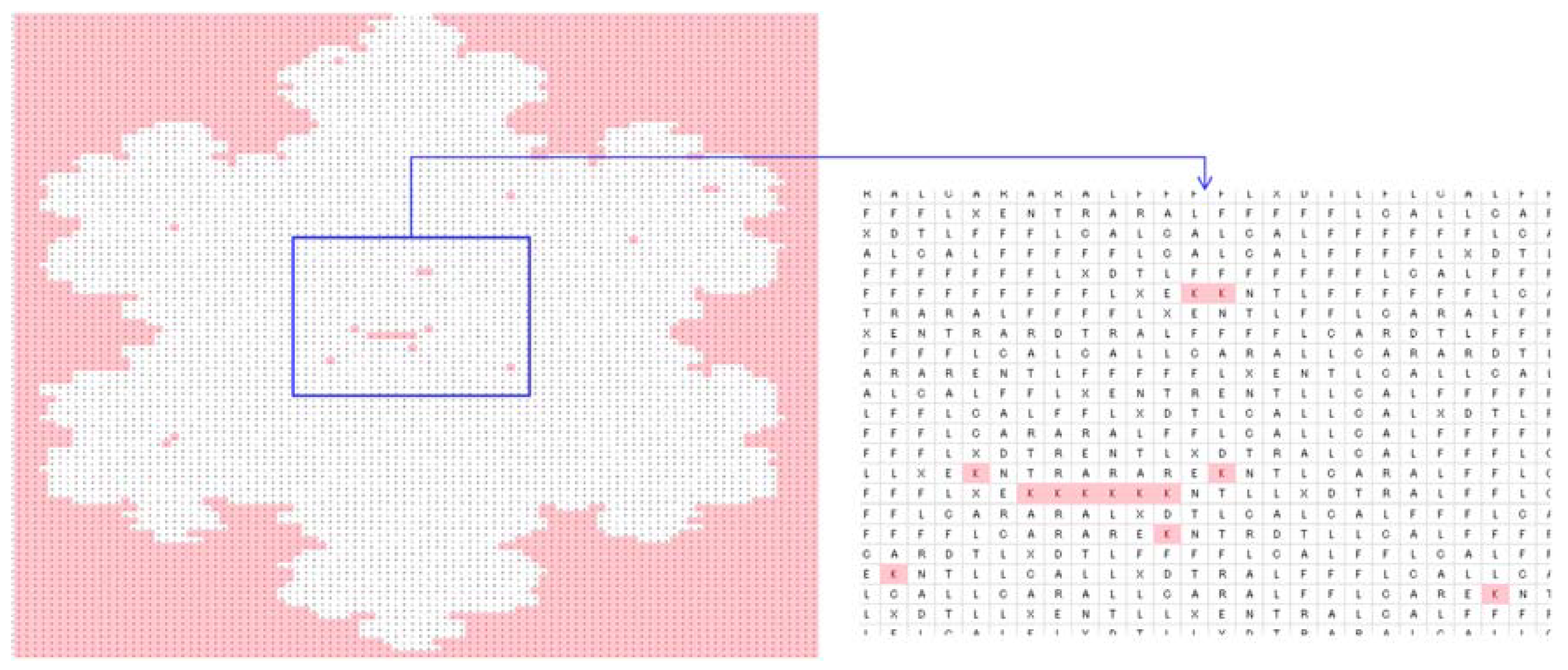
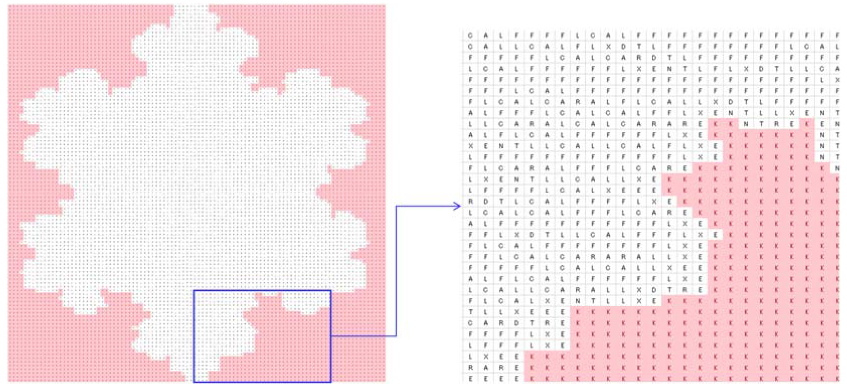
4.2. Image Processing
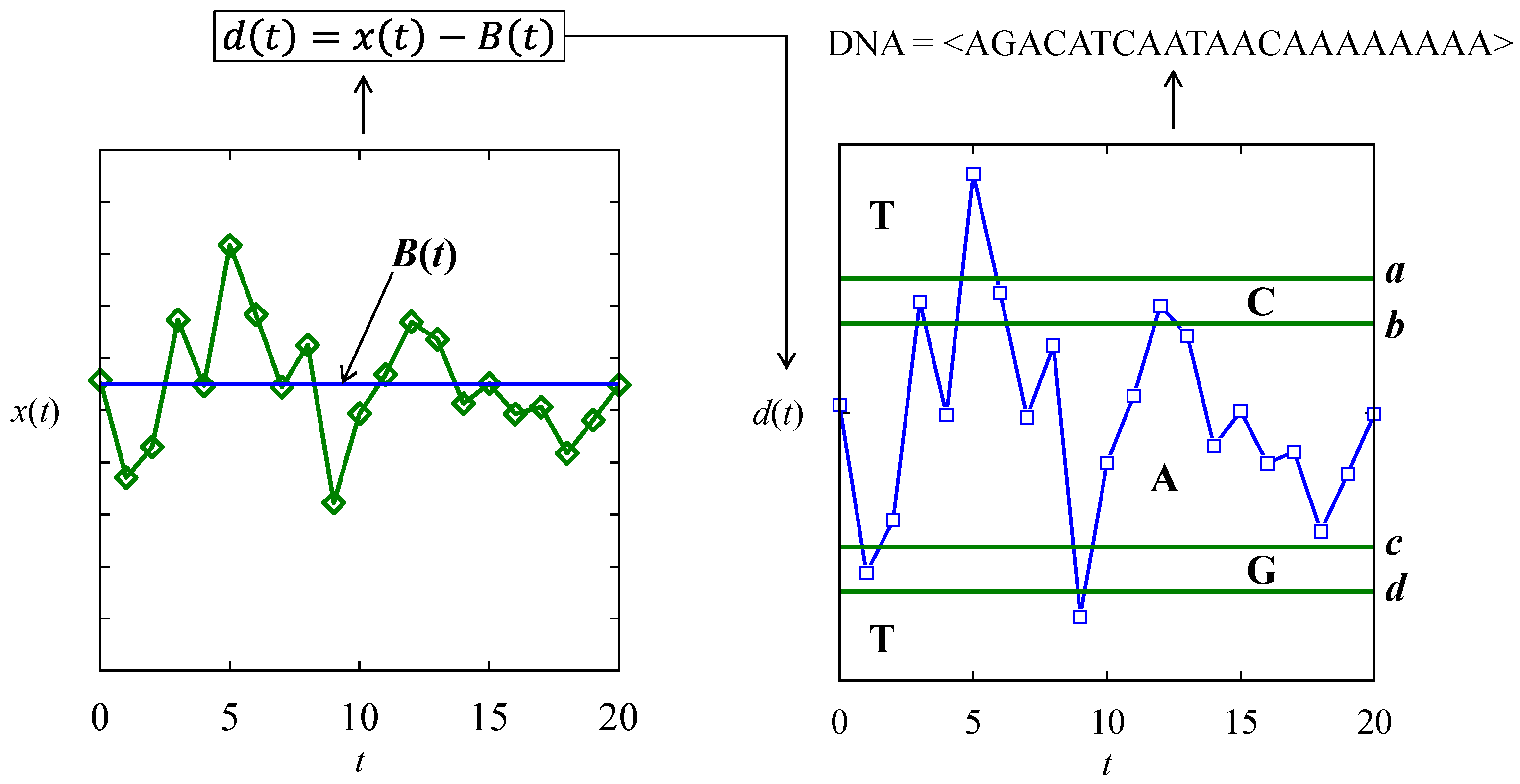
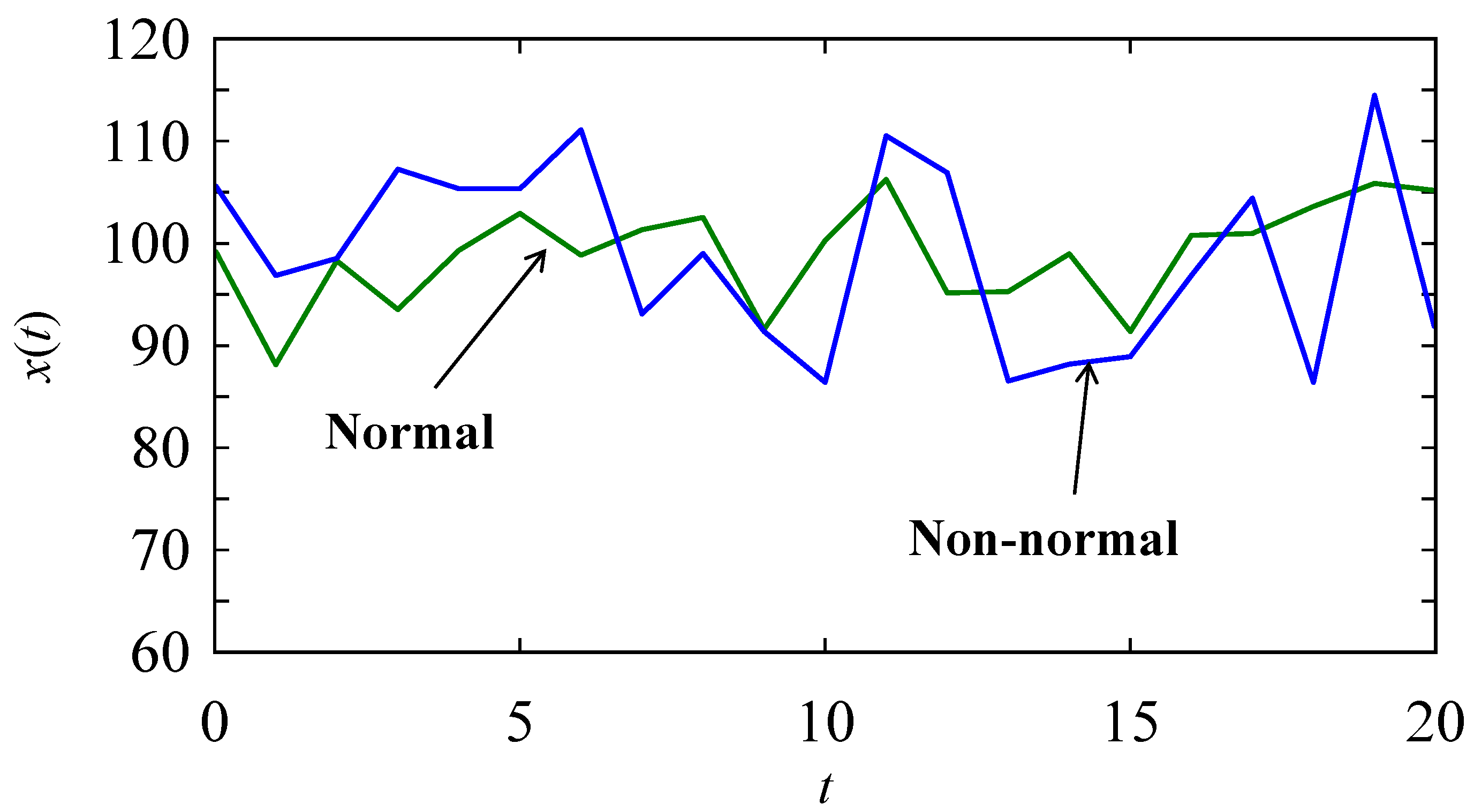
4.3. Pattern Recognition in Time Series Datasets
5. Conclusions
Author Contributions
Funding
Institutional Review Board Statement
Data Availability Statement
Conflicts of Interest
References
- Kusiak, A. Smart manufacturing. Int. J. Prod. Res. 2018, 56, 508–517. [Google Scholar] [CrossRef]
- Beckmann, B.; Giani, A.; Carbone, J.; Koudal, P.; Salvo, J.; Barkley, J. Developing the Digital Manufacturing Commons: A National Initiative for US Manufacturing Innovation. Procedia Manuf. 2016, 5, 182–194. [Google Scholar] [CrossRef]
- Dumitrescu, R.; Riemensperger, F.; Schuh, G. (Eds.) Acatech Maturity Index Smart Services: Shaping the Transformation of Businesses to Smart Service Providers (Acatech STUDY); Acatech: Munich, Germany, 2023; Available online: https://en.acatech.de/publication/acatech-maturity-index-smart-services/ (accessed on 11 December 2023). [CrossRef]
- Sharif Ullah, A.M.M. Modeling and simulation of complex manufacturing phenomena using sensor signals from the perspective of Industry 4.0. Adv. Eng. Inform. 2019, 39, 1–13. [Google Scholar] [CrossRef]
- Ghosh, A.K.; Ullah, A.M.M.S.; Teti, R.; Kubo, A. Developing sensor signal-based digital twins for intelligent machine tools. J. Ind. Inf. Integr. 2021, 24, 100242. [Google Scholar] [CrossRef]
- Byrne, G.; Dimitrov, D.; Monostori, L.; Teti, R.; van Houten, F.; Wertheim, R. Biologicalisation: Biological transformation in manufacturing. CIRP J. Manuf. Sci. Technol. 2018, 21, 1–32. [Google Scholar] [CrossRef]
- Wegener, K.; Damm, O.; Harst, S.; Ihlenfeldt, S.; Monostori, L.; Teti, R.; Wertheim, R.; Byrne, G. Biologicalisation in manufacturing—Current state and future trends. CIRP Ann. 2023, 72, 781–807. [Google Scholar] [CrossRef]
- Holland, J.H. Genetic Algorithms and Adaptation. In Adaptive Control of Ill-Defined Systems; Selfridge, O.G., Rissland, E.L., Arbib, M.A., Eds.; Springer: New York, NY, USA, 1984; pp. 317–333. [Google Scholar]
- Koza, J.R. Genetic Programming: On the Programming of Computers by Means of Natural Selection; The MIT Press: Cambridge, MA, USA, 1992. [Google Scholar]
- Affenzeller, M.; Winkler, S.; Wagner, S.; Beham, A. Genetic Algorithms and Genetic Programming: Modern Concepts and Practical Applications; Chapman & Hall/CRC: Boca Raton, FL, USA, 2009. [Google Scholar]
- Pickover, C.A. Artificial Intelligence: An Illustrated History: From Medieval Robots to Neural Networks; Sterling: New York, NY, USA, 2019. [Google Scholar]
- Wang, J.; Kusiak, A. (Eds.) Computational Intelligence in Manufacturing: Handbook; CRC Press: Boca Raton, FL, USA, 2000. [Google Scholar]
- Teti, R.; D’Addona, D.M.; Segreto, T. Microbial-based cutting fluids as bio-integration manufacturing solution for green and sustainable machining. CIRP J. Manuf. Sci. Technol. 2021, 32, 16–25. [Google Scholar] [CrossRef]
- Balkenius, C.; Johansson, B.; Tjøstheim, T.A. Elements of Cognition for General Intelligence. In Artificial General Intelligence; Hammer, P., Alirezaie, M., Strannegård, C., Eds.; Springer Nature: Cham, Switzerland, 2023; pp. 11–20. [Google Scholar]
- Voss, P. Essentials of General Intelligence. In Artificial General Intelligence; Goertzel, B., Pennachin, C., Eds.; Springer: Berlin/Heidelberg, Germany, 2007; pp. 131–157. [Google Scholar]
- Ullah, A.S. What is knowledge in Industry 4.0? Eng. Rep. 2020, 2, e12217. [Google Scholar] [CrossRef]
- Ueda, K. A concept for bionic manufacturing systems based on DNA-type information. In Human Aspects in Computer Integrated Manufacturing; Olling, G.J., Kimura, F., Eds.; Elsevier: Amsterdam, The Netherlands, 1992; pp. 853–863. [Google Scholar] [CrossRef]
- Ueda, K. Intelligent Manufacturing Systems: From Knowledge-base to Emergence-type. J. Jpn. Soc. Precis. Eng. 1993, 59, 1755–1760. [Google Scholar] [CrossRef]
- Okino, N. Bionic Manufacturing System. In Flexible Manufacturing Systems Past-Present-Future; Peklenik, J., Ed.; CIRP: Paris, France, 1993; pp. 73–95. [Google Scholar]
- Ueda, K. Bio-Oriented Production System (Seibutsu Shikō-Gata Seisan Shisutemu); Kogyo Chosakai Publishing: Tokyo, Japan, 1994. (In Japanese) [Google Scholar]
- Okino, N. Conception of Bionic Systems: Biological Metaphor for Systems Construction. Trans. Inst. Syst. Control Inf. Eng. 1995, 8, 381–390. [Google Scholar] [CrossRef]
- Ueda, K.; Vaario, J.; Ohkura, K. Modelling of Biological Manufacturing Systems for Dynamic Reconfiguration. CIRP Ann. 1997, 46, 343–346. [Google Scholar] [CrossRef]
- Tharumarajah, A. Comparison of the bionic, fractal and holonic manufacturing system concepts. Int. J. Comput. Integr. Manuf. 1996, 9, 217–226. [Google Scholar] [CrossRef]
- Sugimura, N.; Moriwaki, T.; Hozumi, K. A study on holonic manufacturing systems and its application to real time scheduling problems. In Advances in Production Management Systems: Perspectives and Future Challenges; Okino, N., Tamura, H., Fujii, S., Eds.; Springer: New York, NY, USA, 1998; pp. 411–422. [Google Scholar]
- Ryu, K.; Jung, M. Agent-based fractal architecture and modelling for developing distributed manufacturing systems. Int. J. Prod. Res. 2003, 41, 4233–4255. [Google Scholar] [CrossRef]
- Denkena, B.; Morke, T. Cyber-Physical and Gentelligent Systems in Manufacturing and Life Cycle: Genetics and Intelligence–Keys to Industry 4.0; Academic Press: Cambridge, MA, USA, 2017. [Google Scholar]
- Denkena, B.; Dittrich, M.-A.; Stamm, S.; Wichmann, M.; Wilmsmeier, S. Gentelligent processes in biologically inspired manufacturing. CIRP J. Manuf. Sci. Technol. 2021, 34, 105–118. [Google Scholar] [CrossRef]
- Ullah, A.M.M.S.; Yano, A.; Higuchi, M. Protein Synthesis Algorithm and a New Metaphor for Selecting Optimum Tools. JSME Int. J. Ser. C 1997, 40, 540–546. [Google Scholar] [CrossRef]
- Shuta, Y.; Ullah, A.M.M.S.; Yano, A.; Higuchi, M.; Yamaguchi, T. Grinding Wheel Design Based on the Model of Protein Synthesis. J. Jpn. Soc. Grind. Eng. 1998, 42, 418–423. (In Japanese) [Google Scholar]
- Ullah, A.M.M.S. A DNA-based computing method for solving control chart pattern recognition problems. CIRP J. Manuf. Sci. Technol. 2010, 3, 293–303. [Google Scholar] [CrossRef]
- Ullah, A.M.M.S.; D’Addona, D.; Arai, N. DNA based computing for understanding complex shapes. Biosystems 2014, 117, 40–53. [Google Scholar] [CrossRef]
- D’Addona, D.M.; Ullah, A.M.M.S.; Matarazzo, D. Tool-wear prediction and pattern-recognition using artificial neural network and DNA-based computing. J. Intell. Manuf. 2017, 28, 1285–1301. [Google Scholar] [CrossRef]
- Iwadate, K.; Ullah, S. Determining Outer Boundary of a Complex Point-Cloud using DNA Based Computing. Trans. Jpn. Soc. Evol. Comput. 2020, 11, 1–8. (In Japanese) [Google Scholar] [CrossRef]
- Ghosh, A.K.; Ullah, A.S.; Kubo, A.; Akamatsu, T.; D’Addona, D.M. Machining Phenomenon Twin Construction for Industry 4.0: A Case of Surface Roughness. J. Manuf. Mater. Process. 2020, 4, 11. [Google Scholar] [CrossRef]
- Kubo, A.; Teti, R.; Ullah, A.S.; Iwadate, K.; Segreto, T. Determining Surface Topography of a Dressed Grinding Wheel Using Bio-Inspired DNA-Based Computing. Materials 2021, 14, 1899. [Google Scholar] [CrossRef] [PubMed]
- Crick, F. Central dogma of molecular biology. Nature 1970, 227, 561–563. [Google Scholar] [CrossRef] [PubMed]
- Cobb, M. 60 years ago, Francis Crick changed the logic of biology. PLoS Biol. 2017, 15, e2003243. [Google Scholar] [CrossRef]
- Alberts, B.; Johnson, A.; Lewis, J.; Raff, M.; Roberts, K.; Walter, P. Molecular Biology of the Cell, 4th ed.; Garland Science: New York, NY, USA, 2002. [Google Scholar]
- Shannon, C.E. A mathematical theory of communication. Bell Syst. Tech. J. 1948, 27, 379–423. [Google Scholar] [CrossRef]
- Barnsley, M.F.; Demko, S. Iterated Function Systems and the Global Construction of Fractals. Proc. R. Soc. London. Ser. A Math. Phys. Sci. 1985, 399, 243–275. [Google Scholar] [CrossRef]
- Sharif Ullah, A.M.M.; Sato, Y.; Kubo, A.; Tamaki, J. Design for Manufacturing of IFS Fractals from the Perspective of Barnsley’s Fern-leaf. Comput. Aided Des. Appl. 2015, 12, 241–255. [Google Scholar] [CrossRef]


| DNA | mRNA (Codon) | tRNA (Anti-Codon) |
|---|---|---|
| A | U | A |
| C | G | C |
| G | C | G |
| T | A | U |
| Nucleic acid symbols | ||
| No | Three-Letter DNA Bases (Codons $) | Amino Acids (Single-Letter Symbols) |
|---|---|---|
| 1 | ATT, ATC, ATA | Isoleucine (I) |
| 2 | CTT, CTC, CTA, CTG, TTA, TTG | Leucine (L) |
| 3 | GTT, GTC, GTA, GTG | Valine (V) |
| 4 | TTT, TTC | Phenylalanine (F) |
| 5 | ATG | Methionine (M) |
| 6 | TGT, TGC | Cysteine (C) |
| 7 | GCT, GCC, GCA, GCG | Alanine (A) |
| 8 | GGT, GGC, GGA, GGG | Glycine (G) |
| 9 | CCT, CCC, CCA, CCG | Proline (P) |
| 10 | ACT, ACC, ACA, ACG | Threonine (T) |
| 11 | TCT, TCC, TCA, TCG, AGT, AGC | Serine (S) |
| 12 | TAT, TAC | Tyrosine (Y) |
| 13 | TGG | Tryptophan (W) |
| 14 | CAA, CAG | Glutamine (Q) |
| 15 | AAT, AAC | Asparagine (N) |
| 16 | CAT, CAC | Histidine (H) |
| 17 | GAA, GAG | Glutamic acid (E) |
| 18 | GAT, GAC | Aspartic acid (D) |
| 19 | AAA, AAG | Lysine (K) |
| 20 | CGT, CGC, CGA, CGG, AGA, AGG | Arginine (R) |
| 21 | TAA, TAG, TGA | None (X %) |
| Items | Settings |
|---|---|
| Problem relevant information | A (100 × 100) binary array of the tree |
| DNA-forming rules | 00 = A, 01 = C, 10 = G, 11 = T, continuous reading frame; truncation/addition: truncation |
| Protein-forming rules | As described in Section 3 |
| Rules | |
|---|---|
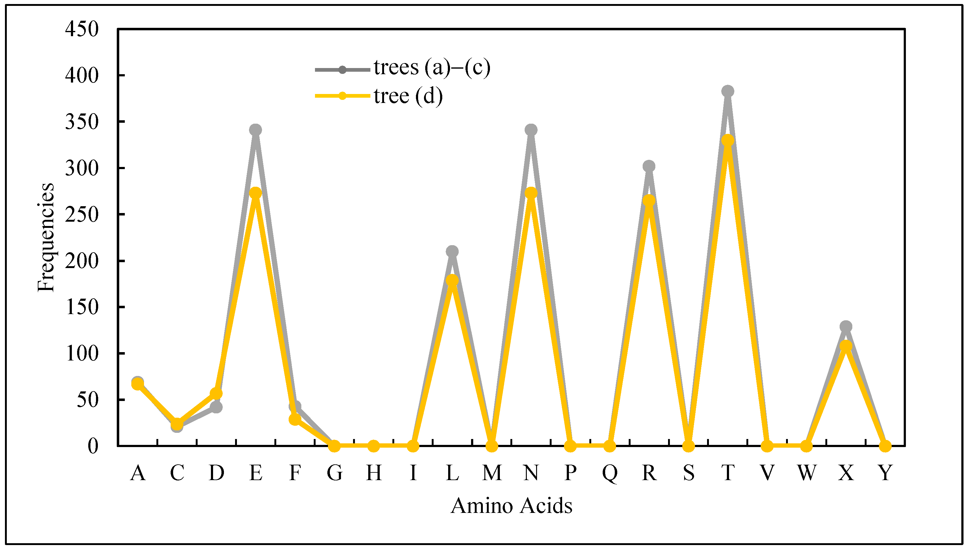
| Zero-frequency amino acids | G, H, I, M, P, Q, S, V, W, and Y |
| Equal-frequency amino acids | E and N (341 for trees Figure 4a–c and 273 for Figure 4d) |
| Special frequencies | Summation of frequencies of D and N is equal to the frequency of T, i.e., (fr(D) + fr(N) = fr(T) = 383 for trees Figure 4a–c and 330 for the tree in Figure 4d) |
| The least frequent amino acid other than the zero-frequency ones | C |
| List of amino acids in the ascending order of frequencies | fr(A) < fr(X) < fr(L) < fr(R) < fr(E) < fr(N) < fr(T) |
| Items | Settings |
|---|---|
| Baseline and thresholds | B(t) = 100, a = 10, b = 5, c = −5, and d = 10 for all three DNA arrays |
| mRNA-forming rules | Cascading rule among the three DNA: DNA1,…,DNA3 mRNA = <…codon(i) = DNA1(i)DNA2(i)DNA3(i)…> |
| Protein-forming rules | As described in Section 3 |
| No | Protein Arrays (Normal) | Proteins Arrays (Not Normal) | Entropy [dna] (Normal) | Entropy [dna] (Non-Normal) | Problem-Solving Rule Holds |
|---|---|---|---|---|---|
| 1 | KKKPFKKKKKPKKGKKPKFKK | KFKGPFKFKKGFKKGPFGFKK | 0.640 | 0.910 | yes |
| 2 | KGKKKKKKKKKKKKKPKKKGP | FKKGFPGGGKKPKFKFPKGKK | 0.446 | 0.937 | yes |
| 3 | PKGKKGKPPPPGKFKKKKKKK | PGKKKFPFFFFFKFKFFFFFP | 0.782 | 0.782 | yes |
| 4 | PKKPGKPKFFFKKKKPPKKKP | FFGKFKGKKKGFKFGPFKGPK | 0.808 | 0.931 | yes |
| 5 | KGKPKPKPKKKKKGKPKKKGK | KPFGKPKFFPFFKGFGGPPKF | 0.623 | 0.985 | yes |
| 6 | PKGGKFGKKKKKKKKGKKKKK | PPFKKGKGFFFKFFFGGGKKF | 0.610 | 0.931 | yes |
| 7 | KKKGKKKKKKKPKGKKKKKKP | FKKGKFKKPFKGFKFKGFKFF | 0.446 | 0.832 | yes |
| 8 | KKKKPKFPKFKKKKKKKKKKK | GPKFFKKFFPKGPFGKFGPKP | 0.446 | 0.991 | yes |
| 9 | GKKKKFPPKKKPFKPKGPPPK | FPKGKKFFFKKFPGGKGPGKF | 0.842 | 0.969 | yes |
| 10 | PFKKGKKPKKKFKKPKKKKKK | GKFGFKKFKFPFFPFGGFKKK | 0.640 | 0.919 | yes |
| 11 | KKFKKKKPKKKKKPKKGKKKK | FPFFKGFGKFGGFFGKGKPGK | 0.494 | 0.936 | yes |
| 12 | KKKFKKPKKKFFKPKKKKKKK | KFGKFGPKFFGKKPGFKGGGK | 0.512 | 0.936 | yes |
| 13 | KGKKKKKPKKKKKKKKKKKKK | FFKPGFGPGKGKGPKFPPFFF | 0.274 | 0.985 | yes |
| 14 | KKKKKPPKKKKKKGGKGGKPP | GGKFKPFKKFGKKKFKFFFKK | 0.670 | 0.824 | yes |
| 15 | KKKKKPGKKKKKKKKKPKKPK | FKKFGFFKFFFGGGGFGGGPF | 0.428 | 0.832 | yes |
| 16 | PGPKPKKPPKPKKKKKKKKKK | PKGGPPPFFFKFFPFFGPKPK | 0.558 | 0.957 | yes |
| 17 | KGKGKPGKKFKKKKPKKKKKP | FFFFKKPKGKKFKKKPPFFKK | 0.701 | 0.824 | yes |
| 18 | KGKGKKGKKKKFGKPKPKGKK | PKPPFKKKPKFKKFKKFFFPF | 0.727 | 0.773 | yes |
| 19 | GKPKKKKKPFKPPKPKKKKKG | FGPFFKFGFFKKKGKGKGFGP | 0.727 | 0.942 | yes |
| 20 | KPKGKGKKKGKKGKGKPKKGK | GPFGKGKGGFFFFGPGPPGKP | 0.634 | 0.959 | yes |
Disclaimer/Publisher’s Note: The statements, opinions and data contained in all publications are solely those of the individual author(s) and contributor(s) and not of MDPI and/or the editor(s). MDPI and/or the editor(s) disclaim responsibility for any injury to people or property resulting from any ideas, methods, instructions or products referred to in the content. |
© 2023 by the authors. Licensee MDPI, Basel, Switzerland. This article is an open access article distributed under the terms and conditions of the Creative Commons Attribution (CC BY) license (https://creativecommons.org/licenses/by/4.0/).
Share and Cite
Ura, S.; Zaman, L. Biologicalization of Smart Manufacturing Using DNA-Based Computing. Biomimetics 2023, 8, 620. https://doi.org/10.3390/biomimetics8080620
Ura S, Zaman L. Biologicalization of Smart Manufacturing Using DNA-Based Computing. Biomimetics. 2023; 8(8):620. https://doi.org/10.3390/biomimetics8080620
Chicago/Turabian StyleUra, Sharifu, and Lubna Zaman. 2023. "Biologicalization of Smart Manufacturing Using DNA-Based Computing" Biomimetics 8, no. 8: 620. https://doi.org/10.3390/biomimetics8080620