Article

OOBO: A New Metaheuristic Algorithm for Solving Optimization Problems

1
Department of Mathematics, Faculty of Science, University of Hradec Králové, 50003 Hradec Králové, Czech Republic
2
Department of Electrical and Software Engineering, University of Calgary, Calgary, AB T2N 1N4, Canada
*
Author to whom correspondence should be addressed.
Biomimetics 2023, 8(6), 468; https://doi.org/10.3390/biomimetics8060468
Submission received: 24 August 2023 / Revised: 23 September 2023 / Accepted: 27 September 2023 / Published: 1 October 2023
(This article belongs to the Special Issue Bioinspired Algorithms)

Abstract

:
This study proposes the One-to-One-Based Optimizer (OOBO), a new optimization technique for solving optimization problems in various scientific areas. The key idea in designing the suggested OOBO is to effectively use the knowledge of all members in the process of updating the algorithm population while preventing the algorithm from relying on specific members of the population. We use a one-to-one correspondence between the two sets of population members and the members selected as guides to increase the involvement of all population members in the update process. Each population member is chosen just once as a guide and is only utilized to update another member of the population in this one-to-one interaction. The proposed OOBO’s performance in optimization is evaluated with fifty-two objective functions, encompassing unimodal, high-dimensional multimodal, and fixed-dimensional multimodal types, and the CEC 2017 test suite. The optimization results highlight the remarkable capacity of OOBO to strike a balance between exploration and exploitation within the problem-solving space during the search process. The quality of the optimization results achieved using the proposed OOBO is evaluated by comparing them to eight well-known algorithms. The simulation findings show that OOBO outperforms the other algorithms in addressing optimization problems and can give more acceptable quasi-optimal solutions. Also, the implementation of OOBO in six engineering problems shows the effectiveness of the proposed approach in solving real-world optimization applications.

1. Introduction

The term “optimization” refers to obtaining the optimal solution out of all available solutions to a problem [1]. Optimization appears widely in real-world issues. For example, the goal of engineers is to design a product with the best performance, traders seek to maximize profits from their transactions, and investors try to minimize investment risk, etc. [2]. These types of problems must be modeled mathematically and then optimized using the appropriate method. Each optimization problem is composed of three parts: (a) decision variables, (b) constraints, and (c) objective functions that can be modeled using Equations (1)–(4).
Minimize / Maximize :   f x ,   x = x 1 , x 2 ,   , x m
Subject to:
g i x < 0 ,     i = 1,2 ,   ,   p ,
h k x = 0 ,     k = 1,2 ,   , q ,
l b j x j u b j ,     j = 1,2 ,   , m ,
where m is the number of problem variables, x = ( x 1 , x 2 , , x m ) is the vector of problem variables, f ( x ) is the values of the objective function for problem variables, g i is the i th inequality constraint, p is the total number of inequality constraints, h k is the k th equality constraint, q is the total number of equality constraints, and l b j and u b j are the lower and upper bounds of the j th problem variable x j , respectively.
Problem-solving techniques in the study of optimization problems fall into two categories. The first category consists of “exact algorithms” that find optimal solutions to these problems and guarantee the optimality of these solutions. The second category consists of “approximate algorithms,” which are usually designed to solve optimization problems that exact methods are unable to solve [3]. In contrast to exact algorithms, approximate algorithms are able to generate appropriate quality solutions for many optimization problems in a reasonable period of time. However, the important issue with approximate algorithms is that there is no assurance that the problem’s global optimal solution will be found [4]. As a result, solutions derived from approximation approaches are referred to as quasi-optimal [5]. A quasi-optimal solution should be as near to the global optimum as feasible.
Random-based optimization algorithms are among the most extensively utilized approximate algorithms in the solution of optimization problems. Optimization algorithms can give acceptable quasi-optimal solutions for objective functions by employing random operators and random scanning of the optimization problem’s search space [6]. The proximity of their offered quasi-optimal solution to the global optimum is the key criterion of optimization algorithms’ superiority over one another. Scholars created numerous optimization techniques in this respect with the goal of finding quasi-optimal solutions that are closer to the global optimum. These random-based optimization algorithms are used in solving combinatorial optimization problems.
The main question that arises is whether there is still a need to design new optimizers, given that numerous optimization algorithms have been produced. According to the No Free Lunch (NFL) theorem [7], even if an optimization method is very good at solving a certain set of optimization problems, there is no guarantee that it will be an effective optimizer for other optimization problems. As a result, it is impossible to declare that a specific method is the best optimizer for all optimization challenges. The NFL theorem has prompted researchers to design new optimizers to handle optimization issues in a variety of fields [8]. This motivated the authors of this study to develop a novel optimization approach to optimizing real-world engineering problems that are both effective and gradient-free.
The novelty and innovation of this paper are in developing a novel population-based optimization method called the One-to-One-Based Optimizer (OOBO) to handle diverse optimization problems. The main contributions of this paper are as follows:
  • The key idea behind the suggested OOBO algorithm is the effective use of different members of the population and not relying on specific members during the population updating process.
  • The suggested OOBO algorithm’s theory is discussed, and its mathematical model for applications in solving optimization problems is offered.
  • OOBO’s ability to provide appropriate solutions is evaluated with fifty-two distinct objective functions.
  • The effectiveness of OOBO in solving real-world applications is tested on four engineering design problems.
  • The performance of OOBO is compared with eight well-known algorithms to assess its quality and ability.
The proposed OOBO approach has advantages, such as simple concepts, simple equations, and convenient implementation. The main advantage of OOBO is that it does not have any control parameters; therefore, the proposed approach does not need to adjust the parameters (of course, it should be mentioned, except for the population size, i.e., N and the maximum number of iterations of the algorithm, i.e., T, which are present in all metaheuristic algorithms due to the nature of population-based metaheuristic algorithms). In addition, the optimization process in the proposed OOBO ensures that a member of the population is employed solely to guide a member of the population in each iteration of the algorithm. Therefore, all members participate in guiding the OOBO population.
The rest of the paper is as follows: A literature review is presented in Section 2. Section 3 introduces the suggested OOBO algorithm. Section 4 contains simulation studies and results. The evaluation of OOBO for optimizing four real-life problems is presented in Section 5. Finally, conclusions and several recommendations for further research are stated in Section 6.

2. Literature Review

Optimization algorithms are classified into five types, based on their primary design concepts: (a) swarm-based, (b) physics-based, (c) evolutionary-based, (d) human-based, and (e) game-based approaches.
Swarm-based optimization methods were inspired by various natural phenomena and natural behaviors of living organisms in nature. Particle swarm optimization (PSO) is among the oldest and most extensively used algorithms in this category, and it was designed based on natural fish and bird behaviors [9]. Ant colony optimization (ACO) is another swarm-based technique that is focused on simulating ants’ behavior as they travel between nests and food sources, as well as the placement of pheromones in their paths. The presence of more pheromones in a path indicates that the path is closer to the food source [10]. The bat algorithm (BA) is designed by imitating the activity of bats’ sound systems in locating prey, obstacles, and nests [11]. Grey wolf optimization is a nature-based technique that models the hierarchical structure of grey wolves’ social behavior during hunting [12]. Some of the other swarm-based optimization algorithms are green anaconda optimization (GOA) [13], the spotted hyena optimizer (SHO) [14], northern goshawk optimization (NGO) [15], the orca predation algorithm (OPA) [16], the artificial fish-swarm algorithm (AFSA) [17], the reptile search algorithm (RSA) [18], the firefly algorithm (FA) [19], the grasshopper optimization algorithm (GOA) [20], dolphin partner optimization (DPO) [21], the whale optimization algorithm (WOA) [22], the hunting search (HS) [23], moth–flame optimization (MFO) [24], the seagull optimization algorithm (SOA) [25], the subtraction-average-based optimizer (SABO) [26], the remora optimization algorithm (ROA) [27], the marine predators algorithm (MPA) [28], the artificial hummingbird algorithm (AHA) [29], red fox optimization (RFO) [30], the tunicate swarm algorithm (TSA) [31], the pelican optimization algorithm (POA) [32], the cat- and mouse-based optimizer (CMBO) [33], the selecting-some-variables-to-update-based algorithm (SSVUBA) [34], the good, the bad, and the ugly optimizer (GBUO) [35], the group mean-based optimizer (GMBO) [36], and the snake optimizer (SO) [37].
Physics-based optimization algorithms are produced by drawing inspiration from numerous physical occurrences and using a variety of its rules. Simulated annealing (SA) is one of the methods in this group that originates from the process of refrigerating molten metals. In the refrigeration process, a very high-temperature molten metal is gradually cooled [38]. The gravitational search algorithm (GSA) is designed by modeling the force of gravity and Newton’s laws of motion in an artificial system in which masses apply force to each other at different distances and move in this system according to such laws [39]. Some of the other physics-based optimization algorithms are the galaxy-based search algorithm (GbSA) [40], the small world optimization algorithm (SWOA) [41], Henry gas solubility optimization (HGSO) [42], central force optimization (CFO) [43], ray optimization (RO) [44], the flow regime algorithm (FRA) [45], curved space optimization (CSO) [46], the billiards-inspired optimization algorithm (BOA) [47], and nuclear reaction optimization (NRO) [48].
Evolutionary-based optimization algorithms are based on the simulation of biological evolution and the theory of natural selection. This category includes the genetic algorithm (GA), one of the earliest approximation optimizers. The GA was developed by modeling the reproductive process according to Darwin’s theory of evolution using three operators: (a) selection, (b) crossover, and (c) mutation [49]. Some of the other evolutionary-based optimization algorithms are the biogeography-based optimizer (BBO) [50], the memetic algorithm (MA) [51], evolutionary programming (EP) [52], the drawer algorithm (DA) [53], evolution strategy (ES) [54], differential evolution (DE) [55], and genetic programming (GP) [56].
Human-based optimization algorithms are developed based on modeling human behavior. Teaching–learning-based optimization (TLBO) is among the most employed human-based algorithms and models the educational process in the classroom between teachers and students. In the TLBO, the educational process is implemented in two phases: (a) a teaching phase in which the teacher shares knowledge with the students and (b) a learner phase in which the students share knowledge with each other [57]. Some of the other human-based optimization algorithms are the mother optimization algorithm (MOA) [58], the exchange market algorithm (EMA) [59], the group counseling optimizer (GCO) [60], the teamwork optimization algorithm (TOA) [6], dual-population social group optimization (DPSGO) [61], and the election-based optimization algorithm (EBOA) [6].
Game-based optimization algorithms originate from the rules of various groups or individual games. The volleyball premier league (VPL) algorithm is based on modeling the interaction and competition among volleyball teams during a season and the coaching process during a match [62]. Some of the other game-based optimization algorithms are football game-based optimization (FGBO) [63], ring toss game-based optimization (RTGBO) [64], the golf optimization algorithm (GOA) [65], and shell game optimization (SGO) [66].
Some other recently proposed metaheuristic algorithms are monarch butterfly optimization (MBO) [67], the slime mold algorithm (SMA) [68], the moth search algorithm (MSA) [69], the Hunger Games search (HGS) [70], the Runge Kutta method (RUN) [71], the colony predation algorithm (CPA) [72], the weighted mean of vectors (INFO) [73], Harris Hawks optimization (HHO) [74], and the Rime optimization algorithm (RIME) [75].

3. One-to-One Based Optimizer

In this section, the proposed OOBO algorithm is described, and its mathematical modeling is presented. OOBO is a population-based metaheuristic algorithm that can provide effective solutions to optimization problems in an iteration-based process using a population search power in the problem-solving space.

3.1. Basis of the Algorithm

The basis of OOBO is that, first, several feasible solutions are generated based on the constraints of the problem. Then, in each iteration, the position of these solutions in the search space is updated, employing the algorithm’s main idea. Excessive reliance on specific population members in the update process prevents accurate scanning of the problem’s search space. This can lead to the convergence of the algorithm towards local optimal areas. The main idea in designing the proposed OOBO algorithm, while preventing it from relying too much on specific members of the population, such as best, worst, and mean members, is the effective use of information on all population members in the process of updating the algorithm population. Therefore, in this process of updating, the following items are considered: (a) the non-reliance of population updates on its specific members; (b) the involvement of all members in the updating process; and (c) each population member is employed in a one-to-one correspondence to guide another member in the search space.

3.2. Algorithm Initialization

In the OOBO algorithm, each population member is a proposed solution to the given problem as values for the decision variables, depending on its location in the search space. As a result, in OOBO, each population member is mathematically represented by a vector with the same number of elements as the number of decision variables. A population member can be represented using
X i = x i , 1 ,   ,   x i , d ,   ,   x i , m ,   i = 1 ,   ,   N .
To generate the initial population of OOBO, population members are randomly positioned in the search space utilizing
x i , d = l b d + r a n d ( ) · u b d l b d ,   d = 1 ,   , m ,
where X i is the i th population member (that is, the proposed solution), x i , d is its d th dimension (that is, the proposed value for the d th variable), rand() is a function generating a random uniform number from the interval 0 ,   1 , and N is the size of the population.
In OOBO, the algorithm population is represented using a matrix according to
X = X 1 X i X N = x 1,1 x 1 , d x 1 , m   x i , 1 x i , d x i , m x N , 1 x N , d x N , m N × m .
The optimization problem’s objective function can be assessed based on each population member, which is a proposed solution. Thus, different values for the objective function are acquired in each iteration equal to the number of population members, which can be mathematically described by means of
F = f 1 f i f N N × 1 = f ( X 1 ) f ( X i ) f ( X N ) N × 1 ,
where F is the objective function vector and f i is the objective function value for the i th proposed solution.

3.3. Mathematical Modeling of OOBO

At this stage of mathematical modeling for the OOBO algorithm, the population members’ positions must be updated in the search space. The main difference between metaheuristic algorithms is in how to update the position of population members. One of the things that can be seen in many metaheuristic algorithms is that the population update process is strongly dependent on the best member. This may lead to a decrease in the algorithm’s exploration ability to provide the global search in the problem-solving space and then get stuck in the local optimum. In fact, moving the population towards the best member can cause convergence to inappropriate local solutions, especially in complex optimization problems. Meanwhile, in the design of OOBO, the dependence of the population update process on the best member has been prevented. Hence, by moving the population of the algorithm to different areas in the search space, the exploration power of OOBO can be increased to provide the global search. The main idea of OOBO for this process is that all members of the population should participate in population updating. Therefore, each population member is selected only once and randomly to guide a different member of the population in the search space. We can mathematically describe this idea using an N -tuple with the following properties: (a) each member is randomly selected from the positive integers from 1 to N ; (b) there are no duplicate members among its members; and (c) no member has a value equal to its position in this N -tuple.
To model a one-to-one correspondence, the member position number in the population matrix is used. The random process of forming the set K as “the set of the positions of guiding members” is modeled by
K = k 1 , , k l , , k N P N ¯ ;   l N ¯ : k l l ,
where N ¯ = 1 ,   ,   N , P N ¯ is the set of all permutations of the set N ¯ , and k l is the l th element of the vector K .
In OOBO, to guide the i th member ( X i ), a member of the population with position number k i ( X k i ) in the population matrix is selected. Based on the values of the objective function of these two members, if the status of member X k i in the search space is better than that of member X i , member X i moves to member X k i ; otherwise, it moves away from member X k i . Based on the above concepts, the process of calculating the new status of population members in the search space is modeled, employing
x i , d n e w = x i , d + r a n d ( ) · ( x k i , d I   x i , d ) ,   f k i < f i ; x i , d + r a n d ( ) · ( x i , d x k i , d ) ,   o t h e r w i s e ,
I = r o u n d ( 1 + r a n d ( ) ) ,
where x i , d n e w is the new suggested status of the i th member in the d th dimension, x k i , d is the d th dimension of the selected member to guide the i th member, f k i is the objective function value obtained based on X k i , and the variable I takes values from the set 1,2 .
The updating process of the population members in the proposed algorithm is such that the suggested new status for a member is acceptable if it leads to an improvement in the value of the objective function. Otherwise, the suggested new status is unacceptable, and as a result, the member stays in the previous position. This step of modeling OOBO is formulated as
X i = X i n e w ,   f i n e w < f i ; X i ,   o t h e r w i s e ,
where X i n e w is the new suggested status in the search space for the i th population member and f i n e w is its value of the objective function.

3.4. Repetition Process, Pseudocode, and Flowchart of OOBO

At this stage of OOBO, after updating the positions of all members of the population in the search space, the algorithm completes one iteration and enters the next iteration based on the population members’ new statuses. The procedure of updating population members is repeated using Equations (9)–(12) until the algorithm reaches the stopping rule. OOBO provides the best-found solution as a quasi-optimal after fully implementing the algorithm in the given problem. The implementation steps of OOBO are presented as pseudocode in Algorithm 1. The complete set of codes is available at the following repository: https://www.mathworks.com/matlabcentral/fileexchange/135807-one-to-one-based-optimizer-oobo (accessed on 22 September 2023).
Algorithm 1. Pseudocode of OOBO.
Start OOBO.
1. Input optimization problem information.
2. Set N and T.
3. Create an initial population matrix.
4. Evaluate the objective function.
5. for t ← 1 to T do
6.  Update K based on Equation (9).
7.  for i ← 1 to N do
8.    Calculate X i n e w based on Equations (10) and (11).
9.    Compute f i n e w based on X i n e w .
10.    Update X i using Equation (12).
11.    end for
12.    Save the best solution found so far.
13. end for
14. Output the best quasi-optimal solution.
End OOBO.

3.5. Computational Complexity of OOBO

Next, the computational complexity of the OOBO algorithm, including the time complexity and space complexity, is studied.
The time complexity of OOBO is affected by the initialization process, the calculation of the objective function, and population updating as follows:
  • The algorithm initialization process requires O ( N m ) time, where, as mentioned, N is the number of population members and m the number of decision variables.
  • In each iteration, the objective function is calculated for each population member. Therefore, calculating the objective function requires O ( N T ) time, where T is the number of iterations of the algorithm.
  • The updating of population members requires an O ( N T m ) time.
Therefore, O ( N ( T ( 1 + m ) + m ) ) is the total time complexity of the OOBO algorithm, which can be simplified to O ( N T m ) . Competitor algorithms such as GA, PSO, GSA, GWO, WOA, TSA, and MPA have a time complexity equal to O N T m , and TLBO has a time complexity equal to O ( N ( 2 T ( 1 + m ) + m ) ) . Of course, considering that it is usually expressed as time complexity without constants and slower-growing terms, this expression is simplified to O ( N T m ) . Thus, the proposed OOBO approach has a similar time complexity to the seven competitor algorithms mentioned above. Compared to the TLBO, the OOBO approach has less time complexity and better conditions from this perspective.
The space complexity of the OOBO algorithm is O ( N m ) , which is considered the maximum amount of space in its initialization process. Similarly, the competitor algorithms also have a space complexity equal to O ( N m ) . In this respect, there is no difference between OOBO and the competitor algorithms.

4. Simulation Studies and Results

In this section, OOBO’s ability to solve optimization problems and provide quasi-optimal solutions is evaluated. For this purpose, OOBO was tested on 52 objective functions, which were categorized into (a) seven unimodal functions of F 1 to F 7 , (b) six high-dimensional multimodal functions of F 8 to F 13 , and (c) ten fixed-dimensional multimodal test functions of F 14 to F 23 , as well as twenty-nine functions from the CEC 2017 test suite (C17-F1, C17-F3 to C17-F30). Detailed information and a complete description of the benchmark functions for functions F 1 to F 23 are provided in [76], and for the CEC 2017 test suite, they are provided in [77]. In addition, the performance of OOBO was evaluated in four real-world optimization problems.

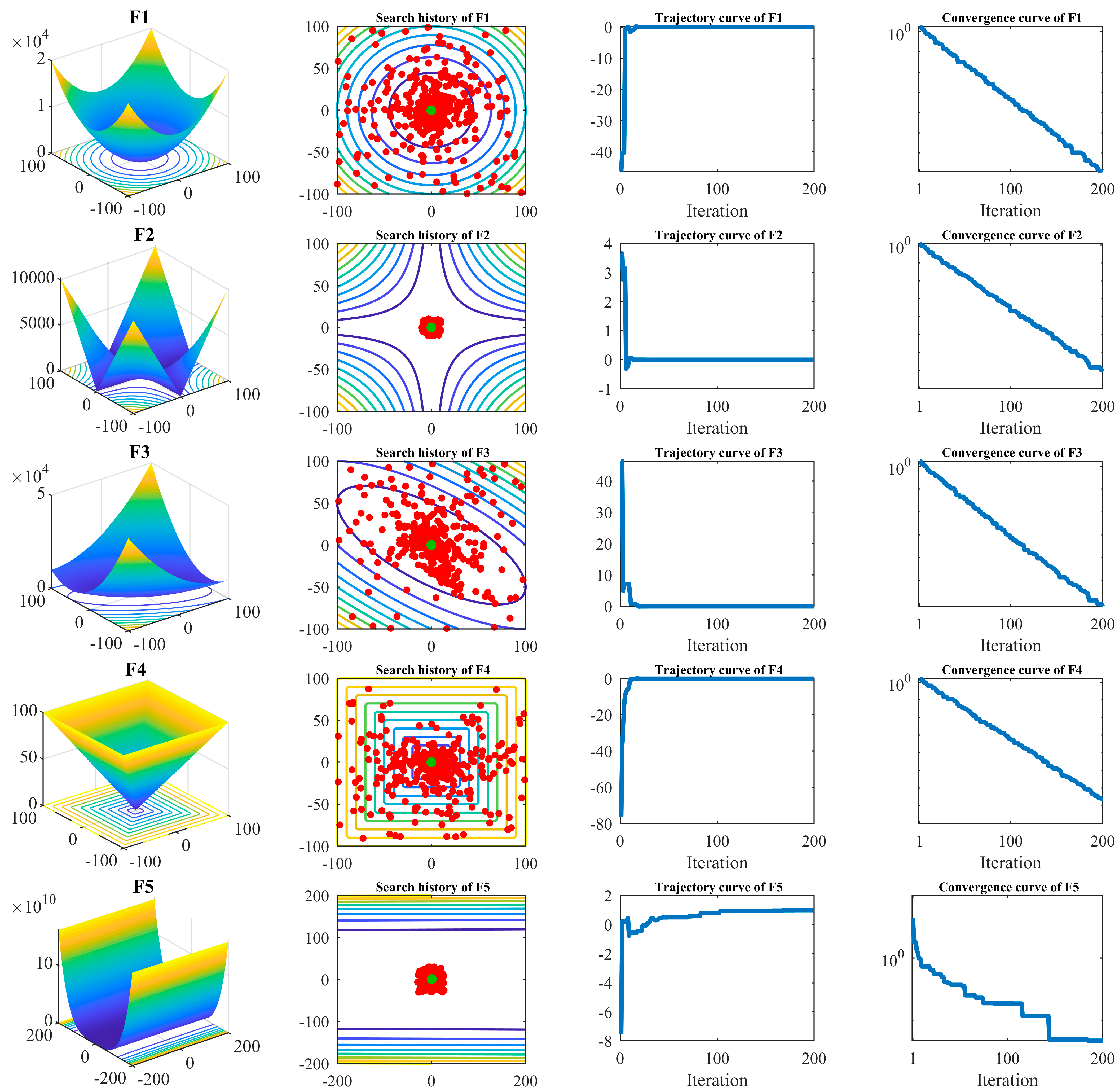
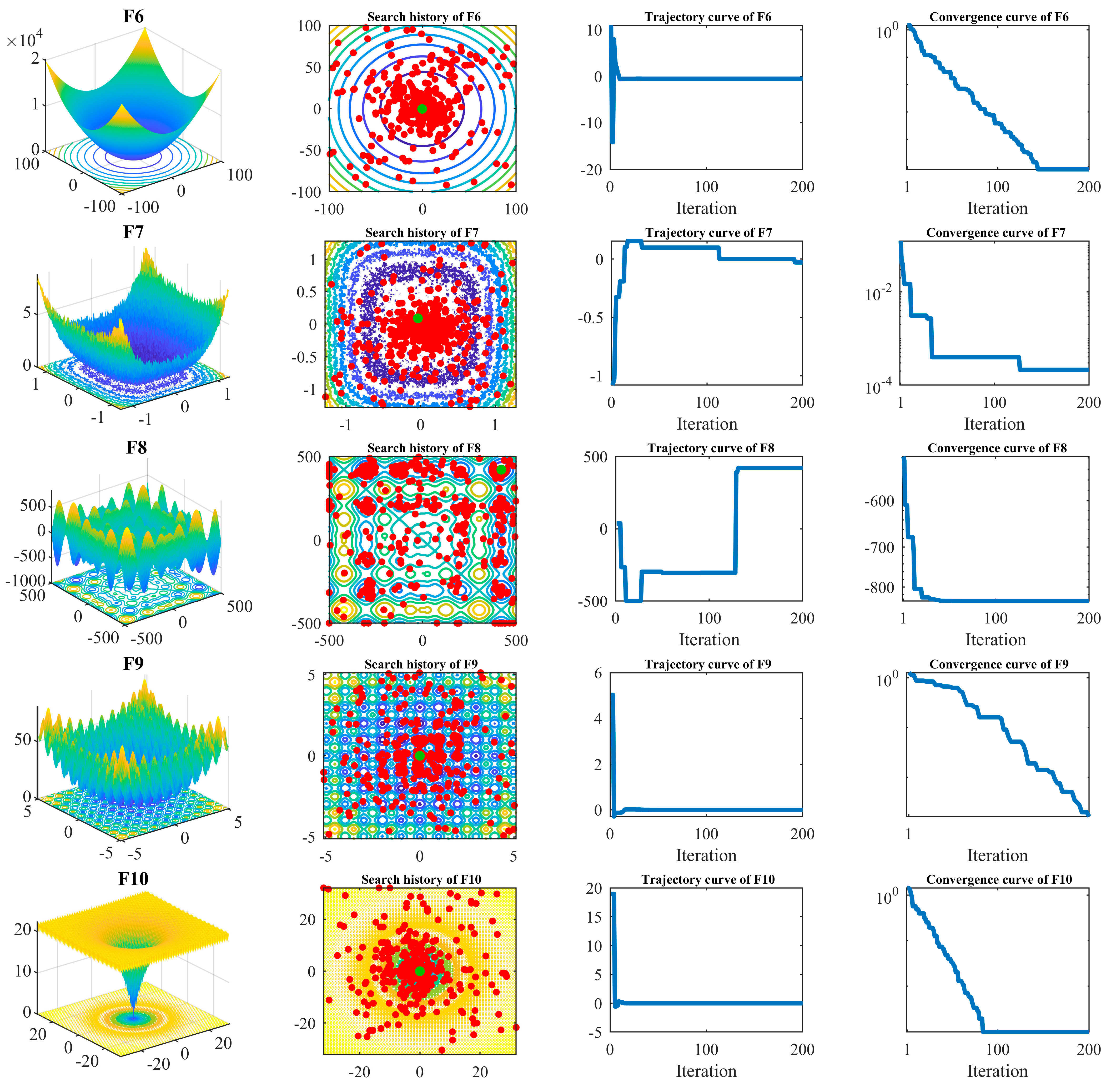
4.1. Intuitive Analysis in Two-Dimensional Search Space

Next, to visually observe the optimization process of the OOBO approach, the OOBO function was implemented in ten objective functions, F 1 to F 10 , in two dimensions. In this experiment, the number of OOBO population members was considered equal to five. To show the mechanism of the OOBO algorithm in solving the problems related to F 1 to F 10 , convergence curves, search history curves, and trajectory curves are presented in Figure 1. The horizontal axis in convergence curves and trajectory curves represents the number of iterations of the algorithm. These curves display OOBO’s behavior in scanning the problem-search space, solution-finding, the convergence process, and how it achieves better solutions based on update processes after each iteration, as well as decreasing the objective function values. What was concluded from the analysis of this experiment is that the OOBO approach, by improving the initial candidate solutions during the progress of the algorithm iterations, can converge towards the optimal solution, providing acceptable quasi-optimal solutions for the given problem.

4.2. Experimental Setup

To further analyze the quality of OOBO, the results obtained from this algorithm were compared with eight well-known optimization algorithms: PSO, TLO, GWO, WOA, MPA, TSA, GSA, and GA. The reasons for choosing these competitor algorithms were as follows: GA and PSO are among the most famous and widely used optimization algorithms that have been employed in many applications; GSA, TLBO, and GWO are highly cited algorithms, which shows that they have always been trusted and used by researchers. Additionally, WOA, MPA, and TSA are methods that have been published recently, and because of their acceptable performance, they have been favored by many researchers in this short period of publication. Therefore, in total, eight competitor algorithms in this study were selected, based on the following three criteria:
(i)
The most widely used algorithms: GA and PSO.
(ii)
Highly cited algorithms: GSA, TLBO, and GWO.
(iii)
Recently published and widely used algorithms: WOA, MPA, and TSA.
The values used for the control parameters of these competitors are specified in Table 1. To provide a fair comparison, standard versions of metaheuristic algorithms are used. Experiments were implemented on the software MATLAB R2022a utilizing a 64-bit Core i7 processor with 3.20 GHz and 16 GB main memory.

4.3. Performance Comparison

The ability of OOBO was compared with eight competitor algorithms applied to different objective functions of unimodal and multimodal types. Five indicators (mean, best, worst, standard deviation, and median) of the best-found solutions were used to report the performance results of the algorithms. To optimize each of the objective functions, OOBO was implemented in 20 independent runs, each of which contained 1000 iterations. Convergence curves for each benchmark function were drawn based on the average performance of metaheuristic algorithms in 20 independent runs. Random optimization algorithms are stochastic-based approaches that can provide a solution to the problem in an iterative process. An essential point in implementing optimization algorithms is determining the stopping rule for the algorithm iterations. There are various stopping rules (criteria) for optimization algorithms, including the total number of iterations, the total number of function evaluations, no change in the value of the objective function after a certain number of iterations, and determining an error level between the values of the objective function in several consecutive repetitions. Among them, the total number of iterations has been the focus of researchers, who employ this criterion for the stopping rule. Hence, the present investigation considered the total number of iterations (T) as a stopping rule for optimization algorithms in solving the functions F1 to F23 and function evaluations (FEs) in solving the CEC 2017 test suite.
Seven unimodal structures were included in the first group of objective functions analyzed to assess the competence of OOBO. Table 2 reports the implementation results of OOBO and eight competitors. What is clear from the analysis of the simulation results is that OOBO is the first best optimizer for the functions F 1 , F 2 , F 3 , F 4 , F 5 , F 6 , and F 7 compared to the competitor algorithms. The comparison of the simulation results demonstrates that the proposed OOBO has a great capacity to solve unimodal problems and is far more competitive than the other eight algorithms.
The second set of objective functions chosen to assess the efficacy of optimization algorithms consisted of six high-dimensional multimodal objective functions, F 8 to F 13 . Table 3 presents the outcomes of optimizing these objective functions utilizing the proposed OOBO and eight competitor techniques. Based on the simulation results, OOBO provides the optimal solution for F 9 and F 11 and is also the first-best optimizer for F 8 , F 10 , F 12 , and F 13 . Similarly, it was determined that OOBO has a more efficient ability to provide suitable solutions for F 8 to F 13 in relation to the competitor algorithms.
Ten fixed-dimensional multimodal functions were considered as the third group of objective functions to test the performance of the optimization techniques. Table 4 provides the outcomes of implementing the proposed OOBO and eight competitor algorithms on F 14 to F 23 . The simulation results reveal that OOBO outperforms the competitor algorithms for F 14 , F 15 , F 20 , F 21 , F 22 , and F 23 . In optimizing the functions F 16 , F 17 , F 18 , and F 19 , although from the “mean” perspective, the performance of several algorithms is the same, OOBO has better “standard deviation,” providing adequate solutions. The simulation results demonstrate that OOBO is more efficient than the competitor algorithms at solving this sort of objective functions.
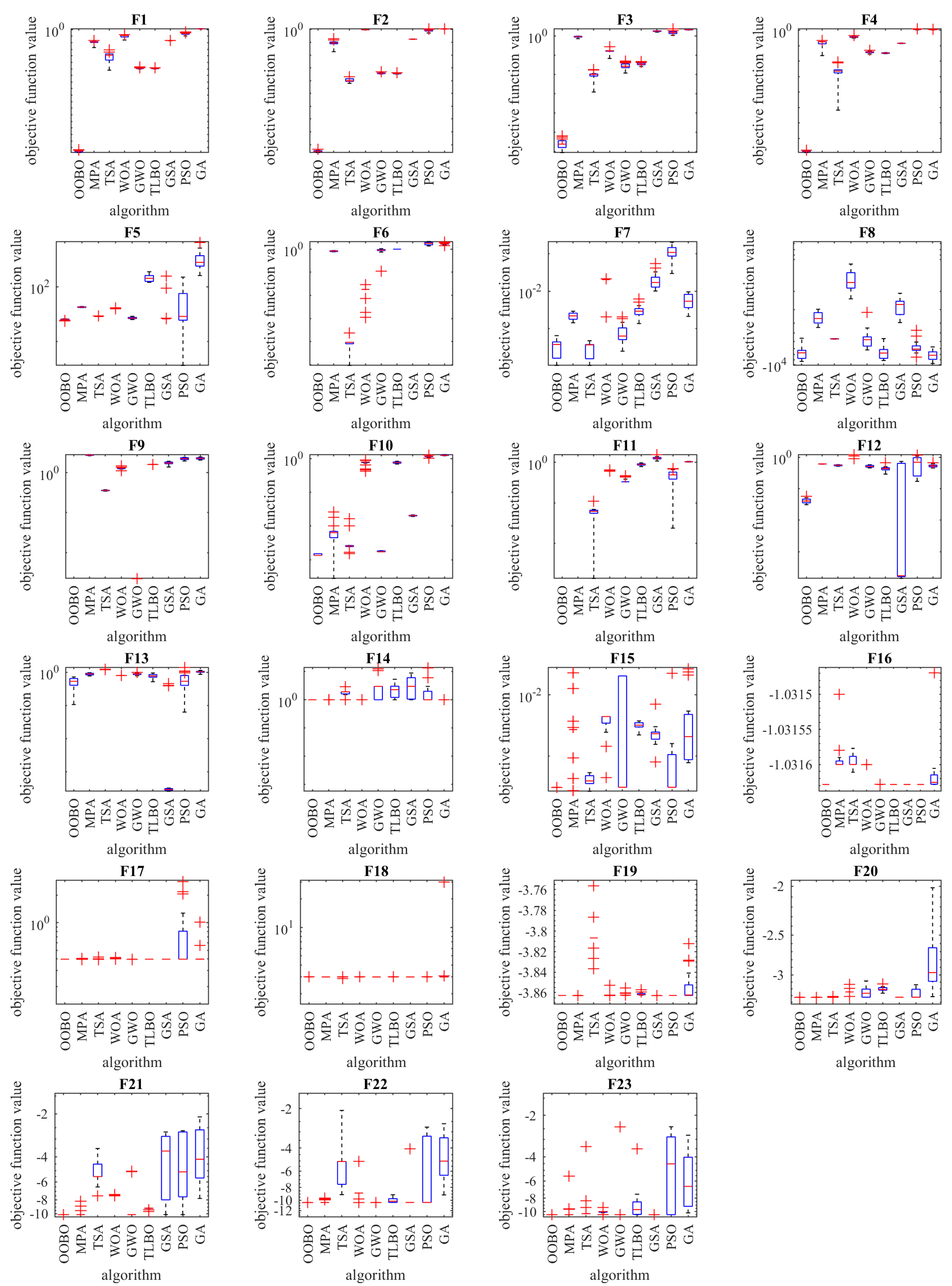
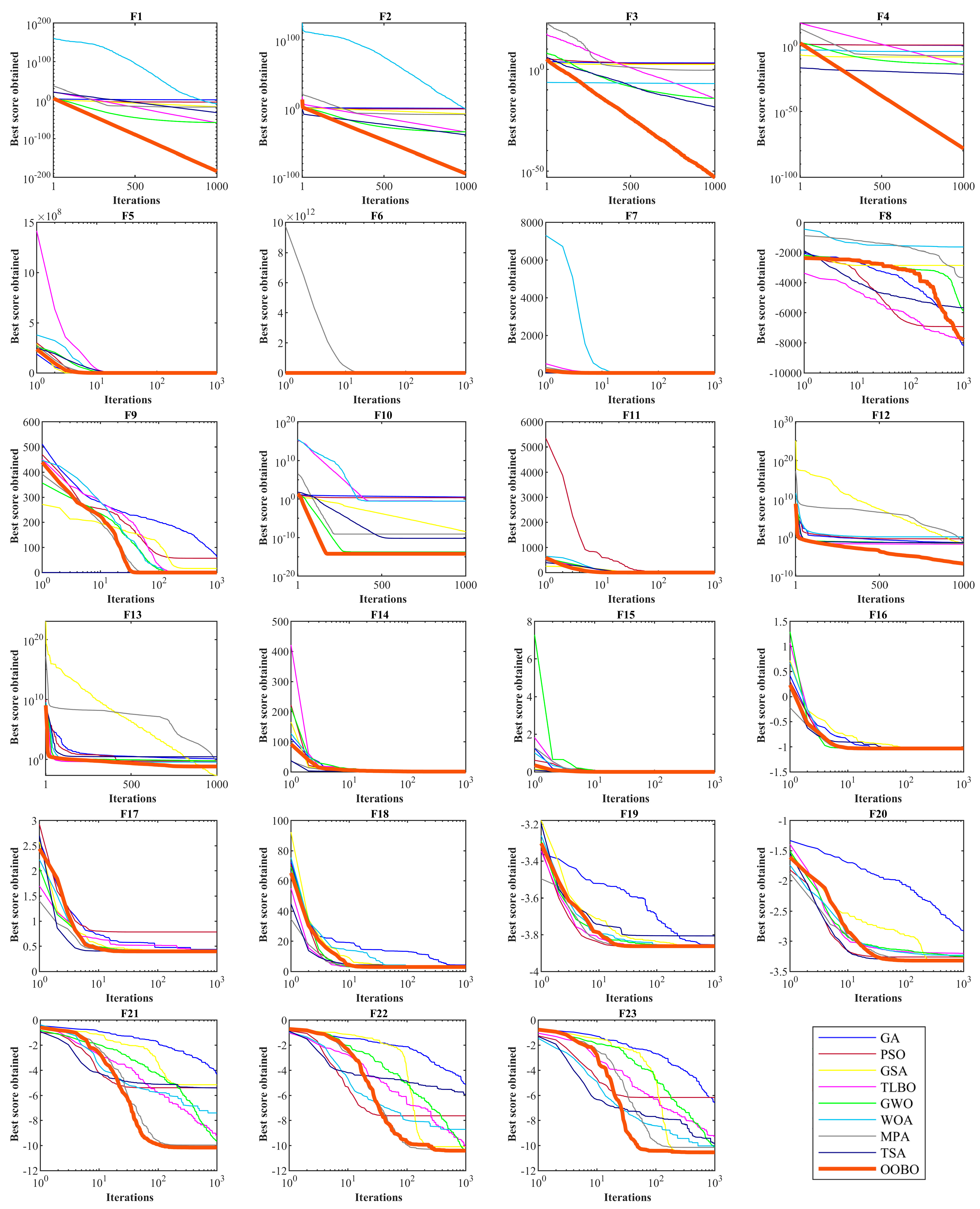
Figure 2 depicts a boxplot of the performance of optimization algorithms in solving objective functions F 1 to F 23 . In addition, the convergence curves of the OOBO approach and all competitor algorithms for benchmark functions F 1 to F 23 are presented in Figure 3. The best score in convergence curves refers to the best value obtained for the objective function up to each iteration. This index is updated in each iteration based on the comparison with its value in the previous iteration. The analysis of the convergence curves indicates that, when solving unimodal problems with objectives functions F 1 to F 7 , the proposed OOBO converges on much better solutions than its eight competitor algorithms, and it has superior performance. When solving high-dimensional multi-model problems based on F 8 to F 13 , OOBO has a greater convergence strength than its eight competitor algorithms. When solving high-dimensional multi-model problems using F 14 to F 23 , the proposed OOBO approach has a faster convergence speed and greater convergence strength than eight competitor algorithms.

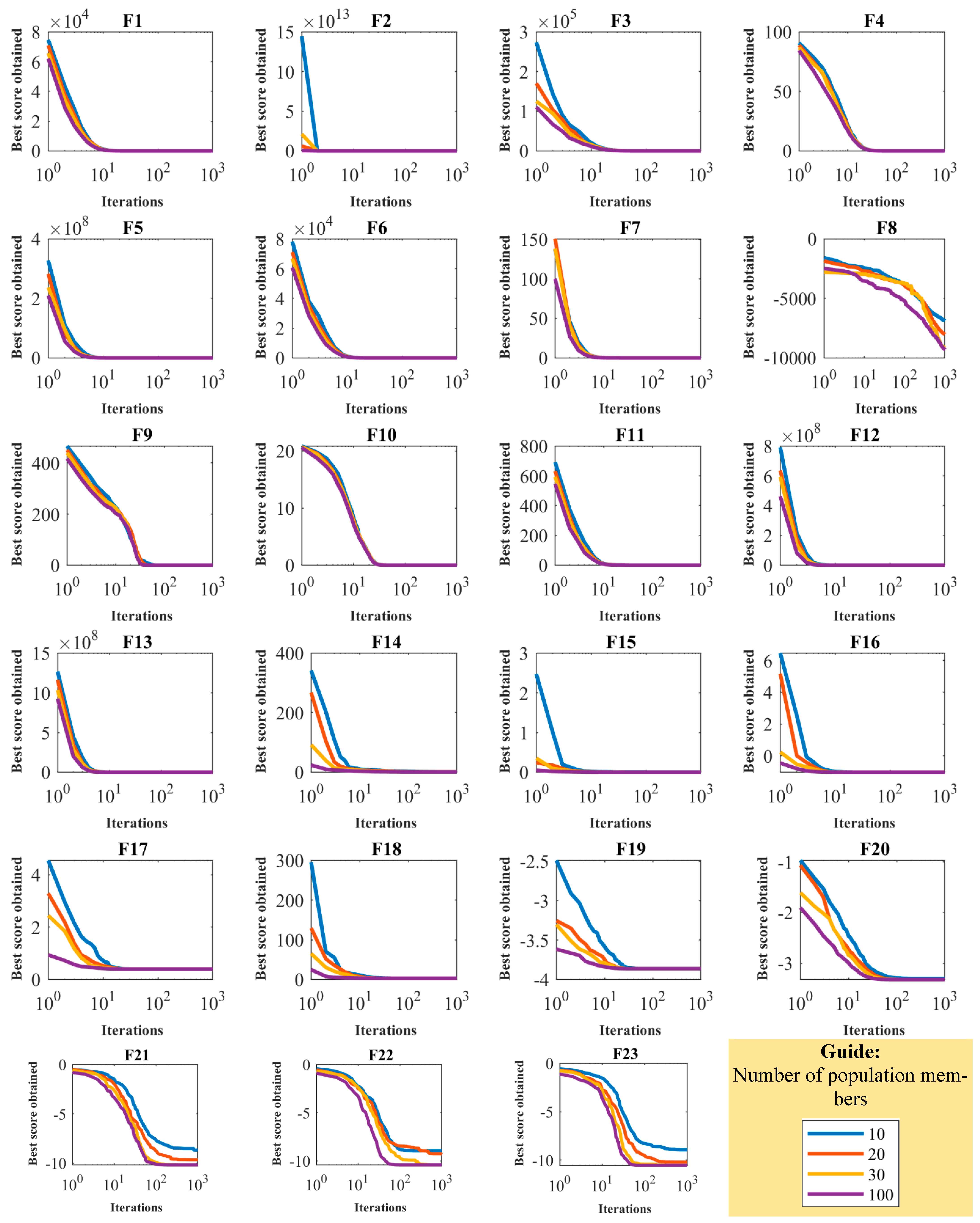
4.4. Sensitivity Analysis

The proposed OOBO employs two parameters, the number of population members ( N ) and the maximum number of iterations ( T ) in the implementation process, to solve optimization problems. In this regard, the analysis of OOBO’s sensitivity to these two parameters was assessed next. OOBO was implemented in independent runs for different values of N = 10, 20, 30, and 100 on F 1 to F 23 to investigate the sensitivity of the proposed method to the number of population members’ parameter. The simulation results of this part of the study are reported in Table 5, whereas the behavior of the convergence curves under the impact of changes in population size is displayed in 
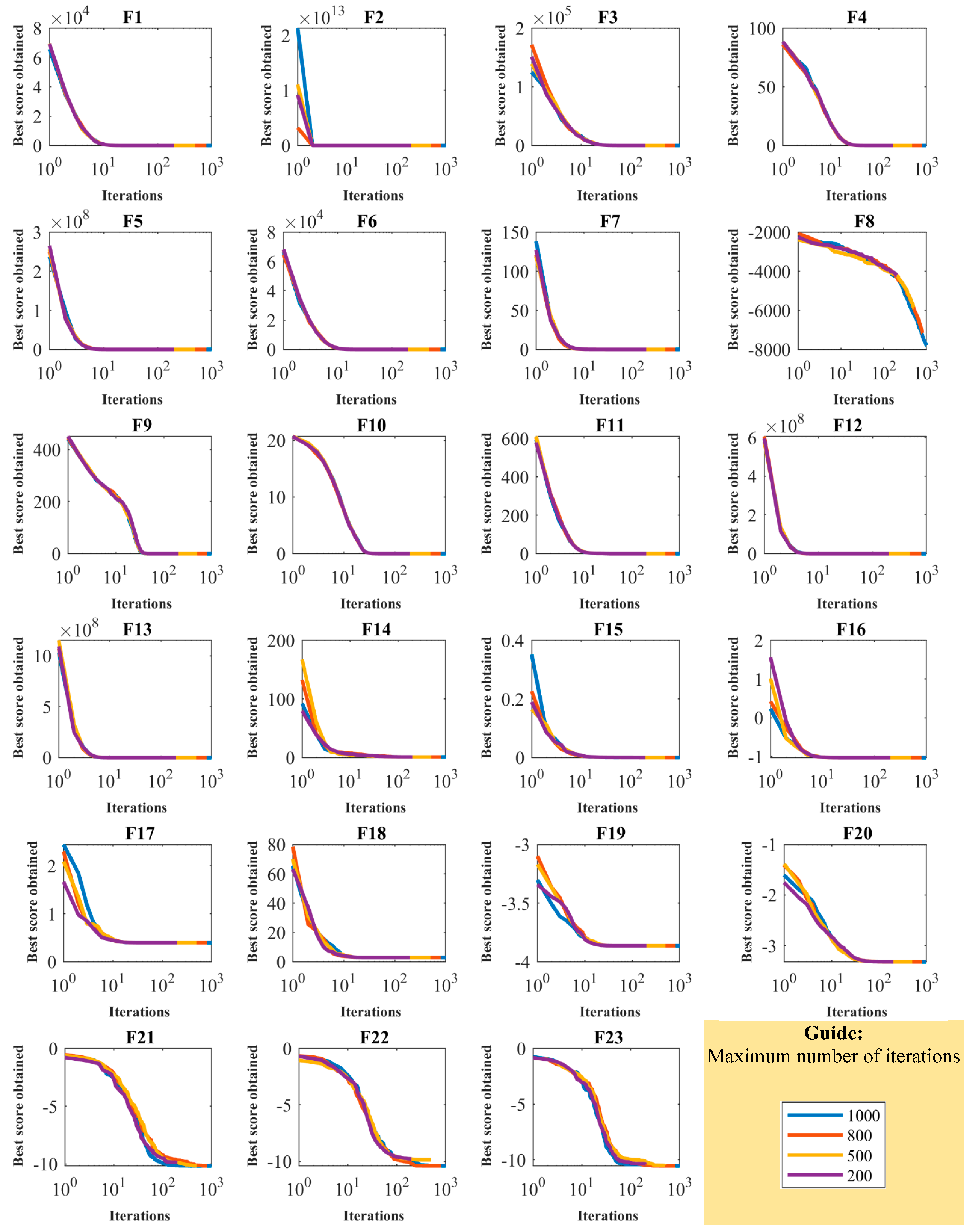
Figure 4. The simulation results show that the values of all objective functions decline as the population size increases. To investigate the proposed algorithm’s sensitivity in relation to T , OOBO is employed in independent runs with different values of this parameter equal to T = 200, 500, 800, and 1000 for optimizing the functions F 1 to F 23 . Table 6 and Figure 5 show the results of the sensitivity analysis of OOBO regarding T . The inference from the OOBO sensitivity analysis with the parameter T is that this algorithm can converge on better optimal solutions when employed in a larger number of iterations.

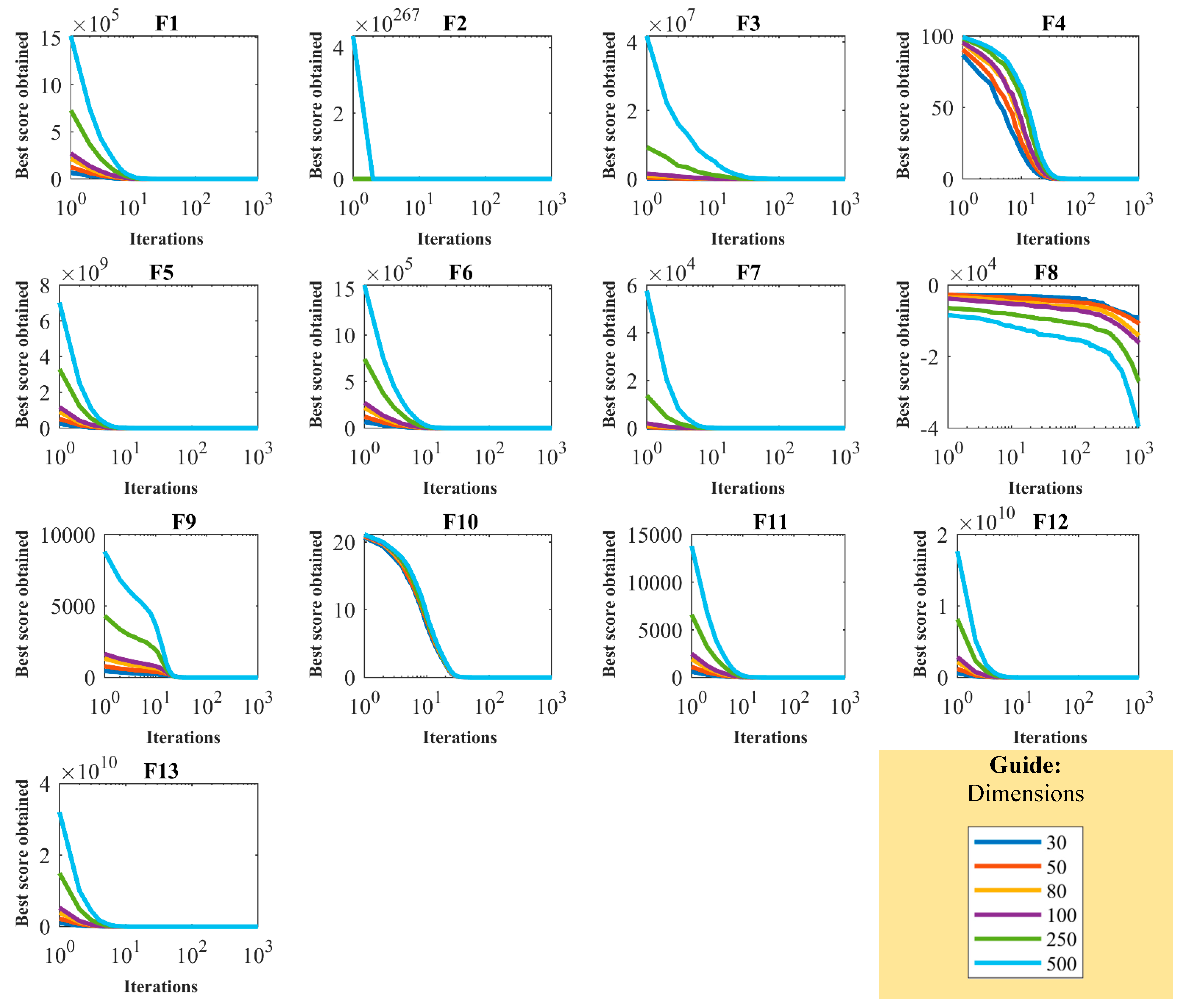
4.5. Scalability Analysis

Next, a scalability study is presented to analyze the performance of OOBO in optimizing objective functions under the influence of changes in the problem dimensions. For this purpose, OOBO was employed in different dimensions (30, 50, 80, 100, 250, and 500) in optimizing F 1 to F 13 . The OOBO convergence curves in solving objective functions for the various mentioned dimensions are presented in Figure 6. The simulation results obtained from the scalability study are reported in Table 7. From the analysis of the results in this table, we can deduce that the efficiency of OOBO is not degraded too much when the dimensions of the given problem increase. OOBO’s optimal performance under the influence of changes in the problem dimensions is due to OOBO’s ability to achieve the proper balance between exploration and exploitation.

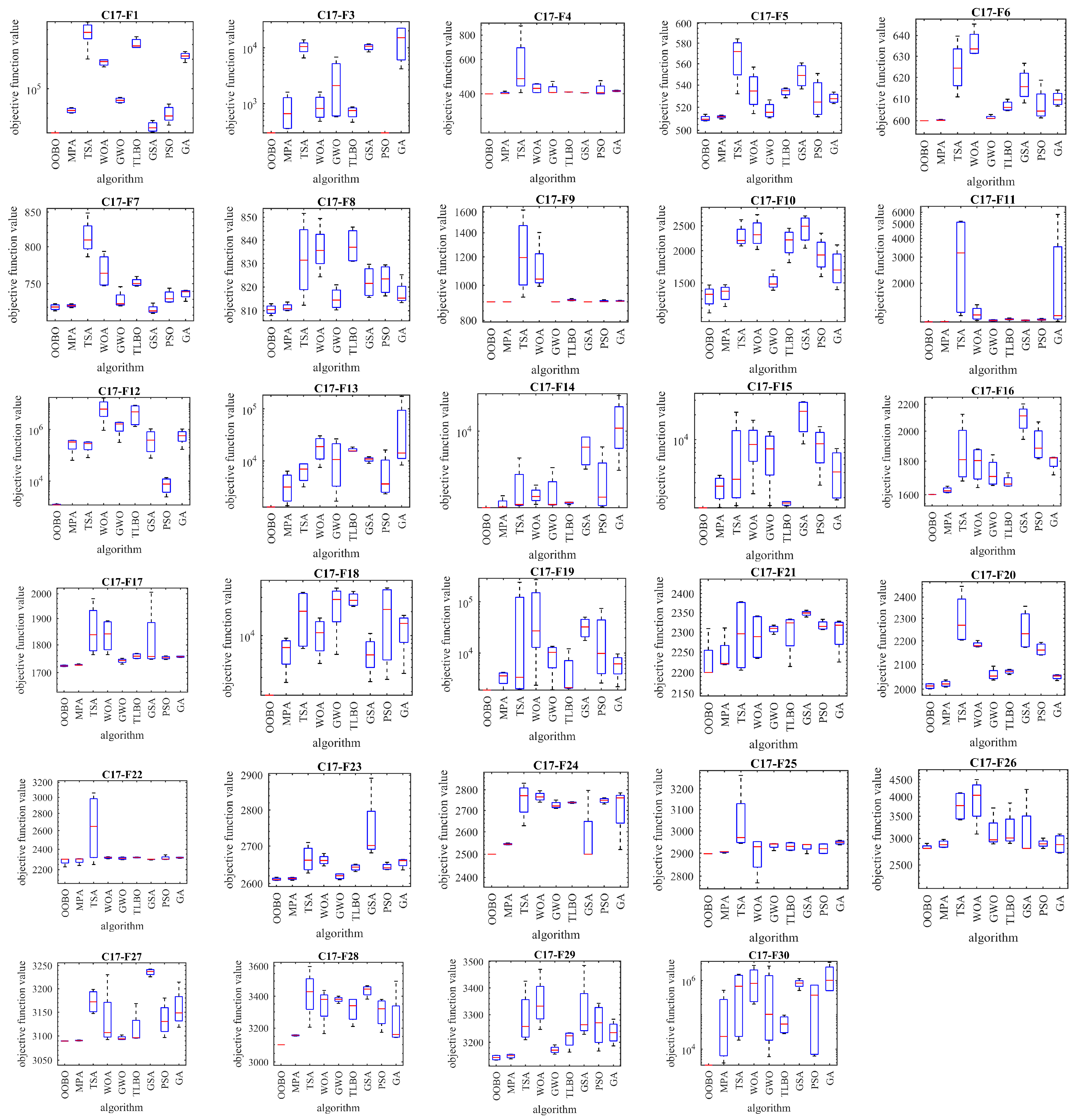
4.6. Evaluation of the CEC 2017 Test Suite

Next, the performance of the proposed OOBO approach in handling the CEC 2017 test suite was evaluated. The CEC 2017 test suite has thirty benchmark functions consisting of three unimodal functions, C17-F1 to C17-F3, seven multimodal functions, C17-F4 to C17-F10, ten hybrid functions, C17-F11 to C17-F20, and ten composition functions, C17-F21 to C17-F30. The function C17-F2 was removed from this test suite due to unstable behavior (as in similar papers). The unstable behavior of C17-F2 means that, especially for higher dimensions, it shows significant performance variations for the same algorithm implemented in Matlab. Complete information on the CEC 2017 test suite is provided in [77]. The implementation results of OOBO and competitor algorithms with the CEC 2017 test suite are reported in Table 8. The boxplot diagrams obtained from the performance of the metaheuristic algorithms in handling the CEC 2017 test suite are drawn in Figure 7.
Based on the simulation results, OOBO is the first-best optimizer for the functions C17-F1, C17-F4 to C17-F6, C17-F8, C17-F10 to C17-24, and C17-F26 to C17-F30. The analysis of the simulation results shows that the proposed OOBO approach has been able to provide superior performance in solving the CEC 2017 test suite by providing better results in most of the benchmark functions compared to competitor algorithms.

4.7. Statistical Analysis

Next, the Wilcoxon rank sum test [78] was utilized to evaluate the performance of optimization algorithms in addition to statistical analysis of the average and standard deviation. The Wilcoxon rank sum test is used to determine whether there is a statistically significant difference between two sets of data. A p-value in this test reveals whether the difference between OOBO and each of the competitor algorithms is statistically significant. Table 9 reports the results of our statistical analysis. Based on the analysis of the simulation results, the proposed OOBO has a p-value less than 0.05 in each of the three types of objective functions compared to each of the competitor algorithms. This result indicates that OOBO is significantly different in statistical terms from the eight compared algorithms.

5. OOBO for Real-World Applications

In this section, the proposed OOBO and eight competitor algorithms are applied to four science/engineering designs to evaluate their capacity to resolve real-world problems. These design problems are pressure vessel, speed reducer, welded beam, and tension/compression spring.

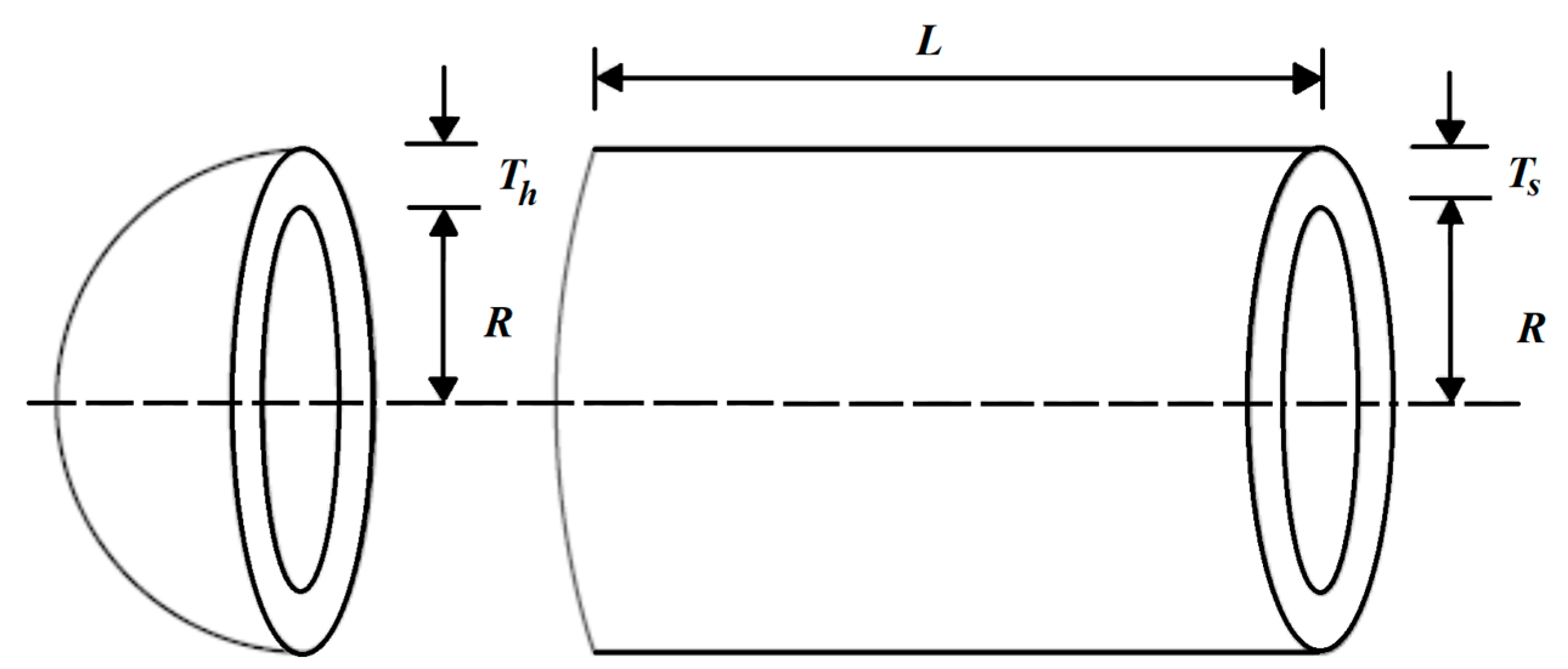
5.1. Pressure Vessel Design Problem

The mathematical model of the pressure vessel design problem was adapted from [79]. The main goal of this problem is to minimize the design cost. A schematic view of the pressure vessel design problem is shown in Figure 8.
To formulate the model, consider that X = x 1 ,   x 2 ,   x 3 ,   x 4 = T s ,   T h ,   R ,   L , and then the mathematical program is given by
Minimize:
f x = 0.6224 x 1 x 3 x 4 + 1.778 x 2 x 3 2 + 3.1661 x 1 2 x 4 + 19.84 x 1 2 x 3
Subject to:
g 1 x = x 1 + 0.0193 x 3     0 ,  
g 2 x = x 2 + 0.00954 x 3   0 ,
g 3 x = π x 3 2 x 4 4 3 π x 3 3 + 1296000   0 ,  
g 4 x = x 4 240     0 ,
with 0 x 1 ,   x 2 100   a n d   10 x 3 ,   x 4 200 .
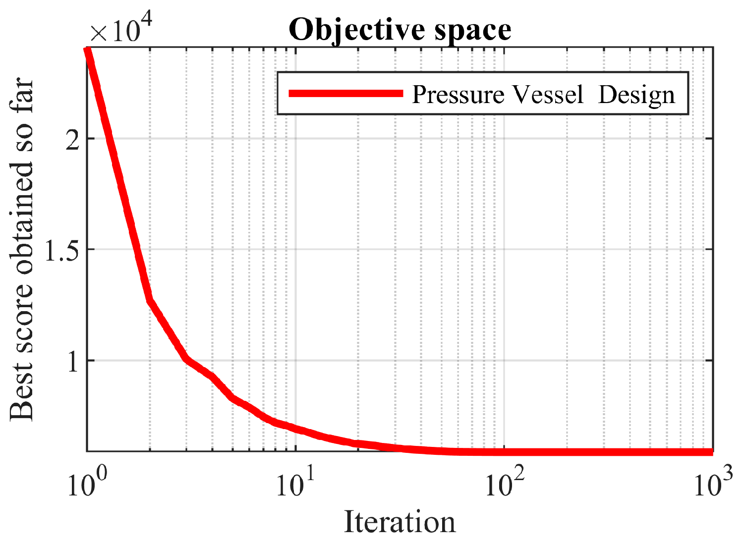
The obtained solutions using OOBO and eight competitor algorithms are presented in Table 10. Based on the results of this table, OOBO presented the optimal solution at (0.7781, 0.3832, 40.3150, 200), and the value of the objective function was equal to 5870.8460. An analysis of the results of this table showed that the proposed OOBO has good performance in solving the problem at a low cost. The statistical results of the performance of the optimization algorithms when solving this problem are presented in Table 11. These results indicated that OOBO provides better values for the best, mean, and median indices than the other eight compared algorithms. The convergence curve of the proposed OOBO is presented in Figure 9 while achieving the optimal solution.

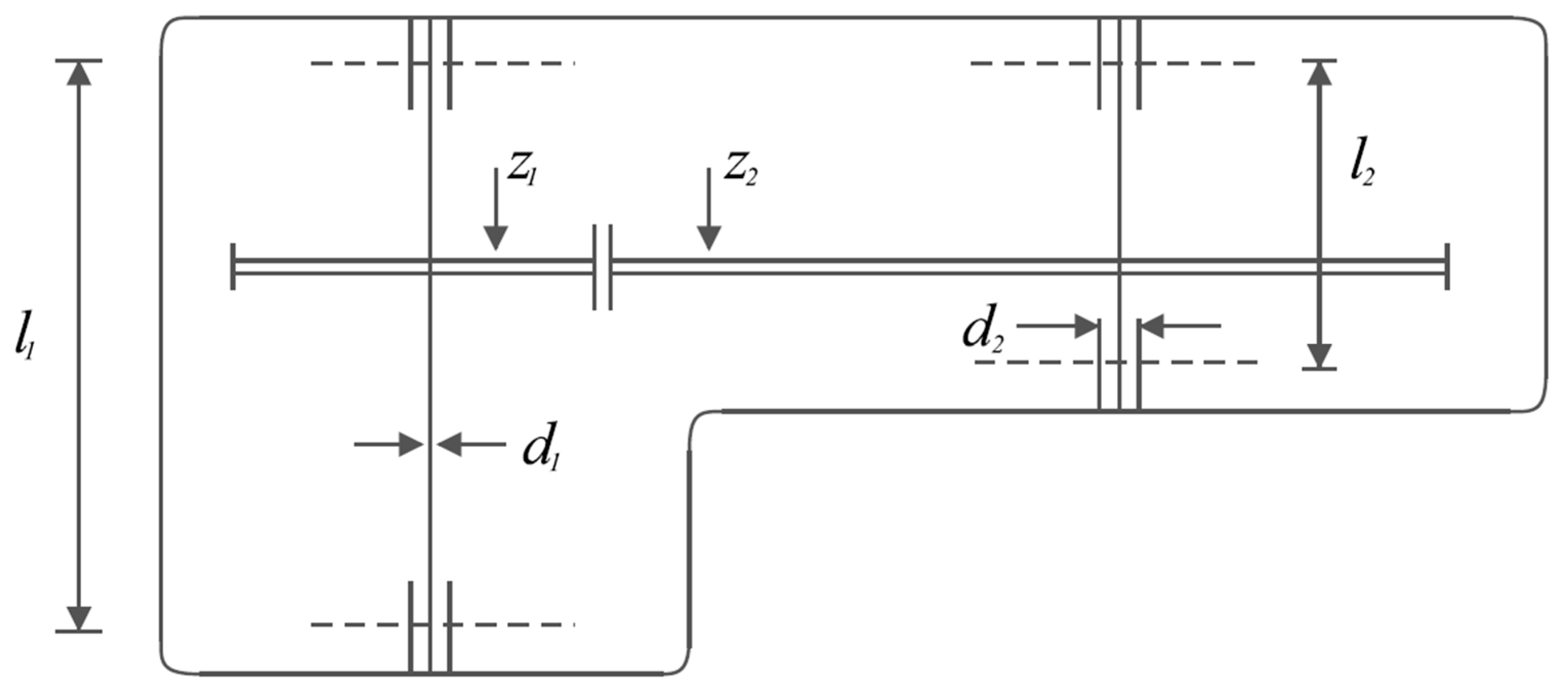
5.2. Speed Reducer Design Problem

The mathematical model of the speed reducer design problem was first formulated in [80], but we used an adapted formulation from [81]. The main goal of this problem is to minimize the weight of the speed reducer. A schematic view of the speed reducer design problem is shown in Figure 10.
To formulate the model, consider that X = x 1 , x 2 , x 3 , x 4 , x 5 , x 6 , x 7 = b , m , p , l 1 , l 2 , d 1 , d 2 , and then the mathematical program is given by
Minimize:
f x = 0.7854 x 1 x 2 2 3.3333 x 3 2 + 14.9334 x 3 43.0934 1.508 x 1 x 6 2 + x 7 2 + 7.4777 x 6 3 + x 7 3 + 0.7854 ( x 4 x 6 2 + x 5 x 7 2 )
Subject to:
g 1 x = 27 x 1 x 2 2 x 3 1     0 ,   g 2 x = 397.5 x 1 x 2 2 x 3 1   0 ,
g 3 x = 1.93 x 4 3 x 2 x 3 x 6 4 1   0 ,   g 4 x = 1.93 x 5 3 x 2 x 3 x 7 4 1     0 ,
g 5 x = 1 110 x 6 3 745 x 4 x 2 x 3 2 + 16.9 · 10 6 1   0 ,
g 6 ( x ) = 1 85 x 7 3 745 x 5 x 2 x 3 2 + 157.5 · 10 6 1     0 ,
g 7 x = x 2 x 3 40 1     0 ,   g 8 x = 5 x 2 x 1 1     0 ,
g 9 x = x 1 12 x 2 1     0 ,  
g 10 x = 1.5 x 6 + 1.9 x 4 1     0 ,
  g 11 x = 1.1 x 7 + 1.9 x 5 1     0 ,
with
2.6 x 1 3.6 ,   0.7 x 2 0.8 ,   17 x 3 28 ,   7.3 x 4 8.3 ,   7.8 x 5 8.3 ,   2.9 x 6 3.9
and
5 x 7 5.5 .
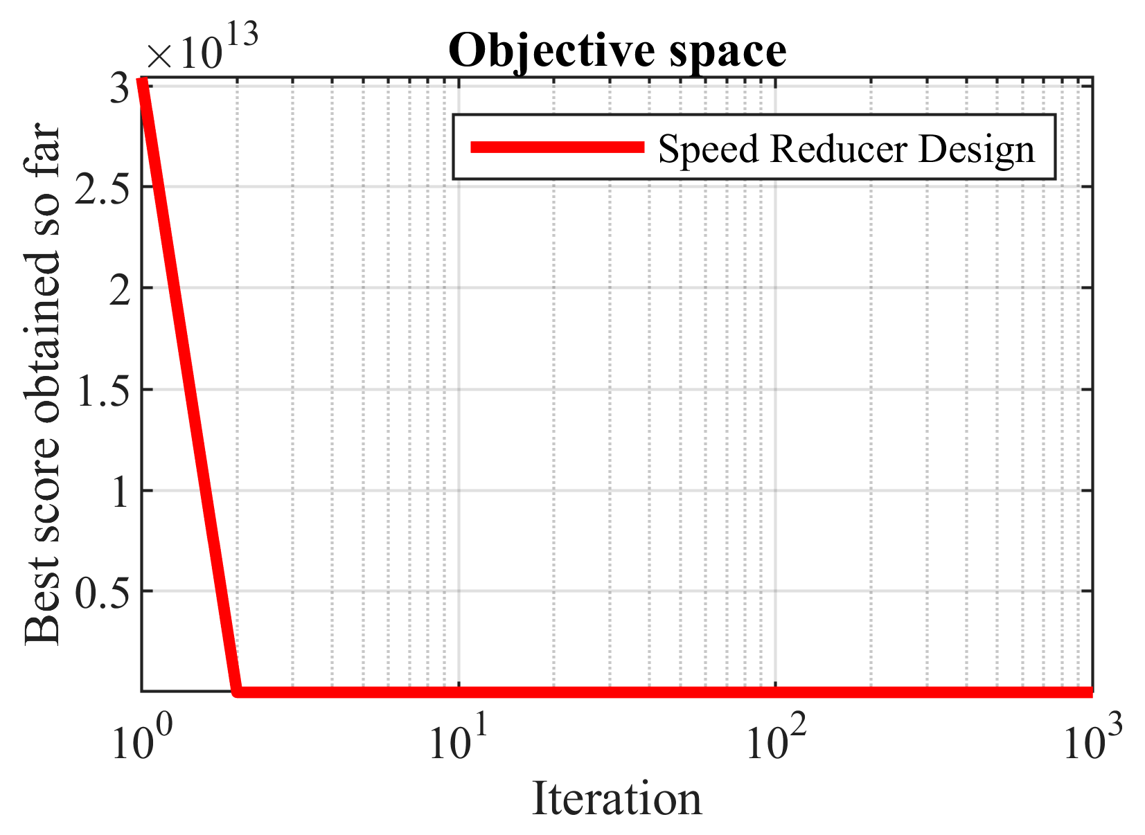
The results of the implementation of the proposed OOBO and eight compared algorithms on this problem are presented in Table 12. OOBO presented the optimal solution at (3.5012, 0.7, 17, 7.3, 7.8, 3.33412, 5.26531) with an objective function value of 2989.8520. Table 13 presents the statistical results obtained from the proposed OOBO and eight competitor algorithms. Based on the simulation results, OOBO has superior performance over the eight algorithms when solving the speed reducer design problem. The convergence curve of the proposed OOBO is presented in Figure 11.

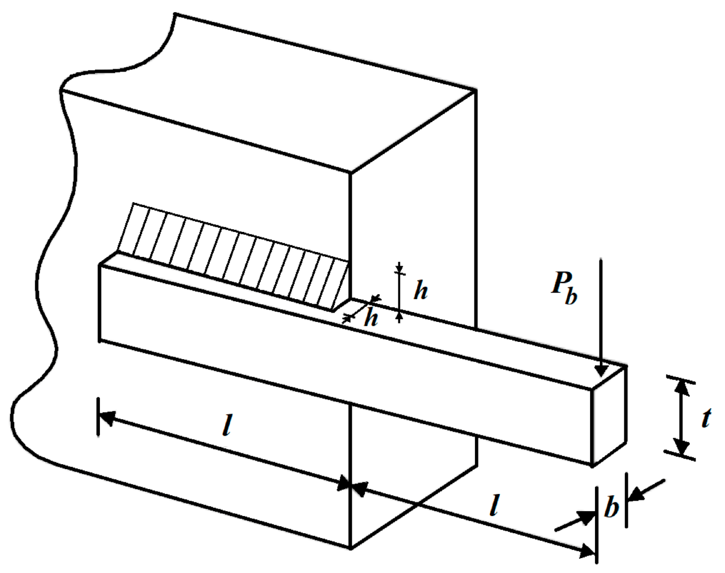
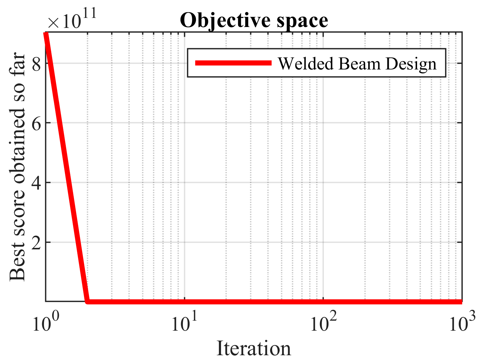
5.3. Welded Beam Design

The mathematical model of a welded beam design was adapted from [22]. The main goal for solving this design problem is to minimize the fabrication cost of the welded beam. A schematic view of the welded beam design problem is shown in Figure 12.
To formulate the model, consider that X = x 1 ,   x 2 ,   x 3 ,   x 4 = h ,   l ,   t ,   b , and then the mathematical program is given by
Minimize:
f ( x ) = 1.10471 x 1 2 x 2 + 0.04811 x 3 x 4   ( 14.0 + x 2 )
Subject to:
g 1 x = τ x 13600     0 ,  
g 2 x = σ x 30000     0 ,
g 3 x = x 1 x 4   0 ,  
g 4 ( x ) = 0.10471 x 1 2 + 0.04811 x 3 x 4   ( 14 + x 2 ) 5.0     0 ,
g 5 x = 0.125 x 1   0 ,  
g 6 x = δ   x 0.25     0 ,
g 7 x = 6000 p c   x   0 ,
where
τ x = τ 2 + 2 τ τ x 2 2 R + τ 2   ,   τ = 6000 2 x 1 x 2 ,   τ = M R J ,
M = 6000 14 + x 2 2 ,   R = x 2 2 4 + x 1 + x 3 2 2 ,
J = 2 2 x 1 x 2 x 2 2 12 + x 1 + x 3 2 2   ,   σ x = 504000 x 4 x 3 2   , δ   x = 65856000 30 · 1 0 6 x 4 x 3 3   ,
  p c   x = 4.013 30 · 1 0 6 x 3 x 4 3 1176 1 x 3 28 30 · 1 0 6 4 ( 12 · 1 0 6 )   ,
with 0.1 x 1 , x 4 2 a n d 0.1 x 2 , x 3 10 .
The results of the implementation of the proposed OOBO and the compared algorithms on this problem are presented in Table 14. The simulation results show that the proposed algorithm presented the optimal solution at (0.20328, 3.47115, 9.03500, 0.20116) with an objective function value of 1.72099. An analysis of the statistical results of the implemented algorithms is presented in Table 15. Based on this analysis, note that the proposed OOBO is superior to the compared algorithms in providing the best, mean, and median indices. The convergence curve of OOBO to solve the welded beam design problem is shown in Figure 13.

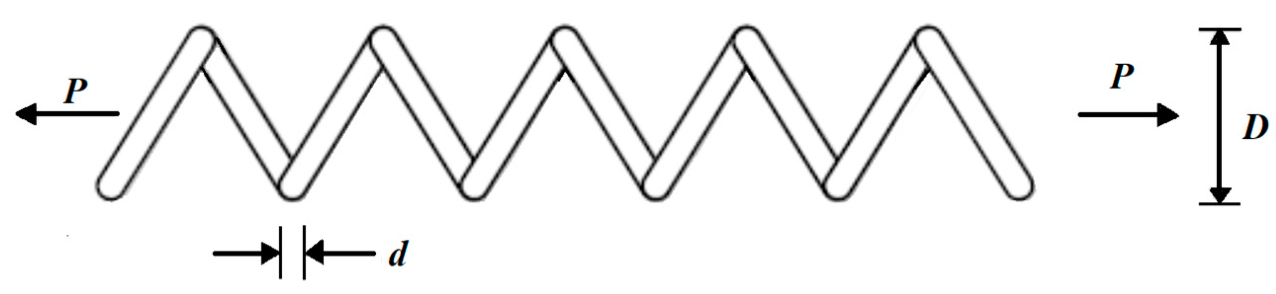
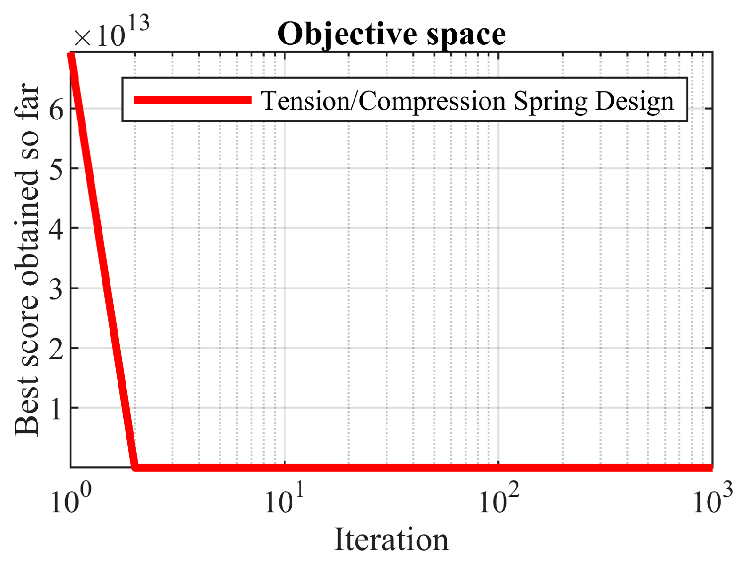
5.4. Tension/Compression Spring Design

The mathematical model of this problem was adapted from [22]. The main goal of this design problem is to minimize the tension/compression of the spring weight. A schematic view of the tension/compression spring design problem is shown in Figure 14.
To formulate the model, consider that X = x 1 ,   x 2 ,   x 3   = d ,   D ,   P , and then the mathematical program is given by
Minimize:
f x = x 3 + 2 x 2 x 1 2
Subject to:
g 1 x = 1 x 2 3 x 3 71785 x 1 4     0 ,  
g 2 x = 4 x 2 2 x 1 x 2 12566 ( x 2 x 1 3 x 1 4 ) + 1 5108 x 1 2 1   0 ,
g 3 x = 1 140.45 x 1 x 2 2 x 3   0 ,   g 4 x = x 1 + x 2 1.5 1     0 ,
with 0.05 x 1 2 , 0.25 x 2 1.3 a n d 2 x 3 15 .
The performance of all optimization algorithms in achieving the objective values and design variables values is presented in Table 16. The optimization results show that the proposed OOBO provided the optimal solution at (0.05107, 0.34288, 12.08809) with an objective function value of 0.01266. A comparison of the results showed that OOBO has superior performance in solving this problem compared to those of the other eight algorithms. A comparison of the statistical results of the performance of the proposed OOBO against the eight competitor algorithms is provided in Table 17. The analysis of this table reveals that OOBO offers a more competitive performance in providing the best, mean, and median indices. The convergence curve of the proposed OOBO in achieving the obtained optimal solution is shown in Figure 15.

6. Conclusions and Future Works

A new optimization technique called one-to-one-based optimizer (OOBO) was proposed in this study. The main idea in designing OOBO was the participation of all population members in the algorithm’s updating process based on a one-to-one correspondence between the two sets of members of the population and a set of selected members as guides. Thus, each population member was selected precisely once as a guide to another member and then used to update the position of that population member. The performance of the proposed OOBO in solving optimization problems was tested on 52 objective functions belonging to unimodal, high-dimensional, and fixed-dimensional multimodal types, as well as the CEC 2017 test suite. The findings indicated OOBO’s strong ability in exploitation based on the results of unimodal functions, OOBO’s strong ability in exploration based on the results of high-dimensional multimodal functions, and OOBO’s acceptability in balancing exploitation and exploration based on the results of fixed-dimensional multimodal, hybrid, and composition functions.
In addition, the performance of the proposed approach in solving optimization problems was compared with eight well-known algorithms. Simulation results reported that the proposed algorithm provided quasi-optimal solutions with better convergence than the compared algorithms. Furthermore, the power of the proposed approach to provide suitable solutions for real-world applications was tested by applying it to four science/engineering design problems. It is clear from the optimization results of this experiment that the proposed OOBO is applicable to solving real-world optimization problems. In response to the main research question about introducing a new optimization algorithm, the simulation findings showed that the proposed OOBO approach performed better in most of the benchmark functions than its competing algorithms. The successful and acceptable performance of OOBO justifies the introduction and design of the proposed approach.
Against advantages such as a strong ability to balance exploration and exploitation and effectiveness in handling real-world applications, the proposed OOBO approach has limitations and disadvantages. The first limitation for all optimization algorithms is that, based on the NFL theorem, there is always a possibility that newer algorithms will be designed that perform better than OOBO. A second limitation of OOBO is that there is no guarantee of achieving global optimization using it due to the nature of random search. Another limitation of OOBO is that, although it has provided successful performance in the optimization problems under study in this paper, there is no guarantee that it will provide similar performance in other optimization applications. Therefore, it is never and in no way claimed that OOBO is the best optimizer for all optimization applications.
The authors of this paper provide several study proposals for the present research. In this regard, we can mention the multi-objective version’s design and the binary version of the proposed OOBO algorithm. Moreover, the usage of OOBO for NP-hard/NP-complete problems, different applications, and optimization problems in science, engineering, data mining, data clustering, sensor placement, big data, medical, and feature selection is additional research potential for further studies based on this paper.

Author Contributions

Conceptualization, M.D., E.T. and O.P.M.; data curation, M.D., E.T. and P.T.; formal analysis, E.T., M.D. and O.P.M.; investigation, O.P.M. and E.T.; methodology, M.D., E.T. and P.T.; software, M.D. and E.T.; validation, M.D., E.T. and O.P.M.; visualization, E.T., M.D. and P.T.; writing—original draft preparation, M.D. and E.T.; writing—review and editing, P.T. and O.P.M. All authors have read and agreed to the published version of the manuscript.

Funding

“Professor O.P. Malik” (the fourth author) has paid APC from his NSERC, Canada, research grant.

Institutional Review Board Statement

Not applicable.

Informed Consent Statement

The authors declare no conflict of interest.

Data Availability Statement

Not applicable.

Acknowledgments

The authors thank the University of Hradec Králové for its support.

Conflicts of Interest

The authors declare no conflict of interest.

References

  1. Dhiman, G. SSC: A hybrid nature-inspired meta-heuristic optimization algorithm for engineering applications. Knowl.-Based Syst. 2021, 222, 106926. [Google Scholar] [CrossRef]
  2. Nocedal, J.; Wright, S. Numerical Optimization; Springer Science & Business Media: Berlin, Germany, 2006. [Google Scholar]
  3. Talbi, E.-G. Metaheuristics: From Design to Implementation; John Wiley & Sons: Hoboken, NJ, USA, 2009; Volume 74. [Google Scholar]
  4. Gu, Q.; Wang, Q.; Li, X.; Li, X. A surrogate-assisted multi-objective particle swarm optimization of expensive constrained combinatorial optimization problems. Knowl.-Based Syst. 2021, 223, 107049. [Google Scholar] [CrossRef]
  5. Iba, K. Reactive power optimization by genetic algorithm. IEEE Trans. Power Syst. 1994, 9, 685–692. [Google Scholar] [CrossRef]
  6. Dehghani, M.; Trojovský, P. Teamwork Optimization Algorithm: A New Optimization Approach for Function Minimization/Maximization. Sensors 2021, 21, 4567. [Google Scholar] [CrossRef]
  7. Wolpert, D.H.; Macready, W.G. No free lunch theorems for optimization. IEEE Trans. Evol. Comput. 1997, 1, 67–82. [Google Scholar] [CrossRef]
  8. Singh, P.; Dhiman, G.; Kaur, A. A quantum approach for time series data based on graph and Schrödinger equations methods. Mod. Phys. Lett. A 2018, 33, 1850208. [Google Scholar] [CrossRef]
  9. Kennedy, J.; Eberhart, R. Particle Swarm Optimization. In Proceedings of the ICNN’95—International Conference on Neural Networks, Perth, WA, Australia, 27 November–1 December 1995; Volume 4, pp. 1942–1948. [Google Scholar]
  10. Dorigo, M.; Maniezzo, V.; Colorni, A. Ant system: Optimization by a colony of cooperating agents. IEEE Trans. Syst. Man Cybern. Part B 1996, 26, 29–41. [Google Scholar] [CrossRef]
  11. Yang, X.S.; Gandomi, A.H. Bat algorithm: A novel approach for global engineering optimization. Eng. Comput. 2012, 29, 464–483. [Google Scholar] [CrossRef]
  12. Mirjalili, S.; Mirjalili, S.M.; Lewis, A. Grey wolf optimizer. Adv. Eng. Softw. 2014, 69, 46–61. [Google Scholar] [CrossRef]
  13. Dehghani, M.; Trojovský, P.; Malik, O.P. Green Anaconda Optimization: A New Bio-Inspired Metaheuristic Algorithm for Solving Optimization Problems. Biomimetics 2023, 8, 121. [Google Scholar] [CrossRef]
  14. Dhiman, G.; Kumar, V. Spotted hyena optimizer: A novel bio-inspired based metaheuristic technique for engineering applications. Adv. Eng. Softw. 2017, 114, 48–70. [Google Scholar] [CrossRef]
  15. Dehghani, M.; Hubálovský, Š.; Trojovský, P. Northern Goshawk Optimization: A New Swarm-Based Algorithm for Solving Optimization Problems. IEEE Access 2021, 9, 162059–162080. [Google Scholar] [CrossRef]
  16. Jiang, Y.; Wu, Q.; Zhu, S.; Zhang, L. Orca predation algorithm: A novel bio-inspired algorithm for global optimization problems. Expert Syst. Appl. 2022, 188, 116026. [Google Scholar] [CrossRef]
  17. Neshat, M.; Sepidnam, G.; Sargolzaei, M.; Toosi, A.N. Artificial fish swarm algorithm: A survey of the state-of-the-art, hybridization, combinatorial and indicative applications. Artif. Intell. Rev. 2014, 42, 965–997. [Google Scholar] [CrossRef]
  18. Abualigah, L.; Abd Elaziz, M.; Sumari, P.; Geem, Z.W.; Gandomi, A.H. Reptile Search Algorithm (RSA): A nature-inspired meta-heuristic optimizer. Expert Syst. Appl. 2022, 191, 116158. [Google Scholar] [CrossRef]
  19. Yang, X.-S. Firefly algorithm, stochastic test functions and design optimisation. Int. J. Bio-Inspired Comput. 2010, 2, 78–84. [Google Scholar] [CrossRef]
  20. Saremi, S.; Mirjalili, S.; Lewis, A. Grasshopper optimisation algorithm: Theory and application. Adv. Eng. Softw. 2017, 105, 30–47. [Google Scholar] [CrossRef]
  21. Shiqin, Y.; Jianjun, J.; Guangxing, Y. A Dolphin Partner Optimization; Global Congress on Intelligent Systems, IEEE: Piscataway, NJ, USA, 2009; pp. 124–128. [Google Scholar]
  22. Mirjalili, S.; Lewis, A. The whale optimization algorithm. Adv. Eng. Softw. 2016, 95, 51–67. [Google Scholar] [CrossRef]
  23. Oftadeh, R.; Mahjoob, M.; Shariatpanahi, M. A novel meta-heuristic optimization algorithm inspired by group hunting of animals: Hunting search. Comput. Math. Appl. 2010, 60, 2087–2098. [Google Scholar] [CrossRef]
  24. Mirjalili, S. Moth-flame optimization algorithm: A novel nature-inspired heuristic paradigm. Knowl.-Based Syst. 2015, 89, 228–249. [Google Scholar] [CrossRef]
  25. Dhiman, G.; Singh, K.K.; Soni, M.; Nagar, A.; Dehghani, M.; Slowik, A.; Kaur, A.; Sharma, A.; Houssein, E.H.; Cengiz, K. MOSOA: A new multi-objective seagull optimization algorithm. Expert Syst. Appl. 2020, 167, 114150. [Google Scholar] [CrossRef]
  26. Trojovský, P.; Dehghani, M. Subtraction-Average-Based Optimizer: A New Swarm-Inspired Metaheuristic Algorithm for Solving Optimization Problems. Biomimetics 2023, 8, 149. [Google Scholar] [CrossRef] [PubMed]
  27. Jia, H.; Peng, X.; Lang, C. Remora optimization algorithm. Expert Syst. Appl. 2021, 185, 115665. [Google Scholar] [CrossRef]
  28. Faramarzi, A.; Heidarinejad, M.; Mirjalili, S.; Gandomi, A.H. Marine Predators Algorithm: A nature-inspired metaheuristic. Expert Syst. Appl. 2020, 152, 113377. [Google Scholar] [CrossRef]
  29. Zhao, W.; Wang, L.; Mirjalili, S. Artificial hummingbird algorithm: A new bio-inspired optimizer with its engineering applications. Comput. Methods Appl. Mech. Eng. 2022, 388, 114194. [Google Scholar] [CrossRef]
  30. Połap, D.; Woźniak, M. Red fox optimization algorithm. Expert Syst. Appl. 2021, 166, 114107. [Google Scholar] [CrossRef]
  31. Kaur, S.; Awasthi, L.K.; Sangal, A.L.; Dhiman, G. Tunicate Swarm Algorithm: A new bio-inspired based metaheuristic paradigm for global optimization. Eng. Appl. Artif. Intell. 2020, 90, 103541. [Google Scholar] [CrossRef]
  32. Trojovský, P.; Dehghani, M. Pelican Optimization Algorithm: A Novel Nature-Inspired Algorithm for Engineering Applications. Sensors 2022, 22, 855. [Google Scholar] [CrossRef]
  33. Dehghani, M.; Hubálovský, Š.; Trojovský, P. Cat and Mouse Based Optimizer: A New Nature-Inspired Optimization Algorithm. Sensors 2021, 21, 5214. [Google Scholar] [CrossRef]
  34. Dehghani, M.; Trojovský, P. Selecting Some Variables to Update-Based Algorithm for Solving Optimization Problems. Sensors 2022, 22, 1795. [Google Scholar] [CrossRef]
  35. Givi, H.; Dehghani, M.; Montazeri, Z.; Morales-Menendez, R.; Ramirez-Mendoza, R.A.; Nouri, N. GBUO: “The Good, the Bad, and the Ugly” Optimizer. Appl. Sci. 2021, 11, 2042. [Google Scholar] [CrossRef]
  36. Dehghani, M.; Montazeri, Z.; Hubálovský, Š. GMBO: Group Mean-Based Optimizer for Solving Various Optimization Problems. Mathematics 2021, 9, 1190. [Google Scholar] [CrossRef]
  37. Hashim, F.A.; Hussien, A.G. Snake Optimizer: A novel meta-heuristic optimization algorithm. Knowl.-Based Syst. 2022, 242, 108320. [Google Scholar] [CrossRef]
  38. Kirkpatrick, S.; Gelatt, C.D.; Vecchi, M.P. Optimization by simulated annealing. Science 1983, 220, 671–680. [Google Scholar] [CrossRef] [PubMed]
  39. Rashedi, E.; Nezamabadi-Pour, H.; Saryazdi, S. GSA: A gravitational search algorithm. Inf. Sci. 2009, 179, 2232–2248. [Google Scholar] [CrossRef]
  40. Shah-Hosseini, H. Principal Components Analysis by the Galaxy-Based Search Algorithm: A novel metaheuristic for continuous optimisation. Int. J. Comput. Sci. Eng. 2011, 6, 132–140. [Google Scholar]
  41. Du, H.; Wu, X.; Zhuang, J. Small-World Optimization Algorithm for Function Optimization. In Proceedings of the International Conference on Natural Computation, Xi’an, China, 24–28 September 2006; pp. 264–273. [Google Scholar]
  42. Hashim, F.A.; Houssein, E.H.; Mabrouk, M.S.; Al-Atabany, W.; Mirjalili, S. Henry gas solubility optimization: A novel physics-based algorithm. Future Gener. Comput. Syst. 2019, 101, 646–667. [Google Scholar] [CrossRef]
  43. Formato, R.A. Central force optimization: A new nature inspired computational framework for multidimensional search and optimization. In Nature Inspired Cooperative Strategies for Optimization (NICSO 2007); Springer: Berlin, Germany, 2008; pp. 221–238. [Google Scholar]
  44. Kaveh, A.; Khayatazad, M. A new meta-heuristic method: Ray optimization. Comput. Struct. 2012, 112, 283–294. [Google Scholar] [CrossRef]
  45. Tahani, M.; Babayan, N. Flow Regime Algorithm (FRA): A physics-based meta-heuristics algorithm. Knowl. Inf. Syst. 2019, 60, 1001–1038. [Google Scholar] [CrossRef]
  46. Moghaddam, F.F.; Moghaddam, R.F.; Cheriet, M. Curved space optimization: A random search based on general relativity theory. arXiv 2012, arXiv:1208.2214. [Google Scholar]
  47. Kaveh, A.; Khanzadi, M.; Moghaddam, M.R. Billiards-Inspired Optimization Algorithm; A New Meta-Heuristic Method. Structures 2020, 27, 1722–1739. [Google Scholar] [CrossRef]
  48. Wei, Z.; Huang, C.; Wang, X.; Han, T.; Li, Y. Nuclear reaction optimization: A novel and powerful physics-based algorithm for global optimization. IEEE Access 2019, 7, 66084–66109. [Google Scholar] [CrossRef]
  49. Goldberg, D.E.; Holland, J.H. Genetic Algorithms and Machine Learning. Mach. Learn. 1988, 3, 95–99. [Google Scholar] [CrossRef]
  50. Simon, D. Biogeography-based optimization. IEEE Trans. Evol. Comput. 2008, 12, 702–713. [Google Scholar] [CrossRef]
  51. Moscato, P.; Norman, M.G. A memetic approach for the traveling salesman problem implementation of a computational ecology for combinatorial optimization on message-passing systems. Parallel Comput. Transput. Appl. 1992, 1, 177–186. [Google Scholar]
  52. Fogel, L.J.; Owens, A.J.; Walsh, M.J. Artificial Intelligence through Simulated Evolution; John Wiley & Sons: Hoboken, NJ, USA, 1966. [Google Scholar]
  53. Trojovská, E.; Dehghani, M.; Leiva, V. Drawer Algorithm: A New Metaheuristic Approach for Solving Optimization Problems in Engineering. Biomimetics 2023, 8, 239. [Google Scholar] [CrossRef]
  54. Beyer, H.-G.; Schwefel, H.-P. Evolution strategies—A comprehensive introduction. Nat. Comput. 2002, 1, 3–52. [Google Scholar] [CrossRef]
  55. Das, S.; Suganthan, P.N. Differential evolution: A survey of the state-of-the-art. IEEE Trans. Evol. Comput. 2011, 15, 4–31. [Google Scholar] [CrossRef]
  56. Koza, J.R. Genetic programming as a means for programming computers by natural selection. Stat. Comput. 1994, 4, 87–112. [Google Scholar] [CrossRef]
  57. Rao, R.V.; Savsani, V.J.; Vakharia, D. Teaching–learning-based optimization: A novel method for constrained mechanical design optimization problems. Comput. -Aided Des. 2011, 43, 303–315. [Google Scholar] [CrossRef]
  58. Matoušová, I.; Trojovský, P.; Dehghani, M.; Trojovská, E.; Kostra, J. Mother optimization algorithm: A new human-based metaheuristic approach for solving engineering optimization. Sci. Rep. 2023, 13, 10312. [Google Scholar] [CrossRef] [PubMed]
  59. Ghorbani, N.; Babaei, E. Exchange market algorithm. Appl. Soft Comput. 2014, 19, 177–187. [Google Scholar]
  60. Eita, M.; Fahmy, M. Group counseling optimization. Appl. Soft Comput. 2014, 22, 585–604. [Google Scholar] [CrossRef]
  61. Wang, C.; Zhang, X.; Niu, Y.; Gao, S.; Jiang, J.; Zhang, Z.; Yu, P.; Dong, H. Dual-Population Social Group Optimization Algorithm Based on Human Social Group Behavior Law. IEEE Trans. Comput. Soc. Syst. 2022, 10, 166–177. [Google Scholar] [CrossRef]
  62. Moghdani, R.; Salimifard, K. Volleyball premier league algorithm. Appl. Soft Comput. 2018, 64, 161–185. [Google Scholar] [CrossRef]
  63. Dehghani, M.; Mardaneh, M.; Guerrero, J.M.; Malik, O.; Kumar, V. Football game based optimization: An application to solve energy commitment problem. Int. J. Intell. Eng. Syst. 2020, 13, 514–523. [Google Scholar] [CrossRef]
  64. Doumari, S.A.; Givi, H.; Dehghani, M.; Malik, O.P. Ring Toss Game-Based Optimization Algorithm for Solving Various Optimization Problems. Int. J. Intell. Eng. Syst. 2021, 14, 545–554. [Google Scholar] [CrossRef]
  65. Montazeri, Z.; Niknam, T.; Aghaei, J.; Malik, O.P.; Dehghani, M.; Dhiman, G. Golf Optimization Algorithm: A New Game-Based Metaheuristic Algorithm and Its Application to Energy Commitment Problem Considering Resilience. Biomimetics 2023, 5, 386. [Google Scholar] [CrossRef]
  66. Mohammad, D.; Zeinab, M.; Malik, O.P.; Givi, H.; Guerrero, J.M. Shell Game Optimization: A Novel Game-Based Algorithm. Int. J. Intell. Eng. Syst. 2020, 13, 246–255. [Google Scholar]
  67. Wang, G.-G.; Deb, S.; Cui, Z. Monarch butterfly optimization. Neural Comput. Appl. 2019, 31, 1995–2014. [Google Scholar] [CrossRef]
  68. Li, S.; Chen, H.; Wang, M.; Heidari, A.A.; Mirjalili, S. Slime mould algorithm: A new method for stochastic optimization. Future Gener. Comput. Syst. 2020, 111, 300–323. [Google Scholar] [CrossRef]
  69. Wang, G.-G. Moth search algorithm: A bio-inspired metaheuristic algorithm for global optimization problems. Memetic Comput. 2018, 10, 151–164. [Google Scholar] [CrossRef]
  70. Yang, Y.; Chen, H.; Heidari, A.A.; Gandomi, A.H. Hunger games search: Visions, conception, implementation, deep analysis, perspectives, and towards performance shifts. Expert Syst. Appl. 2021, 177, 114864. [Google Scholar]
  71. Ahmadianfar, I.; Heidari, A.A.; Gandomi, A.H.; Chu, X.; Chen, H. RUN beyond the metaphor: An efficient optimization algorithm based on Runge Kutta method. Expert Syst. Appl. 2021, 181, 115079. [Google Scholar] [CrossRef]
  72. Tu, J.; Chen, H.; Wang, M.; Gandomi, A.H. The Colony Predation Algorithm. J. Bionic Eng. 2021, 18, 674–710. [Google Scholar] [CrossRef]
  73. Ahmadianfar, I.; Heidari, A.A.; Noshadian, S.; Chen, H.; Gandomi, A.H. INFO: An efficient optimization algorithm based on weighted mean of vectors. Expert Syst. Appl. 2022, 195, 116516. [Google Scholar] [CrossRef]
  74. Heidari, A.A.; Mirjalili, S.; Faris, H.; Aljarah, I.; Mafarja, M.; Chen, H. Harris hawks optimization: Algorithm and applications. Future Gener. Comput. Syst. 2019, 97, 849–872. [Google Scholar] [CrossRef]
  75. Su, H.; Zhao, D.; Heidari, A.A.; Liu, L.; Zhang, X.; Mafarja, M.; Chen, H. RIME: A physics-based optimization. Neurocomputing 2023, 532, 183–214. [Google Scholar] [CrossRef]
  76. Yao, X.; Liu, Y.; Lin, G. Evolutionary programming made faster. IEEE Trans. Evol. Comput. 1999, 3, 82–102. [Google Scholar]
  77. Awad, N.; Ali, M.; Liang, J.; Qu, B.; Suganthan, P.; Definitions, P. Evaluation criteria for the CEC 2017 special session and competition on single objective real-parameter numerical optimization. Technol. Rep. 2016. [Google Scholar]
  78. Wilcoxon, F. Individual comparisons by ranking methods. In Breakthroughs in Statistics; Springer: Berlin, Germany, 1992; pp. 196–202. [Google Scholar]
  79. Kannan, B.; Kramer, S.N. An augmented Lagrange multiplier based method for mixed integer discrete continuous optimization and its applications to mechanical design. J. Mech. Des. 1994, 116, 405–411. [Google Scholar] [CrossRef]
  80. Golinski, J. Optimal synthesis problems solved by means of nonlinear programming and random methods. J. Mech. 1970, 5, 287–309. [Google Scholar] [CrossRef]
  81. Mezura-Montes, E.; Coello, C.A.C. Useful Infeasible Solutions in Engineering Optimization with Evolutionary Algorithms. In Proceedings of the 4th Mexican International Conference on Artificial Intelligence, Monterrey, Mexico, 14–18 November 2005; pp. 652–662. [Google Scholar]
Figure 1. Search history curves, trajectory curves, and convergence curves for optimization of different objective functions using OOBO.
Biomimetics 08 00468 g001aBiomimetics 08 00468 g001b
Figure 2. Boxplots of the performance of OOBO and competitor algorithms based on F 1 to F 23 .
Biomimetics 08 00468 g002
Figure 3. Convergence curves of OOBO and competitor algorithms in optimizing F 1 to F 23 .
Biomimetics 08 00468 g003
Figure 4. Convergence curves of sensitivity analysis of OOBO in relation to N .
Biomimetics 08 00468 g004
Figure 5. Convergence curves of sensitivity analysis of OOBO in relation to T .
Biomimetics 08 00468 g005
Figure 6. Conversance curves of scalability study results of OOBO.
Biomimetics 08 00468 g006
Figure 7. Boxplot diagram of OOBO and competitor algorithms using the CEC 2017 test suite.
Biomimetics 08 00468 g007
Figure 8. Schematic of the pressure vessel design.
Biomimetics 08 00468 g008
Figure 9. OOBO’s performance convergence curve on the pressure vessel design.
Biomimetics 08 00468 g009
Figure 10. Schematic of the speed reducer design.
Biomimetics 08 00468 g010
Figure 11. OOBO’s performance convergence curve on the speed reducer design.
Biomimetics 08 00468 g011
Figure 12. Schematic of the welded beam design.
Biomimetics 08 00468 g012
Figure 13. OOBO’s performance convergence curve on the welded beam design.
Biomimetics 08 00468 g013
Figure 14. Schematic of the tension/compression spring design.
Biomimetics 08 00468 g014
Figure 15. OOBO’s performance convergence curve on the tension/compression spring.
Biomimetics 08 00468 g015
Table 1. Control parameters values.
AlgorithmParameterValue
MPA
Constant number P = 0.5
Random vectorR is a vector of uniform random numbers from the interval 0 ,   1 .
Fish aggregating devices ( F A D s ) F A D s = 0.2
Binary vector U = 0 or 1
TSA
P m i n and P m a x 1 and 4
c 1 , c 2 ,   c 3 random numbers lying in the interval 0 ,   1 .
WOA
Convergence parameter (a)a: Linear reduction from 2 to 0.
r is a random vector whose components are from the interval 0 ,   1 .
l is a random number in 1 ,   1 .
GWO
Convergence parameter (a)a: Linear reduction from 2 to 0.
TLBO
T F : teaching factor T F = r o u n d   ( 1 + r a n d ( ) )
random numberrand is a random real number from the interval 0 ,   1 .
GSA
Alpha, G0, Rnorm, Rpower20, 100, 2, 1
PSO
TopologyFully connected
Cognitive and social constant ( C 1 ,   C 2 ) = ( 2 ,   2 )
Inertia weightLinear reduction from 0.9 to 0.1
Velocity limit10% of dimension range
GA
TypeReal coded
SelectionRoulette wheel (proportionate)
CrossoverWhole arithmetic
(probability = 0.8, α 0.5 ,   1.5 )
MutationGaussian (probability = 0.05)
Table 2. Optimization results for the indicated algorithm and unimodal functions.
GAPSOGSATLBOGWOWOATSAMPAOOBO
F 1 Mean13.240551.77 × 10−52.03 × 10−171.34 × 10−591.09 × 10−581.59 × 10−98.21 × 10−331.7 × 10¹⁰−183.9 × 10−185
Best5.5934892 × 10−108.2 × 10−189.36 × 10−617.73 × 10−611.09 × 10−161.14 × 10−623.41 × 10−282.3 × 10−188
Worst27.92840.00023.87 × 10−177.65 × 10−591.841 × 10−571.085 × 10−88.7 × 10−323.04 × 10−173.10 × 10−184
Std5.7273675.86 × 10−57.1 × 10−182.05 × 10−594.09 × 10−583.22 × 10−92.53 × 10−326.76 × 10−181.27 × 10−568
Median11.045469.92 × 10−71.78 × 10−174.69 × 10−601.08 × 10−591.09 × 10−93.89 × 10−381.27 × 10−194.4 × 10−186
Rank986437251
F 2 Mean2.479410.3411372.37 × 10−85.55 × 10−351.3 × 10−340.538135.02 × 10−392.78 × 10−91.94 × 10−95
Best1.5911370.0017411.59 × 10−81.32 × 10−351.55 × 10−350.4613088.26 × 10−434.25 × 10−185.82 × 10−97
Worst4.1929262.9987573.13 × 10−82.07 × 10−348.61 × 10−340.6125877.8 × 10−384.85 × 10−81.93 × 10−94
Std0.6428540.6695943.96 × 10−94.71 × 10−352.2 × 10−340.0480621.72 × 10−381.08 × 10−84.2 × 10−95
Median2.4638730.1301142.33 × 10−84.37 × 10−356.38 × 10−350.5450568.26 × 10−413.18 × 10−115.81 × 10−96
Rank976348251
F 3 Mean1536.896589.492279.34397.01 × 10−157.41 × 10−159.94 × 10−83.2 × 10−190.3770079.93 × 10−54
Best1014.6891.61493781.912421.21 × 10−164.75 × 10−201.74 × 10−127.29 × 10−300.0320382.74 × 10−61
Worst2165.4555042.895410.23125.57 × 10−147.75 × 10−141.74 × 10−63.9 × 10−180.6873941.64 × 10−52
Std367.19741524.007112.30451.27 × 10−141.9 × 10−143.87 × 10−79.9 × 10−190.2017523.7 × 10−53
median1510.71554.15445291.43081.86 × 10−151.59 × 10−161.74 × 10−89.81 × 10−210.3786587 × 10−57
Rank987345261
F 4 Mean2.0942473.9634253.25 × 10−91.58 × 10−151.26 × 10−145.1 × 10−52.01 × 10−223.66 × 10−85.62 × 10−79
Best1.3898491.604412.09 × 10−96.41 × 10−163.43 × 10−167.34 × 10−61.87 × 10−523.42 × 10−175.66 × 10−80
Worst3.0031659.9740814.66 × 10−93.25 × 10−151.08 × 10−130.0002712.54 × 10−213.03 × 10−71.81 × 10−78
Std0.3369952.2040837.5 × 10−107.14 × 10−162.32 × 10−145.74 × 10−55.96 × 10−226.45 × 10−85.11 × 10−79
Median2.098543.2606723.34 × 10−91.54 × 10−157.3 × 10−153.45 × 10−53.13 × 10−273.03 × 10−83.75 × 10−79
Rank895347261
F 5 Mean310.427350.2624636.10695145.665326.860741.158828.7671642.4973325.30053
Best160.50133.64705125.83811120.793225.2120139.308828.5383141.5868223.98133
Worst643.4969150.2438157.7053188.343128.7482441.308829.5386543.5320125.91348
Std120.44336.523432.462619.739920.884070.489360.3648480.6152380.547028
Median279.517428.6929826.07475142.893626.7087441.308828.5391342.4906825.41701
Rank974825361
F 6 Mean14.5520.2500.450.6423252.53 × 10−93.84 × 10−200.3908690
Best65001.57 × 10−51.95 × 10−156.74 × 10−260.2745820
Worst3546011.251451.95 × 10−86.74 × 10−190.5127660
Std5.83523812.7728100.5104180.3010754.05 × 10−91.5 × 10−190.0802830
Median13.519000.6214871.95 × 10−96.74 × 10−210.4066480
Rank781563241
F 7 Mean0.005680.1134130.0206920.003130.0008190.019460.0004760.0021820.000332
Best0.0021110.0295930.010060.0013620.0002480.0020270.0001050.0014290.000104
Worst0.0095460.2022640.0536280.0061990.0020480.0212720.0004730.0029040.000647
Std0.0024330.0458660.011360.0013510.0005030.0041150.0005230.0004660.000166
Median0.0053650.1078720.0169950.0029120.0006290.0202720.0004050.002180.000376
Rank698537241
Sum rank57563731264215367
Mean rank8.1485.284.423.7162.145.141
Total rank986437251
Table 3. Optimization results for the indicated algorithm and unimodal functions.
GAPSOGSATLBOGWOWOATSAMPAOOBO
F 8 Mean−8184.41−6908.66−2849.07−7803.6−5885.12−1633.58−5669.65−3652.14−9285.56
Best−9717.68−8501.44−3969.23−9103.77−7227.05−2358.57−5706.3−4419.9−9378.27
Worst−6759.56−4692.03−2089.14−5635.17−3165.99−1101.28−5638.13−2963.87−5593.88
Std795.1373836.7298540.4078986.7215984.522374.595921.89423474.581916.428
Median−8117.66−7098.95−2671.33−7735.22−5774.63−1649.72−5669.63−3632.84−8697.73
Rank248359671
F 9 Mean62.4114357.0613616.2675810.677528.53 × 10−153.665990.005887152.69170
Best36.8662327.858834.9747959.87396301.780990.004776128.23060
Worst89.8856581.5864425.8689310.919365.68 × 10−146.780990.007215177.26240
Std15.2157816.517554.6586670.3971472.08 × 10−141.0717790.00069615.181710
Median61.6785855.2246815.4218710.8865703.780990.005871154.62140
Rank876524391
F 10 Mean3.2218282.1546793.57 × 10−90.2632061.71 × 10−140.2791596.38 × 10−118.31 × 10−106.04 × 10⁻¹⁵
Best2.7572031.1551512.64 × 10−90.1563051.51 × 10−140.0131288.14 × 10−151.68 × 10−184.44 × 10⁻¹⁵
Worst3.9918663.4036524.47 × 10−90.4073232.22 × 10−140.6128351.16 × 10−91.25 × 10−87.99 × 10−15
Std0.3617760.5494535.27 × 10−100.0728663.15 × 10−150.1469612.6 × 10−102.8 × 10−91.81 × 10−15
Median3.1203222.1700833.64 × 10−90.2615411.51 × 10−140.3128351.1 × 10−131.05 × 10−114.44 × 10⁻¹⁵
Rank985627341
F 11 Mean1.2302080.0462923.7375650.5876840.0037530.1057011.55 × 10−600
Best1.1404717.29 × 10−91.5192880.31011700.081074.23 × 10−1500
Worst1.3600270.1663699.4242680.9000430.0238510.117011.58 × 10−500
Std0.0627590.0518341.6702910.1691190.0073440.0073453.38 × 10−600
Median1.2272310.0294733.4242680.58202600.107018.77 × 10−700
Rank748635211
F 12 Mean0.0470260.4806670.0362830.0205510.0372111.557730.0501630.0825581.6 × 10−7
Best0.0183640.0001455.57 × 10−30.0020310.0192940.567260.0354280.0779122.87 × 10−8
Worst0.140472.0897760.2073170.1378480.0607752.567260.0642760.0867846.4 × 10−7
Std0.0284830.6025740.0608650.0286450.0138760.45960.0098550.0023861.47 × 10−7
Median0.041790.15561.48 × 10−20.0151810.0329911.567260.0509350.0821081.08 × 10−7
Rank583249671
F 13 Mean1.2085440.5084120.0020850.3291210.5763190.3383882.658750.5652493.34 × 10−4
Best0.498090.0992371.18 × 10−30.0382660.2978220.3326882.631750.2802951.38 × 10−5
Worst1.9313375.4977190.0210240.7907980.9868960.3386882.671750.8634490.196466
Std0.3337551.2516810.0054760.198940.1703480.0013420.0097870.1878190.061816
Median1.2180530.0439970.0143810.2827640.5783230.3386882.661750.5798540.004399
Rank852374961
Sum rank39363225233829346
Mean rank6.5065.334.163.836.334.835.661
Total rank975328461
Table 4. Optimization results for the indicated algorithm and unimodal functions.
GAPSOGSATLBOGWOWOATSAMPAOOBO
F 14 Mean0.998662.1735873.591392.2642783.7408410.998231.7986820.998750.9980
Best0.9980040.9980040.9995080.9983910.9980040.9980.9980.9980.9980
Worst1.00911713.618618.9063345.32665612.670510.9980042.9126080.9980.9980
Std0.0024722.9365392.7787491.1496333.9697330.0002720.5274970.0003280
Median0.9980180.9980042.9866582.2752312.9821050.9981041.9126080.99830.9980
Rank368792541
F 15 Mean0.0053950.0016840.0024020.0031690.006370.0037190.0004080.0039360.000307
Best0.0007750.0003070.0008050.0022060.0003070.0004410.0003640.0032710.000307
Worst0.0265870.0225530.0070210.0037430.0203630.004410.0005320.02270.000307
Std0.0080990.0049320.0011950.0003940.0094010.0012487.59 × 10−50.0050513.08 × 10−15
Median0.0020740.0003070.0023110.0031850.0003080.004410.000390.00270.000307
Rank834596271
F 16 Mean−1.03161−1.03163−1.03163−1.03163−1.03163−1.0316−1.0316−1.03159−1.03163
Best−1.03163−1.03163−1.03163−1.03163−1.03163−1.0316−1.03161−1.0316−1.03163
Worst−1.03147−1.03163−1.03163−1.03163−1.03163−1.0316−1.03158−1.0315−1.03163
Std3.5 × 10−51.35 × 10−161.76 × 10−162.28 × 10−168.38 × 10−93.66 × 10−158.67 × 10−63.06 × 1010−51.25 × 10⁻¹⁶
Median−1.03163−1.03163−1.03163−1.03163−1.03163−1.0316−1.0316−1.0316−1.03163
Rank211113341
F 17 Mean0.4369680.7854430.3978870.3978870.3978880.4050510.4000890.3992980.397887
Best0.3978880.3978870.3978870.3978870.3978870.3994050.3980520.397570.397887
Worst1.0147792.7911840.3978870.3978870.3978890.414660.4190520.407820.397887
Std0.1407460.7217553.17 × 10−117.06 × 10−144.5 × 10−70.003660.0044810.0036740
Median0.3978970.3978870.3978870.3978870.3978880.404660.3990520.397820.397887
Rank671125431
F 18 Mean4.3592993333.0000113.0001333
Best3.00000133333333
Worst30.000013333.0000383.000024333
Std6.035232.64 × 10−151.8 × 10−156.28 × 10−161.06 × 10−53.50 × 10−158.19 × 10−156.31 × 10−150
Median3.0010833333.0000063.00103.00023.00043
Rank411123111
F 19 Mean−3.85434−3.86278−3.86278−3.86138−3.86217−3.86166−3.8066−3.8627−3.86278
Best−3.86278−3.86278−3.86278−3.8625−3.86278−3.86276−3.8366−3.8627−3.86278
Worst−3.81218−3.86278−3.86278−3.85728−3.8556−3.85266−3.7566−3.8627−3.86278
Std0.014842.07 × 10−153.92 × 10−150.0013510.0016960.0030780.0152182.38 × 1010−152.02 × 10⁻¹⁵
Median−3.86239−3.86278−3.86278−3.862−3.86276−3.86266−3.8066−3.8627−3.86278
Rank611534721
F 20 Mean−2.8239−3.26195−3.3189−3.20117−3.25239−3.23229−3.31952−3.3211−3.322
Best−3.31342−3.322−3.322−3.26174−3.32199−3.31342−3.3212−3.3213−3.322
Worst−2.01325−3.13764−3.322−3.12282−3.08405−3.13073−3.3106−3.32081−3.322
Std0.3859790.0706394.56 × 10−160.0317990.0765710.0356660.0030858.35 × 1010−54.08 × 10⁻¹⁶
Median−2.96828−3.322−3.3170−3.2076−3.26248−3.2424−3.3206−3.3211−3.322
Rank954867321
F 21 Mean−4.30401−5.3892−5.14867−9.19017−9.64524−7.40509−5.40209−9.95445−10.1532
Best−7.82781−10.1532−10.1532−9.66387−10.1532−7.48159−7.50209−10.1532−10.1532
Worst−2.10528−2.63047−2.68286−9.1332−5.05519−7.32159−3.50209−8.15319−10.1532
Std1.7408233.0197243.0546240.1207931.561990.0334470.9679060.5326162.98 × 10−9
Median−4.16238−5.10077−3.64802−9.1532−10.1526−7.40159−5.50209−10.1532−10.1532
Rank978435621
F 22 Mean−5.11742−7.63234−10.0847−10.0487−10.4025−8.69973−5.91349−10.2859−10.4029
Best−9.11064−10.4029−10.4029−10.4029−10.4028−10.4029−9.06249−10.4029−10.4029
Worst−2.6048−2.7659−4.03838−9.08663−10.402−5.06249−2.06249−9.63378−10.4029
Std1.9696553.5417361.4231590.3982790.0001761.3561851.7549390.2454126.32 × 10−7
Median−5.02966−10.4029−10.4029−10.1836−10.4025−8.81649−5.06249−10.4029−10.4029
Rank974526831
F 23 Mean−6.56216−6.1648−10.5364−9.26428−10.1303−10.0217−9.80986−10.1409−10.5364
Best−10.2227−10.5364−10.5364−10.534−10.5363−10.5364−10.3683−10.5364−10.5364
Worst−2.79156−2.42173−10.5364−3.50367−2.42173−9.36129−3.36129−5.53639−10.5364
Std2.6173233.7349372.04 × 10−151.6765391.8144030.3558191.6064591.1401682.61 × 10−16
Median−6.5629−4.50554−10.5364−9.67172−10.536−10.0003−10.3613−10.5364−10.5364
Rank781634521
Sum rank634633434045443010
Mean rank6.304.603.304.3044.504.4031
Total rank983547621
Table 5. Evaluation results of the sensitivity analysis of the OOBO algorithm in relation to N.
OFNumber of Population Members
1020
MeanBestWorstStdMedianMeanBestWorstStdMedian
F 1 1.5 × 10−1916.7 × 10−1981.2 × 10−19004.6 × 10−1946.9 × 10−1875.4 × 10−1905 × 10−18601.1 × 10−187
F 2 2.6 × 10−1006.9 × 10−1032.2 × 10−995.4 × 10−1002 × 10−1011.12 × 10−963.86 × 10−987.36 × 10−961.65 × 10−965.98 × 10−97
F 3 4.18 × 10−621.17 × 10−775.75 × 10−611.36 × 10−617.35 × 10−672.06 × 10−579.28 × 10−672.49 × 10−565.98 × 10−577.83 × 10−61
F 4 2.23 × 10−824.84 × 10−853.61 × 10−818.03 × 10−829.93 × 10−849.96 × 10−803.6 × 10−815.46 × 10−791.6 × 10−792.19 × 10−80
F 5 27.0950226.0830827.997450.57880527.0784425.9103625.4171226.53260.27537225.8901
F 6 0.05010.223607000000
F 7 0.0004964.76 × 10−50.0013610.0003170.0004150.0003375.88 × 10−50.0007720.0002260.000292
F 8 −6881.16−8089.9−4573.1978.1824−7191.94−8016.92−9258.33−6741.5651.0099−8099.07
F 9 2.84 × 10−1505.68 × 10−141.27 × 10−14000000
F 10 6.93 × 10−154.44 × 10−151.51 × 10−142.6 × 10−157.99 × 10−156.39 × 10−154.44 × 10−157.99 × 10−151.81 × 10−157.99 × 10⁻¹⁵
F 11 5.55 × 10−1801.11 × 10−162.48 × 10−17000000
F 12 0.006748.22 × 10−50.0485530.0109420.0025647.12 × 10−53.99 × 10−70.0008140.0001888.14 × 10−6
F 13 1.1363310.464632.1972780.4374981.1458890.1959670.0122370.7876990.2004710.143648
F 14 1.146910.9980042.9821050.4856510.9980041.0477050.9980041.9920310.2222710.998004
F 15 0.0013160.0003070.0203630.0044830.0003070.0003070.0003070.0003072.46 × 10−130.000307
F 16 −1.03163−1.03163−1.031637.2 × 10−17−1.03163−1.03163−1.03163−1.031631.76 × 10−16−1.03163
F 17 0.3978870.3978870.39788700.3978870.3978870.3978870.39788700.397887
F 18 3338.52 × 10−1633333.67 × 10−163
F 19 −3.86278−3.86278−3.862781.78 × 10−15−3.86278−3.86278−3.86278−3.862781.96 × 10−15−3.86278
F 20 −3.30416−3.322−3.20310.043556−3.322−3.322−3.322−3.3223.67 × 10−16−3.322
F 21 −8.67094−10.1532−2.630472.508958−10.1532−9.64336−10.1532−5.054481.569242−10.1532
F 22 −8.94873−10.4029−3.72432.603594−10.4029−9.28095−10.4029−4.272372.307392−10.4029
F 23 −8.91416−10.5364−2.871142.747411−10.5364−10.1913−10.5364−3.634681.543274−10.5364
OFNumber of Population Members
30100
MeanBestWorstStdMedianMeanBestWorstStdMedian
F 1 3.90 × 10−1852.30 × 10−1883.10 × 10−18404.40 × 10−1864.1 × 10−1848.4 × 10−1863.6 × 10−18302.2 × 10−184
F 2 1.94 × 10−955.82 × 10−971.93 × 10−944.20 × 10−955.81 × 10−965.29 × 10−941.12 × 10−941.42 × 10−933.39 × 10−944.03 × 10−94
F 3 9.93 × 10−542.74 × 10−611.64 × 10−523.70 × 10−537.00 × 10−573.23 × 10−505.39 × 10−574.14 × 10−499.3 × 10−502.68 × 10−53
F 4 5.62 × 10−795.66 × 10−801.81 × 10−785.11 × 10−793.75 × 10−794.59 × 10−781.86 × 10−781.21 × 10−772.3 × 10−783.97 × 10−78
F 5 25.3005323.9813325.913480.54702825.4170123.8567623.2738224.450520.33867723.89411
F 6 0000000000
F 7 0.0003320.0001040.0006470.0001660.0003760.0001323.66 × 10−50.0002486.57 × 10−50.000139
F 8 −9285.56−9378.27−5593.8816.428−8697.73−9287.85−9631.41−9033.35207.1828−9266.23
F 9 0000000000
F 10 6.04 × 10−154.44 × 10−157.99 × 10−151.81 × 10−154.44 × 10−155.51 × 10−154.44 × 10−157.99 × 10−151.67 × 10−154.44 × 10⁻¹⁵
F 11 0000000000
F 12 1.60 × 10−72.87 × 10−86.40 × 10−71.47 × 10−71.08 × 10−76.25 × 10−117.88 × 10−122 × 10−105.21 × 10−114.84 × 10⁻¹¹
F 13 0.0003341.38 × 10−50.1964660.0618160.0043990.0211781.13 × 10−90.1098670.0254690.010987
F 14 0.9980.9980.99800.9980.9980040.9980040.99800400.998004
F 15 0.0003070.0003070.0003073.08 × 10−150.0003070.0003070.0003070.0003074.44 × 10−180.000307
F 16 −1.03163−1.03163−1.031631.25 × 10−16−1.03163−1.03163−1.03163−1.031632.22 × 10−16−1.03163
F 17 0.3978870.3978870.39788700.3978870.3978870.3978870.39788700.397887
F 18 333033338.28 × 10−163
F 19 −3.86278−3.86278−3.862782.02 × 10−15−3.86278−3.86278−3.86278−3.862782.17 × 10−15−3.86278
F 20 −3.322−3.322−3.3224.08 × 10−16−3.322−3.322−3.322−3.3224.56 × 10−16−3.322
F 21 −10.1532−10.1532−10.15322.98 × 10−9−10.1532−10.1532−10.1532−10.15322.41 × 10−15−10.1532
F 22 −10.4029−10.4029−10.40296.32 × 10−7−10.4029−10.4029−10.4029−10.40293.29 × 10−15−10.4029
F 23 −10.5364−10.5364−10.53642.61 × 10−16−10.5364−10.5364−10.5364−10.53641.82 × 10−15−10.5364
Table 6. Evaluation results of the sensitivity analysis of the OOBO algorithm in relation to T.
OFMaximum Number of Iterations
200500
MeanBestWorstStdMedianMeanBestWorstStdMedian
F 1 7.17 × 10−341.03 × 10−342.57 × 10−336.11 × 10−344.15 × 10−343.93 × 10−901.58 × 10−926.23 × 10−891.38 × 10−893.47 × 10−91
F 2 4.09 × 10−182.34 × 10−186.97 × 10−181.55 × 10−183.6 × 10−185.9 × 10−477.18 × 10−483.64 × 10−467.74 × 10−473.76 × 10−47
F 3 8.81 × 10−73.15 × 10−91.48 × 10−53.3 × 10−62.17 × 10−81.11 × 10−255.92 × 10−301.6 × 10−243.59 × 10−257.49 × 10⁻²⁷
F 4 1.18 × 10−144.13 × 10−152.62 × 10−146.31 × 10−159.69 × 10−151.09 × 10−381.98 × 10−393.21 × 10−389.58 × 10−398.38 × 10−39
F 5 27.6833527.0744228.48910.33092627.6732126.6255725.9257627.089810.36404226.70357
F 6 0000000000
F 7 0.0014130.0005310.0028470.0005960.0013280.0006980.0001550.0018480.0004510.000613
F 8 −4205.53−5420.94−3509.74446.4904−4152.7−5839.4−7881.29−4564.72931.7564−5730.07
F 9 0000000000
F 10 6.04 × 10−154.44 × 10−157.99 × 10−151.81 × 10−154.44 × 10−156.22 × 10−154.44 × 10−157.99 × 10−151.82 × 10−156.22 × 10⁻¹⁵
F 11 0000000000
F 12 0.0167520.0096090.0360110.0064970.0154230.0005143.29 × 10−50.0049270.0010840.000143
F 13 0.8580350.5956321.126890.1669970.8395160.2834330.0206380.7904430.2283790.197344
F 14 1.0179610.9980041.3962170.0890320.9980040.9980040.9980040.9980041.25 × 10−160.998004
F 15 0.0003750.0003140.0004826.23 × 10−50.0003430.0003080.0003070.0003093.19 × 10−70.000308
F 16 −1.03163−1.03163−1.031631.02 × 10−16−1.03163−1.03163−1.03163−1.031631.53 × 10−16−1.03163
F 17 0.3978870.3978870.39788700.3978870.3978870.3978870.39788700.397887
F 18 3331.06 × 10−1533331.48 × 10−153
F 19 −3.86278−3.86278−3.862781.92 × 10−15−3.86278−3.86278−3.86278−3.862781.99 × 10−15−3.86278
F 20 −3.32183−3.322−3.318670.000743−3.322−3.322−3.322−3.3228.82 × 10−12−3.322
F 21 −9.87108−10.1532−5.114281.123381−10.1532−10.1452−10.1532−9.993440.035723−10.1532
F 22 −9.79396−10.4029−5.087671.592579−10.4029−9.87141−10.4029−5.087671.636005−10.4029
F 23 −10.3874−10.5364−7.556680.666275−10.5364−10.5191−10.5364−10.190.07746−10.5364
OFMaximum Number of Iterations
8001000
MeanBestWorstStdMedianMeanBestWorstStdMedian
F 1 1.4 × 10−1471 × 10−1499.1 × 10−1472.4 × 10−1475.4 × 10−1483.90 × 10−1852.30 × 10−1883.10 × 10−18404.40 × 10−186
F 2 4.23 × 10−762.88 × 10−771.29 × 10−753.62 × 10−763.95 × 10−761.94 × 10−955.82 × 10−971.93 × 10−944.20 × 10−955.81 × 10−96
F 3 1.6 × 10−432.96 × 10−502.93 × 10−426.54 × 10−435.78 × 10−469.93 × 10−542.74 × 10−611.64 × 10−523.70 × 10−537.00 × 10−57
F 4 6.4 × 10−639.79 × 10−642.12 × 10−625.17 × 10−635.4 × 10−635.62 × 10−795.66 × 10−801.81 × 10−785.11 × 10−793.75 × 10−79
F 5 25.5678424.1941926.683510.5979825.6120825.3005323.9813325.913480.54702825.41701
F 6 0000000000
F 7 0.0003360.0001050.0006720.0001480.0003050.0003320.0001040.0006470.0001660.000376
F 8 −7158.54−9016.07−5204.521096.436−7361.04−9285.56−9378.27−5593.8816.428−8697.73
F 9 0000000000
F 10 6.57 × 10−154.44 × 10−157.99 × 10−151.79 × 10−157.99 × 10−156.04 × 10−154.44 × 10−157.99 × 10−151.81 × 10−154.44 × 10⁻¹⁵
F 11 0000000000
F 12 4.35 × 10−64.93 × 10−73.99 × 10−58.61 × 10−62.08 × 10−61.60 × 10−72.87 × 10−86.40 × 10−71.47 × 10−71.08 × 10−7
F 13 0.1134760.0004370.2566110.08160.1296480.0003341.38 × 10−50.1964660.0618160.004399
F 14 0.9980040.9980040.9980045.09 × 10−170.9980040.9980.9980.99800.998
F 15 0.0003070.0003070.0003071.15 × 10−90.0003070.0003070.0003070.0003073.08 × 10−150.000307
F 16 −1.03163−1.03163−1.031631.69 × 10−16−1.03163−1.03163−1.03163−1.031631.25 × 10−16−1.03163
F 17 0.3978870.3978870.39788700.3978870.3978870.3978870.39788700.397887
F 18 3335.67 × 10−16333303
F 19 −3.86278−3.86278−3.862781.85 × 10−15−3.86278−3.86278−3.86278−3.862782.02 × 10−15−3.86278
F 20 −3.322−3.322−3.3228.94 × 10−16−3.322−3.322−3.322−3.3224.08 × 10−16−3.322
F 21 −10.1525−10.1532−10.14630.002115−10.1532−10.1532−10.1532−10.15322.98 × 10−9−10.1532
F 22 −10.4029−10.4029−10.40297.99 × 10−15−10.4029−10.4029−10.4029−10.40296.32 × 10−7−10.4029
F 23 −10.5364−10.5364−10.53642.45 × 10−12−10.5364−10.5364−10.5364−10.53642.61 × 10−16−10.5364
Table 7. Scalability study results of OOBO.
OFDimension
3050
MeanBestWorstStdMedianMeanBestWorstStdMedian
F 1 3.90 × 10−1852.30 × 10−1883.10 × 10−18404.40 × 10−1867.5 × 10−1819.6 × 10−1834.8 × 10−18009.7 × 10−182
F 2 1.94 × 10−955.82 × 10−971.93 × 10−944.20 × 10−955.81 × 10−961.81 × 10−931.22 × 10−949.67 × 10−932.18 × 10−931.11 × 10−93
F 3 9.93 × 10−542.74 × 10−611.64 × 10−523.70 × 10−537.00 × 10−574.8 × 10−422.54 × 10−529.15 × 10−412.04 × 10−416.06 × 10−48
F 4 5.62 × 10−795.66 × 10−801.81 × 10−785.11 × 10−793.75 × 10−793.41 × 10−752.81 × 10−761.05 × 10−742.81 × 10−752.59 × 10−75
F 5 25.3005323.9813325.913480.54702825.4170145.9585345.1351546.760630.43907746.02327
F 6 0000000000
F 7 0.0003320.0001040.0006470.0001660.0003760.0003359.13 × 10−50.0007040.0001630.000322
F 8 −9285.56−9378.27−5593.8816.428−8697.73−10671.4−15108.4−6633.5119.907−10913.9
F 9 0000000000
F 10 6.04 × 10−154.44 × 10−157.99 × 10−151.81 × 10−154.44 × 10−156.39 × 10−154.44 × 10−157.99 × 10−151.81 × 10−157.99 × 10⁻¹⁵
F 11 0000000000
F 12 1.60 × 10−72.87 × 10−86.40 × 10−71.47 × 10−71.08 × 10−70.0008746.81 × 10−50.0054730.0013120.000327
F 13 0.0003341.38 × 10−50.1964660.0618160.0043990.9276780.0800052.7194660.5653950.957426
OFDimension
80100
MeanBestWorstStdMedianMeanBestWorstStdMedian
F 1 6.6 × 10−1782.2 × 10−1803 × 10−17703 × 10−1785.7 × 10−1771.1 × 10−1795.4 × 10−17602.1 × 10−177
F 2 3.35 × 10−923.35 × 10−939.07 × 10−922.62 × 10−922.42 × 10−927.45 × 10−921.7 × 10−922.88 × 10−917.69 × 10−924.3 × 10−92
F 3 4.43 × 10−355.4 × 10−488.85 × 10−341.98 × 10−341.55 × 10−408.59 × 10−303.29 × 10−411.7 × 10−283.8 × 10−292.9 × 10−36
F 4 2.61 × 10−735.26 × 10−746.6 × 10−731.77 × 10−732.25 × 10−734.06 × 10−728.54 × 10−742.55 × 10−716.03 × 10−721.46 × 10−72
F 5 76.2885175.4886978.27790.61484876.2238496.9331595.9265398.147920.74722896.69143
F 6 0000000000
F 7 0.0003040.0001390.0007020.000130.0002990.0003158.21 × 10−50.0006790.0001610.000306
F 8 −14110.3−18685.9−8549.063251.38−14096.5−16057.7−21661.7−9609.564037.696−16138.5
F 9 0000000000
F 10 6.93 × 10−154.44 × 10−157.99 × 10−151.67 × 10−157.99 × 10−157.28 × 10−154.44 × 10−157.99 × 10−151.46 × 10−157.99 × 10⁻¹⁵
F 11 0000000000
F 12 0.0171110.0100010.0438430.0078430.0147070.0357160.0198160.0642860.0104290.03414
F 13 6.263852.6797537.9192062.1451427.5794798.9650424.6727919.9092911.8579279.900987
OFDimension
250500
MeanBestWorstStdMedianMeanBestWorstStdMedian
F 1 1.5 × 10−1743.4 × 10−1761 × 10−17308.1 × 10−1759.1 × 10−1744.7 × 10−1757.3 × 10−17302.3 × 10−174
F 2 1.06 × 10−902.13 × 10−914.15 × 10−909.33 × 10−917.04 × 10−915.46 × 10−901.07 × 10−902.08 × 10−894.82 × 10−903.28 × 10−90
F 3 3.42 × 10−241.39 × 10−376.78 × 10−231.51 × 10−232.31 × 10−301.58 × 10−216.28 × 10−332.55 × 10−205.76 × 10−212.01 × 10⁻²⁷
F 4 1.02 × 10−691.05 × 10−702.8 × 10−697.8 × 10−708.34 × 10−702.51 × 10−685.1 × 10−691.26 × 10−673.08 × 10−681.53 × 10−68
F 5 247.2909246.1068247.71640.535183247.5457497.2267495.61497.48780.398995497.3465
F 6 0000000000
F 7 0.0004520.0001920.0010460.0001960.0004260.0004420.0001660.0006840.0001530.000419
F 8 −26978.1−43004−15902.66959.373−25886.1−39583.8−72865.8−22536.413775.52−40552.4
F 9 0000000000
F 10 7.99 × 10−157.99 × 10−157.99 × 10−1507.99 × 10−157.99 × 10−157.99 × 10−157.99 × 10−1507.99 × 10−15
F 11 0000000000
F 12 0.2373750.2044640.2908410.0255230.2316740.5188690.4724060.5718230.0257820.518707
F 13 24.8503224.8413324.858820.00473124.8500649.8147149.8000749.830250.00796449.81408
Table 8. Optimization results of the indicated algorithm and functions.
OOBOMPATSAWOAGWOTLBOGSAPSOGA
C17-F1Mean1.00 × 1023.48 × 1031.19 × 1096.55 × 1061.70 × 1041.41 × 1083.06 × 1023.01 × 1031.80 × 107
Best1.00 × 1022.18 × 1031.05 × 1073.01 × 1061.05 × 1046.28 × 1071.08 × 1023.35 × 1025.99 × 106
Worst1.00 × 1025.14 × 1033.41 × 1099.20 × 1062.53 × 1043.40 × 1086.81 × 1028.92 × 1033.29 × 107
Std1.76 × 10−51.38 × 1031.52 × 1093.09 × 1066.91 × 1031.34 × 1082.61 × 1023.97 × 1031.11 × 107
Median1.00 × 1023.31 × 1036.70 × 1087.00 × 1061.61 × 1048.05 × 1072.16 × 1021.40 × 1031.65 × 107
Rank149658237
C17-F3Mean3.00 × 1028.18 × 1021.03 × 1049.32 × 1022.89 × 1037.08 × 1021.03 × 1043.00 × 1021.42 × 104
Best3.00 × 1023.56 × 1026.55 × 1034.81 × 1025.80 × 1024.64 × 1028.39 × 1033.00 × 1024.18 × 103
Worst3.00 × 1021.60 × 1031.38 × 1041.61 × 1036.78 × 1038.67 × 1021.16 × 1043.00 × 1022.24 × 104
Std5.43 × 10−115.90 × 1022.97 × 1034.96 × 1022.95 × 1031.77 × 1021.40 × 1035.54 × 10−129.50 × 10³
Median3.00 × 1026.59 × 1021.04 × 1048.20 × 1022.09 × 1037.50 × 1021.05 × 1043.00 × 1021.50 × 104
Rank248563719
C17-F4Mean4.00 × 1024.04 × 1025.64 × 1024.28 × 1024.21 × 1024.09 × 1024.06 × 1024.19 × 1024.14 × 102
Best4.00 × 1024.01 × 1024.06 × 1024.06 × 1024.06 × 1024.08 × 1024.05 × 1024.00 × 1024.11 × 102
Worst4.00 × 1024.13 × 1028.91 × 1024.51 × 1024.63 × 1024.09 × 1024.06 × 1024.67 × 1024.18 × 102
Std4.02 × 10−35.65 × 1002.21 × 1022.45 × 1012.82 × 1015.26 × 10−17.02 × 10−013.23 × 1012.83 × 100
Median4.00 × 1024.01 × 1024.79 × 1024.27 × 1024.07 × 1024.09 × 1024.06 × 1024.05 × 1024.14 × 102
Rank129874365
C17-F5Mean5.10 × 1025.12 × 1025.65 × 1025.35 × 1025.17 × 1025.34 × 1025.49 × 1025.28 × 1025.28 × 102
Best5.08 × 1025.10 × 1025.32 × 1025.14 × 1025.11 × 1025.28 × 1025.37 × 1025.12 × 1025.23 × 102
Worst5.14 × 1025.13 × 1025.84 × 1025.57 × 1025.27 × 1025.37 × 1025.61 × 1025.51 × 1025.34 × 102
Std2.55 × 1001.42 × 102.31 × 1011.77 × 1017.10 × 1003.85 × 1001.12 × 1011.80 × 1014.57 × 100
Median5.09 × 1025.12 × 1025.72 × 1025.35 × 1025.16 × 1025.35 × 1025.49 × 1025.25 × 1025.28 × 102
Rank129736845
C17-F6Mean6.00 × 1026.00 × 1026.25 × 1026.36 × 1026.01 × 1026.07 × 1026.17 × 1026.07 × 1026.10 × 102
Best6.00 × 1026.00 × 1026.11 × 1026.31 × 1026.01 × 1026.05 × 1026.08 × 1026.01 × 1026.07 × 102
Worst6.00 × 1026.01 × 1026.40 × 1026.46 × 1026.03 × 1026.10 × 1026.27 × 1026.19 × 1026.14 × 102
Std1.33 × 10−41.78 × 10−11.20 × 1016.68 × 1008.90 × 10−12.38 × 1007.76 × 1007.89 × 1003.27 × 100
Median6.00 × 1026.00 × 1026.24 × 1026.34 × 1026.01 × 1026.06 × 1026.16 × 1026.04 × 1026.10 × 102
Rank128934756
C17-F7Mean7.20 × 1027.22 × 1028.13 × 1027.67 × 1027.29 × 1027.52 × 1027.17 × 1027.33 × 1027.37 × 102
Best7.15 × 1027.19 × 1027.86 × 1027.47 × 1027.22 × 1027.47 × 1027.12 × 1027.26 × 1027.27 × 102
Worst7.24 × 1027.24 × 1028.48 × 1027.94 × 1027.46 × 1027.60 × 1027.25 × 1027.44 × 1027.41 × 102
Std3.77 × 1001.96 × 1002.58 × 1012.26 × 1011.15 × 1015.52 × 1005.59 × 1008.27 × 1006.53 × 100
Median7.20 × 1027.22 × 1028.10 × 1027.64 × 1027.24 × 1027.50 × 1027.15 × 1027.31 × 1027.40 × 102
Rank239847156
C17-F8Mean8.10 × 1028.11 × 1028.32 × 1028.36 × 1028.15 × 1028.38 × 1028.22 × 1028.23 × 1028.17 × 102
Best8.08 × 1028.10 × 1028.12 × 1028.24 × 1028.10 × 1028.31 × 1028.16 × 1028.16 × 1028.13 × 102
Worst8.13 × 1028.14 × 1028.52 × 1028.49 × 1028.21 × 1028.46 × 1028.30 × 1028.29 × 1028.25 × 102
Std2.07 × 1001.60 × 1001.68 × 1011.03 × 1014.66 × 1007.60 × 1006.74 × 1006.39 × 1005.32 × 100
Median8.10 × 1028.11 × 1028.31 × 1028.36 × 1028.14 × 1028.37 × 1028.22 × 1028.23 × 1028.15 × 102
Rank127839564
C17-F9Mean9.00 × 1029.00 × 1021.23 × 1031.12 × 1039.01 × 1029.11 × 1029.00 × 1029.04 × 1029.05 × 102
Best9.00 × 1029.00 × 1029.28 × 1029.95 × 1029.00 × 1029.07 × 1029.00 × 1029.01 × 1029.03 × 102
Worst9.00 × 1029.00 × 1021.62 × 1031.40 × 1039.01 × 1029.19 × 1029.00 × 1029.12 × 1029.09 × 102
Std6.63E −086.75E −023.02 × 1021.90 × 1023.38E −015.46 × 1006.78E −095.30 × 1002.76 × 100
Median9.00 × 1029.00 × 1021.20 × 1031.04 × 1039.01 × 1029.10 × 1029.00 × 1029.02 × 1029.04 × 102
Rank239847156
C17-F10Mean1.33 × 1031.37 × 1032.28 × 1032.35 × 1031.52 × 1032.16 × 1032.44 × 1031.94 × 1031.72 × 103
Best1.15 × 1031.22 × 1032.09 × 1032.02 × 1031.41 × 1031.80 × 1032.05 × 1031.59 × 1031.41 × 103
Worst1.47 × 1031.48 × 1032.64 × 1032.76 × 1031.68 × 1032.44 × 1032.73 × 1032.34 × 1032.11 × 103
Std1.35 × 1021.11 × 1022.45 × 1023.09 × 1021.18 × 1022.74 × 1023.06 × 1023.10 × 1022.96 × 102
Median1.36 × 1031.39 × 1032.19 × 1032.31 × 1031.49 × 1032.20 × 1032.49 × 1031.92 × 1031.68 × 103
Rank127836954
C17-F11Mean1.10 × 1031.11 × 1033.21 × 1031.25 × 1031.13 × 1031.15 × 1031.13 × 1031.14 × 1032.33 × 103
Best1.10 × 1031.10 × 1031.21 × 1031.13 × 1031.11 × 1031.14 × 1031.12 × 1031.13 × 1031.11 × 103
Worst1.10 × 1031.11 × 1035.22 × 1031.43 × 1031.14 × 1031.17 × 1031.13 × 1031.16 × 1035.79 × 103
Std1.47 × 1001.85 × 1002.23 × 1031.36 × 1021.19 × 1011.44 × 1016.29 × 1001.42 × 1012.31 × 103
Median1.10 × 1031.11 × 1033.20 × 1031.23 × 1031.13 × 1031.15 × 1031.13 × 1031.14 × 1031.21 × 103
Rank129736458
C17-F12Mean1.24 × 1032.74 × 1052.44 × 1057.46 × 1061.37 × 1064.87 × 1064.73 × 1057.84 × 1035.83 × 105
Best1.20 × 1036.36 × 1048.09 × 1049.20 × 1053.13 × 1051.30 × 1067.75 × 1042.46 × 1031.69 × 105
Worst1.32 × 1033.82 × 1053.29 × 1051.66 × 1071.91 × 1068.62 × 1061.04 × 1061.34 × 1041.03 × 106
Std5.63 × 1011.47 × 1051.14 × 1056.59 × 1067.37 × 1053.88 × 1064.36 × 1055.01 × 1033.53 × 105
Median1.21 × 1033.26 × 1052.82 × 1056.16 × 1061.63 × 1064.78 × 1063.85 × 1057.72 × 1035.67 × 105
Rank143978526
C17-F13Mean1.30 × 1033.50 × 1036.45 × 1031.88 × 1041.23 × 1041.62 × 1041.06 × 1046.43 × 1035.25 × 104
Best1.30 × 1031.38 × 1033.19 × 1037.46 × 1031.69 × 1031.53 × 1048.94 × 1032.34 × 1038.28 × 103
Worst1.31 × 1036.31 × 1038.77 × 1033.02 × 1042.63 × 1041.84 × 1041.19 × 1041.62 × 1041.74 × 105
Std3.22 × 1002.25 × 1032.74 × 1031.00 × 1041.13 × 1041.48 × 1031.25 × 1036.56 × 1038.08 × 104
Median1.31 × 1033.16 × 1036.92 × 1031.88 × 1041.06 × 1041.55 × 1041.08 × 1043.61 × 1031.41 × 104
Rank124867539
C17-F14Mean1.40 × 1031.54 × 1032.38 × 1031.94 × 1032.11 × 1031.58 × 1036.39 × 1032.94 × 1031.26 × 104
Best1.40 × 1031.42 × 1031.48 × 1031.53 × 1031.50 × 1031.51 × 1033.76 × 1031.43 × 1033.65 × 103
Worst1.40 × 1031.90 × 1035.01 × 1032.51 × 1033.90 × 1031.61 × 1038.59 × 1036.65 × 1032.50 × 104
Std1.72 × 1002.39 × 1021.75 × 1034.10 × 1021.20 × 1034.84 × 1012.56 × 1032.50 × 1039.04 × 103
Median1.40 × 1031.43 × 1031.52 × 1031.87 × 1031.52 × 1031.61 × 1036.61 × 1031.84 × 1031.08 × 104
Rank126453879
C17-F15Mean1.50 × 1032.67 × 1037.41 × 1039.21 × 1037.36 × 1031.70 × 1032.04 × 1048.73 × 1034.44 × 103
Best1.50 × 1031.52 × 1031.60 × 1032.23 × 1031.60 × 1031.58 × 1038.86 × 1032.82 × 1031.88 × 103
Worst1.50 × 1033.69 × 1032.14 × 1041.71 × 1041.24 × 1041.79 × 1032.87 × 1041.43 × 1047.79 × 103
Std4.93E −019.39 × 1029.41 × 1036.12 × 1034.69 × 1031.02 × 1029.61 × 1034.81 × 1032.94 × 103
Median1.50 × 1032.74 × 1033.31 × 1038.74 × 1037.71 × 1031.72 × 1032.20 × 1048.89 × 1034.06 × 103
Rank136852974
C17-F16Mean1.60 × 1031.63 × 1031.85 × 1031.78 × 1031.73 × 1031.67 × 1032.09 × 1031.91 × 1031.80 × 103
Best1.60 × 1031.61 × 1031.68 × 1031.64 × 1031.65 × 1031.65 × 1031.94 × 1031.81 × 1031.71 × 103
Worst1.60 × 1031.65 × 1032.12 × 1031.88 × 1031.84 × 1031.73 × 1032.20 × 1032.07 × 1031.83 × 103
Std5.59 × 10−11.69 × 1012.01 × 1021.13 × 1028.59 × 1013.61 × 1011.08 × 1021.17 × 1025.38 × 101
Median1.60 × 1031.62 × 1031.81 × 1031.80 × 1031.71 × 1031.66 × 1032.11 × 1031.88 × 1031.82 × 103
Rank127543986
C17-F17Mean1.72 × 1031.73 × 1031.85 × 1031.83 × 1031.74 × 1031.76 × 1031.82 × 1031.75 × 1031.76 × 103
Best1.72 × 1031.73 × 1031.76 × 1031.76 × 1031.73 × 1031.75 × 1031.75 × 1031.75 × 1031.75 × 103
Worst1.73 × 1031.73 × 1031.98 × 1031.89 × 1031.75 × 1031.77 × 1032.01 × 1031.76 × 1031.76 × 103
Std2.68 × 1002.25 × 1009.75 × 1016.26 × 1018.94 × 1009.67 × 1001.26 × 1025.64 × 1002.38 × 100
Median1.72 × 1031.73 × 1031.84 × 1031.84 × 1031.74 × 1031.76 × 1031.76 × 1031.75 × 1031.76 × 103
Rank129836745
C17-F18Mean1.80 × 1036.51 × 1032.04 × 1041.07 × 1042.54 × 1042.85 × 1046.19 × 1032.11 × 1041.24 × 104
Best1.80 × 1032.61 × 1036.90 × 1034.49 × 1035.83 × 1032.32 × 1042.66 × 1032.84 × 1033.37 × 103
Worst1.80 × 1039.27 × 1033.45 × 1041.66 × 1043.92 × 1043.56 × 1041.06 × 1043.93 × 1041.79 × 104
Std4.25 × 10−12.89 × 1031.51 × 1045.33 × 1031.45 × 1045.72 × 1033.31 × 1031.88 × 1046.33 × 103
Median1.80 × 1037.09 × 1032.01 × 1041.09 × 1042.82 × 1042.76 × 1045.75 × 1032.12 × 1041.42 × 104
Rank136489275
C17-F19Mean1.90 × 1033.32 × 1036.21 × 1048.14 × 1049.01 × 1034.59 × 1033.31 × 1042.41 × 1046.02 × 103
Best1.90 × 1031.91 × 1031.96 × 1032.36 × 1031.93 × 1032.04 × 1031.76 × 1042.60 × 1032.20 × 103
Worst1.90 × 1034.22 × 1032.40 × 1052.69 × 1051.35 × 1041.21 × 1045.01 × 1047.41 × 1049.58 × 103
Std4.70 × 10−11.04 × 1031.18 × 1051.26 × 1055.19 × 1035.00 × 1031.50 × 1043.37 × 1043.05 × 103
Median1.90 × 1033.58 × 1033.37 × 1032.70 × 1041.03 × 1042.12 × 1033.23 × 1049.83 × 1036.15 × 103
Rank128953764
C17-F20Mean2.01 × 1032.02 × 1032.30 × 1032.18 × 1032.06 × 1032.07 × 1032.25 × 1032.16 × 1032.05 × 103
Best2.00 × 1032.01 × 1032.20 × 1032.17 × 1032.04 × 1032.06 × 1032.17 × 1032.14 × 1032.03 × 103
Worst2.02 × 1032.04 × 1032.45 × 1032.20 × 1032.09 × 1032.08 × 1032.36 × 1032.19 × 1032.06 × 103
Std1.06 × 1011.23 × 1011.17 × 1021.25 × 1012.45 × 1018.58 × 1008.92 × 1012.68 × 1011.05 × 101
Median2.01 × 1032.02 × 1032.27 × 1032.18 × 1032.05 × 1032.07 × 1032.23 × 1032.16 × 1032.05 × 103
Rank129745863
C17-F21Mean2.23 × 1032.24 × 1032.29 × 1032.29 × 1032.31 × 1032.30 × 1032.35 × 1032.32 × 1032.30 × 103
Best2.20 × 1032.22 × 1032.21 × 1032.23 × 1032.29 × 1032.21 × 1032.34 × 1032.31 × 1032.23 × 103
Worst2.31 × 1032.31 × 1032.38 × 1032.34 × 1032.32 × 1032.33 × 1032.36 × 1032.33 × 1032.33 × 103
Std5.45 × 1014.50 × 1019.54 × 1015.94 × 1019.87 × 1005.65 × 1017.09 × 1001.18 × 1014.82 × 101
Median2.20 × 1032.22 × 1032.30 × 1032.29 × 1032.31 × 1032.32 × 1032.35 × 1032.31 × 1032.32 × 103
Rank124376985
C17-F22Mean2.28 × 1032.29 × 1032.65 × 1032.32 × 1032.31 × 1032.32 × 1032.30 × 1032.31 × 1032.32 × 103
Best2.23 × 1032.24 × 1032.25 × 1032.30 × 1032.29 × 1032.31 × 1032.29 × 1032.30 × 1032.31 × 103
Worst2.30 × 1032.30 × 1033.06 × 1032.32 × 1032.32 × 1032.32 × 1032.30 × 1032.34 × 1032.32 × 103
Std3.77 × 1013.20 × 1013.93 × 1028.90 × 1001.25 × 1014.46 × 1003.86 × 1002.22 × 1015.15 × 100
Median2.30 × 1032.30 × 1032.65 × 1032.32 × 1032.31 × 1032.32 × 1032.30 × 1032.30 × 1032.32 × 103
Rank129748356
C17-F23Mean2.61 × 1032.61 × 1032.67 × 1032.66 × 1032.62 × 1032.64 × 1032.74 × 1032.64 × 1032.66 × 103
Best2.61 × 1032.61 × 1032.63 × 1032.65 × 1032.61 × 1032.63 × 1032.68 × 1032.64 × 1032.64 × 103
Worst2.62 × 1032.62 × 1032.71 × 1032.68 × 1032.63 × 1032.65 × 1032.89 × 1032.66 × 1032.66 × 103
Std3.65 × 1003.25 × 1003.63 × 1011.37 × 1017.45 × 1008.49 × 1009.85 × 1018.79 × 1001.32 × 101
Median2.61 × 1032.61 × 1032.66 × 1032.66 × 1032.62 × 1032.64 × 1032.70 × 1032.64 × 1032.66 × 103
Rank128734956
C17-F24Mean2.50 × 1032.55 × 1032.75 × 1032.77 × 1032.73 × 1032.74 × 1032.57 × 1032.75 × 1032.71 × 103
Best2.50 × 1032.54 × 1032.63 × 1032.74 × 1032.71 × 1032.73 × 1032.50 × 1032.73 × 1032.52 × 103
Worst2.50 × 1032.55 × 1032.83 × 1032.80 × 1032.75 × 1032.74 × 1032.80 × 1032.76 × 1032.78 × 103
Std2.08 × 10−43.46 × 1008.73 × 1012.29 × 1011.73 × 1013.17 × 1001.48 × 1021.26 × 1011.24 × 102
Median2.50 × 1032.54 × 1032.77 × 1032.77 × 1032.72 × 1032.74 × 1032.50 × 1032.75 × 1032.76 × 103
Rank128956374
C17-F25Mean2.90 × 1032.91 × 1033.04 × 1032.90 × 1032.93 × 1032.93 × 1032.93 × 1032.92 × 1032.95 × 103
Best2.90 × 1032.90 × 1032.94 × 1032.77 × 1032.91 × 1032.91 × 1032.90 × 1032.90 × 1032.94 × 103
Worst2.90 × 1032.91 × 1033.27 × 1032.95 × 1032.94 × 1032.95 × 1032.94 × 1032.94 × 1032.96 × 103
Std3.36 × 10−82.98 × 1001.54 × 1028.55 × 1011.49 × 1011.86 × 1012.04 × 1012.43 × 1018.80 × 100
Median2.90 × 1032.91 × 1032.97 × 1032.93 × 1032.94 × 1032.93 × 1032.94 × 1032.92 × 1032.95 × 103
Rank239176548
C17-F26Mean2.83 × 1032.89 × 1033.76 × 1033.92 × 1033.13 × 1033.19 × 1033.15 × 1032.90 × 1032.89 × 103
Best2.80 × 1032.82 × 1033.41 × 1033.09 × 1032.89 × 1032.90 × 1032.80 × 1032.80 × 1032.71 × 103
Worst2.90 × 1032.98 × 1034.11 × 1034.50 × 1033.70 × 1033.83 × 1034.21 × 1033.01 × 1033.09 × 103
Std5.00 × 1017.49 × 1013.82 × 1026.03 × 1023.80 × 1024.32 × 1027.04 × 1028.42 × 1011.93 × 102
Median2.80 × 1032.87 × 1033.76 × 1034.04 × 1032.97 × 1033.01 × 1032.80 × 1032.89 × 1032.88 × 103
Rank128957643
C17-F27Mean3.09 × 1033.09 × 1033.17 × 1033.13 × 1033.10 × 1033.11 × 1033.24 × 1033.13 × 1033.16 × 103
Best3.09 × 1033.09 × 1033.15 × 1033.09 × 1033.09 × 1033.10 × 1033.23 × 1033.10 × 1033.12 × 103
Worst3.09 × 1033.09 × 1033.20 × 1033.23 × 1033.10 × 1033.17 × 1033.24 × 1033.18 × 1033.21 × 103
Std3.66 × 10−17.67 × 10−12.51 × 1016.45 × 1014.40 × 1003.62 × 1017.38 × 1003.50 × 1014.07 × 101
Median3.09 × 1033.09 × 1033.17 × 1033.11 × 1033.09 × 1033.10 × 1033.24 × 1033.13 × 1033.15 × 103
Rank128534967
C17-F28Mean3.10 × 1033.16 × 1033.42 × 1033.34 × 1033.38 × 1033.32 × 1033.44 × 1033.30 × 1033.24 × 103
Best3.10 × 1033.15 × 1033.21 × 1033.17 × 1033.35 × 1033.21 × 1033.38 × 1033.17 × 1033.14 × 103
Worst3.10 × 1033.16 × 1033.60 × 1033.44 × 1033.40 × 1033.38 × 1033.47 × 1033.38 × 1033.50 × 103
Std7.84 × 10−53.72 × 1001.60 × 1021.19 × 1021.86 × 1018.13 × 1013.82 × 1019.33 × 1011.72 × 102
Median3.10 × 1033.16 × 1033.43 × 1033.38 × 1033.38 × 1033.34 × 1033.45 × 1033.32 × 1033.16 × 103
Rank128675943
C17-F29Mean3.15 × 1033.15 × 1033.29 × 1033.35 × 1033.17 × 1033.21 × 1033.31 × 1033.26 × 1033.23 × 103
Best3.14 × 1033.14 × 1033.21 × 1033.25 × 1033.16 × 1033.17 × 1033.23 × 1033.17 × 1033.19 × 103
Worst3.15 × 1033.16 × 1033.43 × 1033.47 × 1033.19 × 1033.23 × 1033.49 × 1033.34 × 1033.28 × 103
Std8.92 × 1007.63 × 1009.77 × 1019.33 × 1011.35 × 1013.19 × 1011.18 × 1027.85 × 1014.06 × 101
Median3.15 × 1033.15 × 1033.26 × 1033.33 × 1033.17 × 1033.22 × 1033.26 × 1033.27 × 1033.23 × 103
Rank127934865
C17-F30Mean3.40 × 1031.43 × 1057.22 × 1051.14 × 1066.99 × 1055.84 × 1048.31 × 1053.72 × 1051.47 × 106
Best3.40 × 1033.92 × 1031.84 × 1042.05 × 1055.99 × 1032.83 × 1045.13 × 1056.27 × 1035.05 × 105
Worst3.41 × 1035.20 × 1051.51 × 1062.71 × 1062.58 × 1069.79 × 1041.14 × 1067.38 × 1053.34 × 106
Std4.75 × 1002.52 × 1058.10 × 1051.17 × 1061.26 × 1063.40 × 1042.57 × 1054.22 × 1051.34 × 106
Median3.40 × 1032.33 × 1046.81 × 1058.22 × 1051.03 × 1055.37 × 1048.34 × 1053.72 × 1051.01 × 106
Rank136852749
Sum rank3370217200137158175148167
Mean rank1.14 × 1002.41 × 1007.48 × 1006.90 × 1004.72 × 1005.45 × 1006.03 × 1005.10 × 1005.76 × 100
Total rank129835746
Table 9. Wilcoxon rank sum test results for the indicated algorithm and function.
Compared AlgorithmObjective Function Type
UnimodalHigh−DimensionalFixed−DimensionalCEC 2017
OOBO vs. MPA1.01 × 10−246.98 × 10−151.02 × 10−81.22 × 10−18
OOBO vs. TSA1.01 × 10−241.28 × 10−191.44 × 10−342.41 × 10⁻²¹
OOBO vs. WOA1.01 × 10−245.16 × 10−141.44 × 10−345.93 × 10⁻²¹
OOBO vs. GWO1.01 × 10−247.58 × 10−161.44 × 10−341.97 × 10⁻²¹
OOBO vs. TLBO1.01 × 10−241.04 × 10−141.44 × 10−347.05 × 10⁻²¹
OOBO vs. GSA1.01 × 10−241.97 × 10−211.46 × 10−132.13 × 10⁻²¹
OOBO vs. PSO1.01 × 10−241.97 × 10−211.2 × 10−161.97 × 10⁻²¹
OOBO vs. GA1.01 × 10−241.97 × 10−211.44 × 10−342.09 × 10⁻²⁰
Table 10. Performance of the indicated algorithm on the pressure vessel design problem.
AlgorithmOptimum CostOptimum Variables
T s T h R L
MPA5885.5770.7782100.38488940.31504200
TSA5880.0700.7780990.38324140.31512200
WOA6137.3720.8175770.41793241.74939183.5727
GWO5889.3690.7790350.38466040.32779199.6503
TLBO6011.5150.8457190.41856443.81627156.3816
GSA11550.301.0858000.94961449.34523169.4874
PSO5891.3880.7789610.38468340.32091200
GA5890.3280.7523620.39954040.45251198.0027
OOBO5870.8460.7780800.38321040.31502200
Table 11. Statistical results of the indicated algorithm on the pressure vessel design problem.
Statistical IndicatorAlgorithm
MPATSAWOAGWOTLBOGSAPSOGAOOBO
Best5885.5775880.076137.3725889.3696011.51511550.35891.3885890.3285870.846
Mean5887.4445884.146326.7615891.5256477.30523342.296531.5036264.0055880.524
Worst5892.3215891.316512.3545894.6247250.91733226.257394.5887005.755882.658
Std2.89324.341126.60913.91327.0075790.625534.119496.1289.125
Median5886.2285883.5156318.3185890.656397.48124010.046416.1146112.695875.969
Table 12. Performance of the indicated algorithm on the speed reducer design problem.
AlgorithmOptimum CostOptimum Variables
x 1 x 2 x 3 x 4 x 5 x 6 x 7
MPA2999.4463.491600.7177.37.83.349385.288470
TSA2994.2473.501230.7177.37.83.334215.265360
WOA3030.5633.508750.7177.37.83.461025.289213
GWO3002.3163.507010.7177.37987.797033.362115.302672
TLBO3001.1203.502140.7177.37.83.295105.300210
GSA3052.6213.586120.7178.37.83.370655.292941
PSO3005.7633.500230.7178.37.83.352415.286715
GA3068.1283.510250.7178.348217.83.350365.302641
OOBO2989.8523.501200.7177.37.83.334125.265310
Table 13. Statistical results of the indicated algorithm on the speed reducer design problem.
Statistical IndicatorAlgorithm
MPATSAWOAGWOTLBOGSAPSOGAOOBO
Best2999.4462994.2473030.5633002.3163001.1203052.6213005.7633068.1282989.852
Mean2999.6402997.4823065.9173005.8453028.8413170.3343105.2523186.5232993.010
Worst3003.8892999.0923104.7793008.7523060.9583363.8733211.1743313.1992998.425
Std1.93191.780918.0745.837913.018692.572679.638117.11861.2241
Median2999.1872996.3183065.6093004.5193027.0313156.7523105.2523198.1872992.018
Table 14. Performance of the indicated algorithm on the welded beam design problem.
AlgorithmOptimum CostOptimum Variables
h l t b
MPA1.7258340.2055843.4751939.0367030.205832
TSA1.7237610.2054323.4726889.0361190.201173
WOA1.7593490.2047153.5366459.0051900.210046
GWO1.7271680.2056993.4757519.0378680.206250
TLBO1.7256450.2056323.4724509.0418350.205730
GSA2.1730750.1471135.49129310.000.217747
PSO1.8205770.1974313.31539310.000.201415
GA1.8741580.1641874.03294410.000.223669
OOBO1.7209850.2032803.4711509.03500.201160
Table 15. Statistical results of the indicated algorithm on the welded beam design problem.
Statistical IndicatorAlgorithm
MPATSAWOAGWOTLBOGSAPSOGAOOBO
Best1.7258341.7237611.7593491.7271681.7256452.1730751.8205771.8741581.720985
Mean1.7260011.7252971.8178391.7273011.7298532.5444932.2305332.1194521.725021
Worst1.7262371.7273841.8735951.7277371.7418253.0039573.0485362.3203571.727205
Std0.0002870.0043250.0275460.0011570.0048660.2558850.3245570.0348230.003316
Median1.7259601.7245711.8203101.7272601.7275932.4953642.2448872.0972581.724224
Table 16. Performance of the indicated algorithm on the tension spring design problem.
AlgorithmOptimum CostOptimum Variables
d D P
MPA0.0126750.0511490.34378512.09671
TSA0.0126580.0510920.34294212.09101
WOA0.0127110.0507850.33481212.72396
GWO0.0126790.0501830.34157512.07470
TLBO0.0128180.0500120.31598814.22765
GSA0.0128750.0500050.31734414.23009
PSO0.0131940.0500000.31044515.00150
GA0.0130370.0501050.31014214.00140
OOBO0.0126550.0510700.34288012.08809
Table 17. Statistical results of the indicated algorithm on the tension spring design problem.
Statistical IndicatorAlgorithm
MPATSAWOAGWOTLBOGSAPSOGAOOBO
Best0.0126750.012660.0127110.0126790.0128180.0128750.0131940.0130370.012655
Mean0.0126850.012680.0128410.0126980.0144650.0134400.0148180.0140370.012678
Worst0.0127160.012670.0129990.0127220.0178420.0142130.0178650.0162530.012668
Std2.70E-050.001027.80E-054.10E-050.0016220.0002870.0022720.0020730.001010
Median0.0126880.012680.0128460.0127010.0140220.0133690.0131940.0130030.012676
Disclaimer/Publisher’s Note: The statements, opinions and data contained in all publications are solely those of the individual author(s) and contributor(s) and not of MDPI and/or the editor(s). MDPI and/or the editor(s) disclaim responsibility for any injury to people or property resulting from any ideas, methods, instructions or products referred to in the content.

