


PSO-Incorporated Hybrid Artificial Hummingbird Algorithm with Elite Opposition-Based Learning and Cauchy Mutation: A Case Study of Shape Optimization for CSGC–Ball Curves

Abstract
:1. Introduction
- (1)
- The smooth splicing continuity conditions of adjacent SGC–Ball curves G1 and G2 are derived, and the combined SGC–Ball curves with global and local shape parameters are constructed, called CSGC–Ball curves, which verify that the CSGC–Ball curves have better shape adjustability.
- (2)
- Based on the original AHA, an enhanced AHA (HAHA) is proposed by combining three strategies to effectively solve complex optimization problems. To demonstrate the superiority of HAHA, numerical experiments are compared with other advanced algorithms on the 25 benchmark functions and the CEC 2022 test set. The superiority and practicality of the proposed HAHA have been comprehensively verified.
- (3)
- According to the minimum energy, the CSGC–Ball curve optimization model is established. The proposed HAHA is used to solve the established model, and the results are compared with those of other algorithms. The results demonstrate that the proposed HAHA is effective in solving the CSGC–Ball curve-shape optimization model.

| Type | Algorithm | Year | Reference |
|---|---|---|---|
| Evolutionary Algorithm (EA) | Genetic Algorithm (GA) | 1992 | [32] |
| Differential Evolution (DE) | 1997 | [33] | |
| Genetic Programming (GP) | 1992 | [34] | |
| Simulated Annealing (SA) | 1983 | [36] | |
| Physics-based Algorithm (PA) | Gravity Search Algorithm (GSA) | 2009 | [37] |
| Sine Cosine Algorithm (SCA) | 2016 | [38] | |
| Archimedes Optimization Algorithm (AOA) | 2020 | [39] | |
| Crystal Structure Algorithm (CryStAl) | 2021 | [40] | |
| Smell Agent Optimization (SAO) | 2021 | [41] | |
| Human-based Algorithm (HA) | Teaching-Learning-Based Optimization (TLBO) | 2012 | [42] |
| Psychology Based Optimization (SPBO) | 2020 | [44] | |
| Bus Transportation Algorithm (BTA) | 2019 | [45] | |
| Alpine Skiing Optimization (ASO) | 2020 | [46] | |
| Swarm Intelligence (SI) | Ant Colony Optimization (ACO) | 1995 | [48] |
| Grey Wolf Optimizer (GWO) | 2014 | [52] | |
| Whale Optimization Algorithm (WOA) | 2016 | [53] | |
| Harris Hawk Optimization (HHO) | 2019 | [54] | |
| African Vultures Optimization Algorithm (DMOA) | 2021 | [60] | |
| Dwarf Mongoose Optimization Algorithm (DMOA) | 2022 | [61] | |
| Pelican Optimization Algorithm (POA) | 2022 | [62] | |
| Golden Jackal Optimization (GJO) | 2022 | [63] | |
| Artificial Hummingbird Algorithm (AHA) | 2022 | [64] |
2. Hybrid Artificial Hummingbird Algorithm
2.1. Basic Artificial Hummingbird Algorithm
2.1.1. Initialization
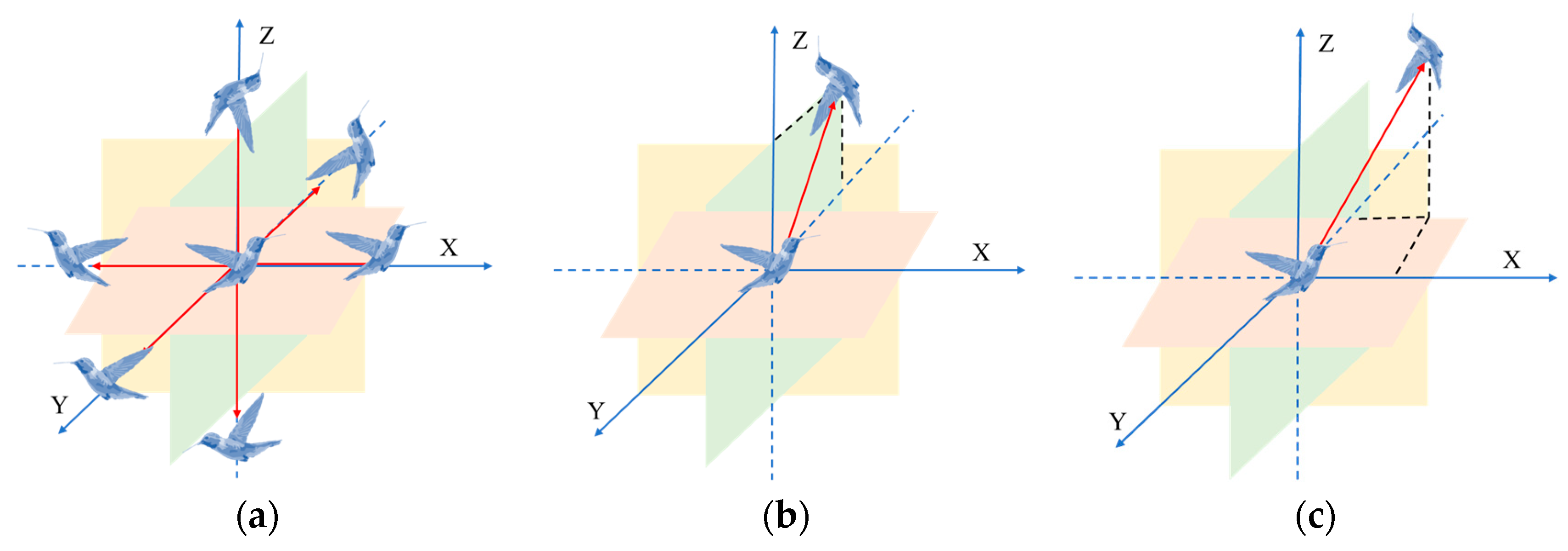
2.1.2. Guided Foraging
2.1.3. Territorial Foraging
2.1.4. Migration Foraging
2.2. Hybrid Artificial Hummingbird Algorithm
2.2.1. Elite Opposition-Based Learning
2.2.2. PSO Strategy
2.2.3. Cauchy Mutation Strategy
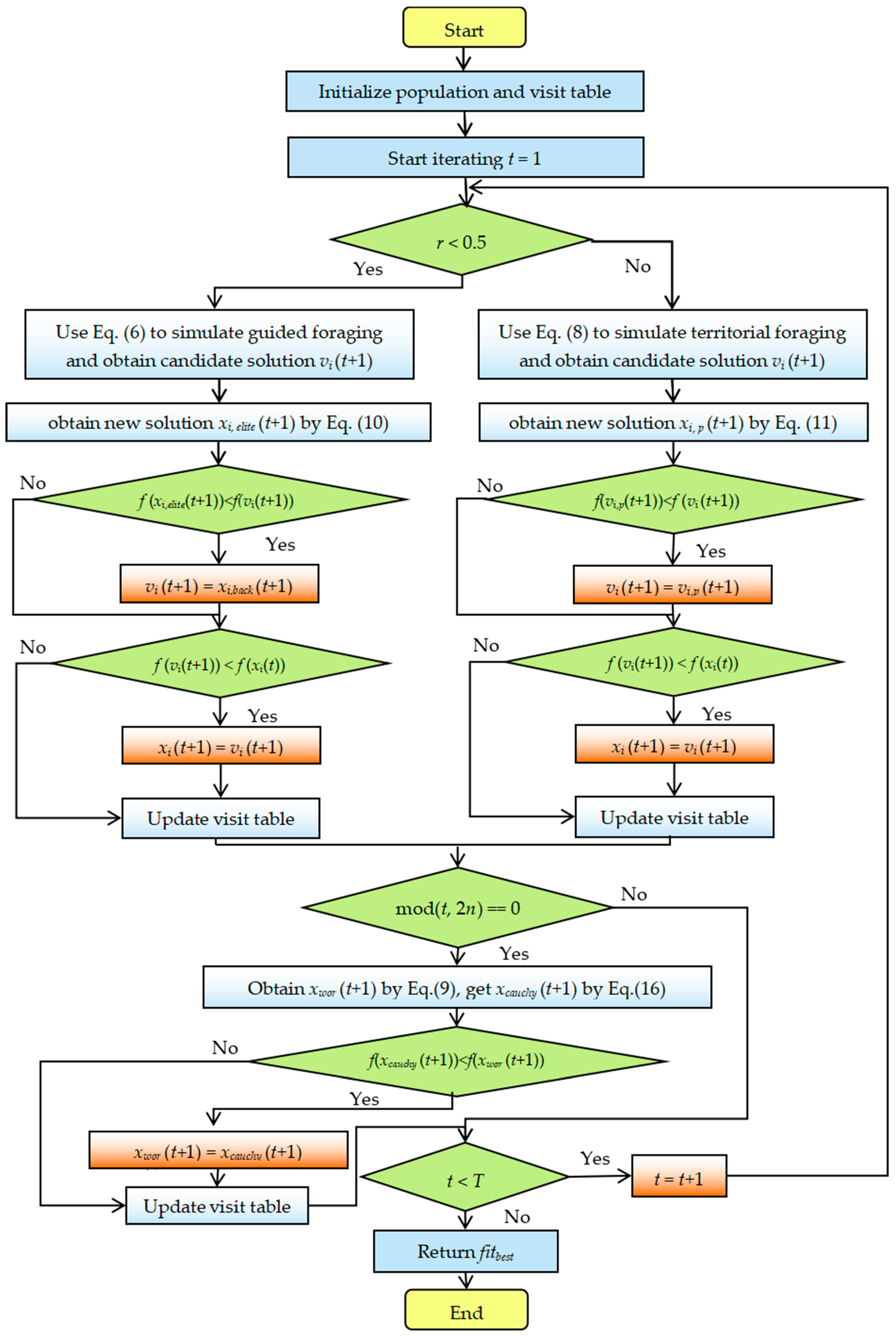
2.2.4. Detailed Steps for the Proposed HAHA
2.3. Computational Complexity of the Proposed HAHA
3. Numerical Experiments and Analysis
3.1. Benchmark Functions
3.2. Algorithm Parameter Settings
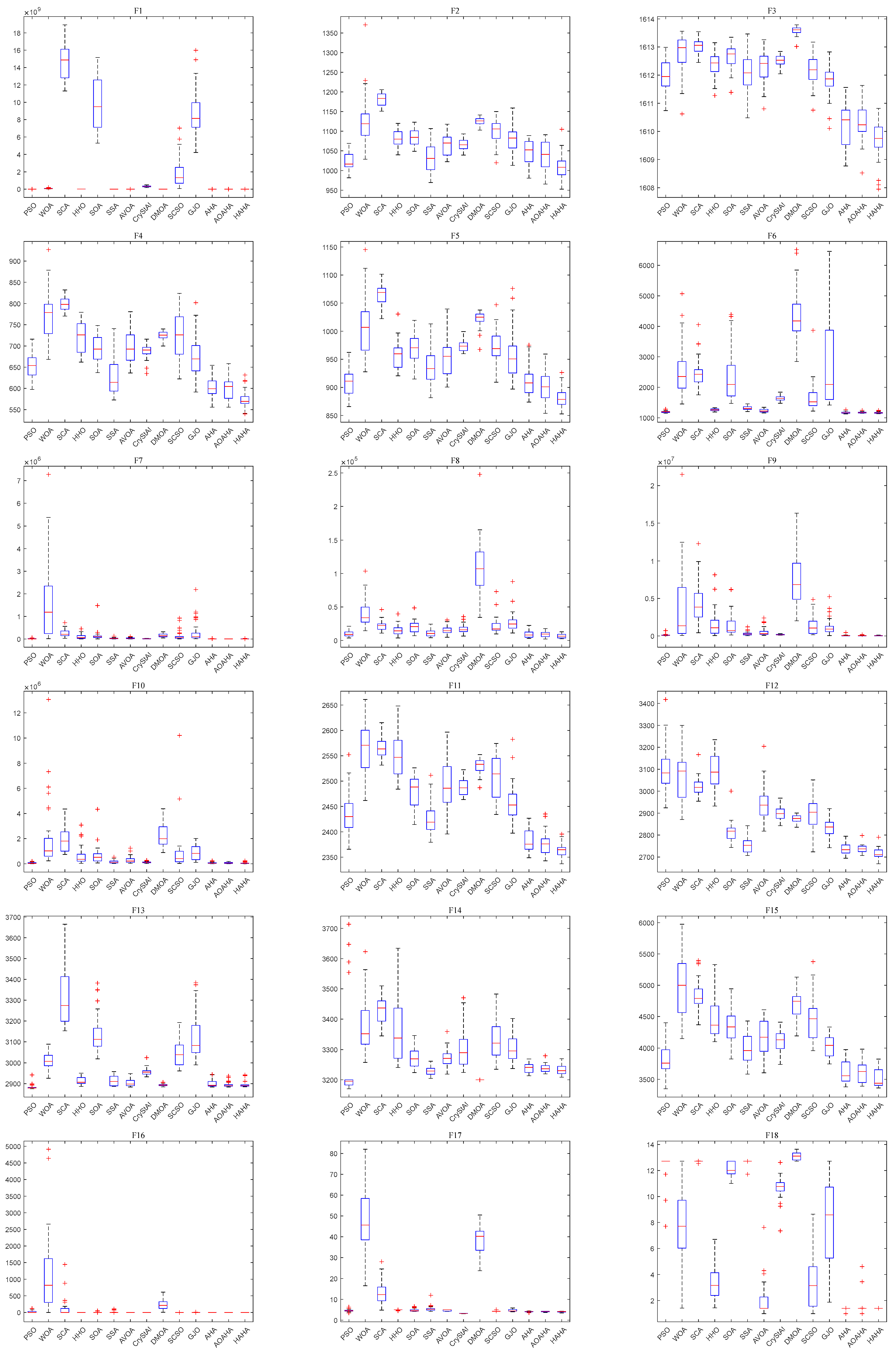
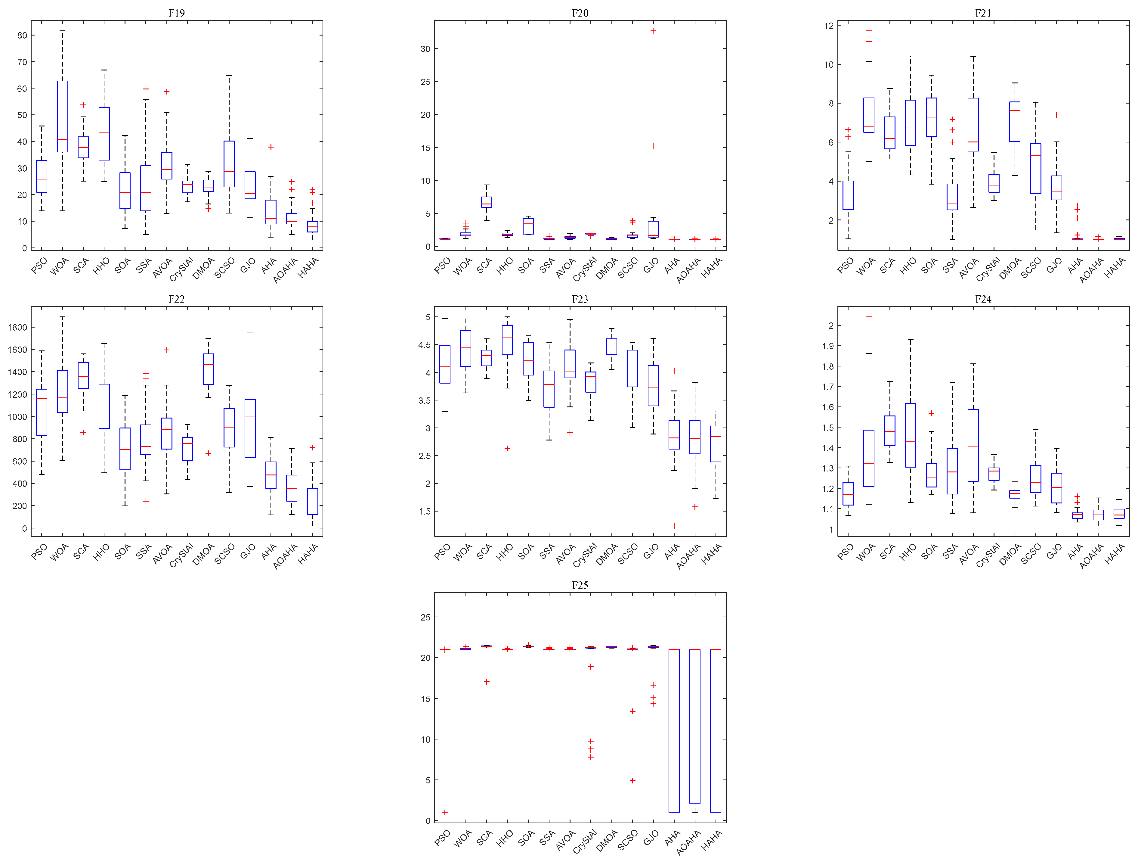
3.3. Results and Analyses for 25 Benchmark Functions
3.4. Results and Analyses on CEC 2022 Benchmark Functions
4. Construction of CSGC–Ball Curves
5. Application of HAHA in CSGC–Ball Curve-Shape Optimization
5.1. CSGC–Ball Curve-Shape Optimization Model
5.2. Steps for HAHA to Solve the CSGC–Ball Curve-Shape Optimization Model
5.3. Numerical Examples
6. Conclusions and Future Research
Author Contributions
Funding
Institutional Review Board Statement
Informed Consent Statement
Data Availability Statement
Conflicts of Interest
Appendix A. Twenty-Five Benchmark Functions
| Function Type | Function Name | Dim | Search Range | Optimal Value |
|---|---|---|---|---|
| Uni-modal functions | F1: Shifted and Rotated Bent Cigar Function (CEC 2017 F1) | 30 | [−100,100] | 100 |
| Multi-modal functions | F2: Shifted and Rotated Rastrigin’s Function (CEC 2014 F9) | 30 | [−100,100] | 900 |
| F3: Shifted and Rotated Expanded Scaffer’s F6 Function (CEC 2014 F16) | 30 | [−100,100] | 1600 | |
| F4: Shifted and Rotated Rastrigin’s Function (CEC 2017 F5) | 30 | [−100,100] | 500 | |
| F5: Shifted and Rotated Non-Continuous Rastrigin’s Function (CEC 2017 F8) | 30 | [−100,100] | 800 | |
| Hybrid functions | F6: Hybrid Function 1 (N = 3) (CEC 2017 F11) | 30 | [−100,100] | 1100 |
| F7: Hybrid Function 2 (N = 4) (CEC 2017 F14) | 30 | [−100,100] | 1400 | |
| F8: Hybrid Function 3 (N = 4) (CEC 2014 F20) | 30 | [−100,100] | 2000 | |
| F9: Hybrid Function 4 (N = 5) (CEC 2017 F18) | 30 | [−100,100] | 1800 | |
| F10: Hybrid Function 5 (N = 5) (CEC 2014 F21) | 30 | [−100,100] | 2100 | |
| Composition functions | F11: Composition Function 1 (N = 3) (CEC 2017 F21) | 30 | [−100,100] | 2100 |
| F12: Composition Function 2 (N = 4) (CEC 2017 F23) | 30 | [−100,100] | 2300 | |
| F13: Composition Function 3 (N = 5) (CEC 2017 F25) | 30 | [−100,100] | 2500 | |
| F14: Composition Function 4 (N = 6) (CEC 2017 F27) | 30 | [−100,100] | 2700 | |
| F15: Composition Function 5 (N = 3) (CEC 2017 F29) | 30 | [−100,100] | 2900 | |
| Fixed dimensional functions | F16: Storn’s Chebyshev Polynomial Fitting Problem (CEC 2019 F1) | 9 | [−8192,8192] | 1 |
| F17: Inverse Hilbert Matrix Problem (CEC 2019 F2) | 16 | [−16,384,16,384] | 1 | |
| F18: Lennard-Jones Minimum Energy Cluster (CEC 2019 F3) | 18 | [−4,4] | 1 | |
| F19: Rastrigin’s Function (CEC 2019 F4) | 10 | [−100,100] | 1 | |
| F20: Griewangk’s Function (CEC 2019 F5) | 10 | [−100,100] | 1 | |
| F21: Weierstrass Function (CEC 2019 F6) | 10 | [−100,100] | 1 | |
| F22: Modified Schwefel’s Function (CEC 2019 F7) | 10 | [−100,100] | 1 | |
| F23: Expanded Schaffer’s F6 Function (CEC 2019 F8) | 10 | [−100,100] | 1 | |
| F24: Happy Cat Function (CEC 2019 F9) | 10 | [−100,100] | 1 | |
| F25: Ackley Function (CEC 2019 F10) | 10 | [−100,100] | 1 |
Appendix B. Proof of Theorems in Section 4
Appendix B.1. Proof of Theorem 1
Appendix B.2. Proof of Theorem 2
Appendix C
| Algorithm | Optimal Shape Parameters | E | ||||||||
|---|---|---|---|---|---|---|---|---|---|---|
| PSO | 0.64887919 | 66.2849 | ||||||||
| j = 1 | j = 2 | j = 3 | j = 4 | j = 5 | j = 6 | j = 7 | j = 8 | |||
| 1.15185 | 1.37390 | 1.32772 | 1.55349 | 1.11589 | 1.29393 | 1.46232 | 1.54878 | |||
| 2.06512 | 1.96168 | 2.05905 | 1.80837 | 1.98417 | 1.64995 | 2.36528 | 1.96000 | |||
| 1.32390 | 1.28802 | 1.47045 | 1.45026 | 1.32576 | 1.06542 | 1.46548 | 1.16265 | |||
| WOA | 0.61246533 | 42.3460 | ||||||||
| j = 1 | j = 2 | j = 3 | j = 4 | j = 5 | j = 6 | j = 7 | j = 8 | |||
| 1.86538 | 2.53608 | 2.80315 | 2.74539 | 1.97669 | 2.50878 | 2.73656 | 2.61410 | |||
| 2.82767 | 2.10635 | 2.18380 | 2.26413 | 2.65508 | 2.20090 | 2.70274 | 2.71869 | |||
| 2.47729 | 2.63008 | 2.90391 | 2.23474 | 2.48893 | 2.59616 | 2.97236 | 2.24699 | |||
| SCA | 0.44943302 | 60.6286 | ||||||||
| j = 1 | j = 2 | j = 3 | j = 4 | j = 5 | j = 6 | j = 7 | j = 8 | |||
| 1.53812 | 1.21378 | 2.25093 | 1.89868 | 1.72244 | 1.40985 | 2.50022 | 2.24194 | |||
| 0.28967 | 0.22890 | 0.34591 | 0.12716 | 0.19957 | 0.37379 | 0.60330 | 0.37674 | |||
| 2.09452 | 2.25425 | 2.32298 | 2.21089 | 1.27993 | 2.21361 | 2.43706 | 1.85464 | |||
| HHO | 0.58330802 | 42.8444 | ||||||||
| j = 1 | j = 2 | j = 3 | j = 4 | j = 5 | j = 6 | j = 7 | j = 8 | |||
| 2.26112 | 2.66245 | 2.77293 | 2.75090 | 2.27722 | 2.72139 | 2.79630 | 2.64388 | |||
| 2.10014 | 2.04252 | 2.10340 | 2.23652 | 2.31288 | 2.04330 | 2.46973 | 2.39952 | |||
| 2.59681 | 2.71575 | 2.89981 | 2.36353 | 2.69098 | 2.67674 | 2.94551 | 2.39238 | |||
| GWO | 0.59802310 | 42.9182 | ||||||||
| j = 1 | j = 2 | j = 3 | j = 4 | j = 5 | j = 6 | j = 7 | j = 8 | |||
| 1.89364 | 2.73443 | 2.87954 | 2.83924 | 1.94839 | 2.80668 | 2.77928 | 2.63251 | |||
| 0.78809 | 0.87901 | 1.71278 | 1.69333 | 0.90586 | 0.45850 | 2.82386 | 0.49710 | |||
| 2.45587 | 2.61126 | 2.90566 | 2.20632 | 2.42842 | 2.42752 | 2.99789 | 2.28221 | |||
| HAHA | 0.77204510 | 41.7970 | ||||||||
| j = 1 | j = 2 | j = 3 | j = 4 | j = 5 | j = 6 | j = 7 | j = 8 | |||
| 1.72569 | 2.47537 | 2.45510 | 2.42984 | 1.76746 | 2.45557 | 2.36967 | 2.30659 | |||
| 1.96822 | 1.67667 | 2.11353 | 1.88233 | 2.03359 | 1.31535 | 2.71346 | 1.80763 | |||
| 2.23051 | 2.21689 | 2.53882 | 1.94375 | 2.27044 | 2.11102 | 2.64168 | 1.98074 | |||
Appendix D
| Algorithm | Optimal Shape Parameters | E | ||||||||
|---|---|---|---|---|---|---|---|---|---|---|
| PSO | 8.165946× 10⁻¹⁷ | 379.882 | ||||||||
| j = 1 | j = 2 | j = 3 | j = 4 | j = 5 | j = 6 | j = 7 | j = 8 | |||
| 0.01199 | 0.68281 | 0.37140 | −0.1024 | −0.3511 | 0.35437 | −0.3069 | −0.0002 | |||
| 1.90894 | 2.26708 | 2.15170 | 1.94534 | 1.88223 | 2.14267 | 1.77331 | 2.11611 | |||
| −0.1358 | 0.12068 | −0.1542 | 0.30099 | 0.33231 | 0.35239 | 0.12931 | −0.1755 | |||
| j = 9 | j = 10 | j =11 | j = 12 | j = 13 | j = 14 | j = 15 | j = 16 | |||
| −0.2375 | −0.1540 | −0.0842 | −0.0511 | 0.46105 | 0.25110 | 0.01922 | −0.1765 | |||
| 2.21089 | 1.87741 | 1.84059 | 1.92628 | 1.63868 | 2.20693 | 2.11329 | 1.87746 | |||
| 0.10939 | −0.1249 | −0.0502 | 0.24929 | −0.1074 | −0.0390 | 0.08777 | −0.1168 | |||
| j = 17 | j = 18 | j =19 | j = 20 | j = 21 | j = 22 | j = 23 | j = 24 | |||
| 0.04473 | −0.1061 | −0.0101 | 0.22035 | −0.2502 | 0.15433 | 0.17569 | −0.0559 | |||
| 1.99198 | 2.12004 | 2.12426 | 1.88229 | 1.90081 | 1.89130 | 1.87136 | 1.81734 | |||
| −0.0062 | 0.14957 | 0.17624 | 0.03901 | 0.01131 | −0.1524 | −0.1873 | 0.07681 | |||
| j = 25 | j = 26 | j =27 | j = 28 | j = 29 | ||||||
| 0.22829 | −0.2374 | 0.02877 | 0.18938 | 0.08976 | ||||||
| 1.96420 | 2.33591 | 2.08569 | 1.93850 | 1.98105 | ||||||
| 0.04001 | −0.1362 | −0.0880 | −0.1776 | 0.22704 | ||||||
| WOA | 0.56143072 | 184.656 | ||||||||
| j = 1 | j = 2 | j = 3 | j = 4 | j = 5 | j = 6 | j = 7 | j = 8 | |||
| 2.85218 | 2.87138 | 2.82369 | 2.89281 | 2.98078 | 2.83488 | 2.88864 | 2.86913 | |||
| 2.35992 | 2.05760 | 2.36563 | 1.84918 | 2.34436 | 2.21655 | 2.30250 | 2.16827 | |||
| 2.89427 | 2.90698 | 2.93313 | 2.81194 | 2.91938 | 2.87946 | 2.87397 | 2.86274 | |||
| j = 9 | j = 10 | j =11 | j = 12 | j = 13 | j = 14 | j = 15 | j = 16 | |||
| 2.87848 | 2.87460 | 2.84069 | 2.87111 | 2.86491 | 2.86395 | 2.86615 | 2.87630 | |||
| 2.16549 | 2.21958 | 2.33277 | 2.16387 | 1.82327 | 2.08353 | 2.14077 | 1.87726 | |||
| 2.85025 | 2.85099 | 2.89884 | 2.81336 | 2.85745 | 2.89370 | 2.89365 | 2.89385 | |||
| j = 17 | j = 18 | j =19 | j = 20 | j = 21 | j = 22 | j = 23 | j = 24 | |||
| 2.84521 | 2.85292 | 2.78854 | 2.84806 | 2.85620 | 2.82256 | 2.82369 | 2.81984 | |||
| 2.20087 | 2.39431 | 2.24645 | 2.64762 | 2.45415 | 2.27135 | 2.58449 | 2.39753 | |||
| 2.87404 | 2.88912 | 2.77618 | 2.85626 | 2.86230 | 2.89564 | 2.87897 | 2.87074 | |||
| j = 25 | j = 26 | j =27 | j = 28 | j = 29 | ||||||
| 2.78441 | 2.86354 | 2.86487 | 2.84957 | 2.85947 | ||||||
| 2.59021 | 2.35955 | 2.00985 | 2.34287 | 2.20680 | ||||||
| 2.84430 | 2.91575 | 2.87652 | 2.92195 | 2.86763 | ||||||
| SCA | 0.01240168 | 378.441 | ||||||||
| j = 1 | j = 2 | j = 3 | j = 4 | j = 5 | j = 6 | j = 7 | j = 8 | |||
| −1.0570 | −0.3385 | 0.23026 | 0.08677 | 0.60017 | −0.1256 | −0.5899 | −0.0320 | |||
| 2.15431 | 1.46926 | 1.64490 | 1.50380 | 2.03020 | 1.77393 | 1.23516 | 1.80551 | |||
| 0.52234 | 0.12062 | −0.4202 | −0.2678 | −0.4550 | −0.0387 | −0.2334 | −0.0960 | |||
| j = 9 | j = 10 | j =11 | j = 12 | j = 13 | j = 14 | j = 15 | j = 16 | |||
| 0.45369 | 0.01261 | −0.4439 | −0.1557 | −0.0764 | −0.0760 | −0.3289 | 0.17971 | |||
| 1.50170 | 1.45567 | 1.64068 | 1.91496 | 1.93461 | 2.28278 | 1.55732 | 1.72778 | |||
| −0.2907 | −0.2423 | 0.01349 | −0.3109 | −0.1890 | −0.2911 | −0.0978 | 0.77774 | |||
| j = 17 | j = 18 | j =19 | j = 20 | j = 21 | j = 22 | j = 23 | j = 24 | |||
| 0.49273 | 0.25800 | −0.1537 | −0.1686 | 0.12123 | −0.4168 | 0.51629 | 0.29765 | |||
| 1.49014 | 2.09171 | 1.38876 | 1.95450 | 1.95912 | 1.58009 | 1.86773 | 1.87182 | |||
| −0.0568 | 0.03448 | −0.1341 | 0.47338 | −0.8309 | −0.2569 | 0.12387 | −0.7595 | |||
| j = 25 | j = 26 | j =27 | j = 28 | j = 29 | ||||||
| 0.06529 | 0.53273 | 0.11868 | 0.01192 | −0.1921 | ||||||
| 1.53690 | 2.10757 | 1.98951 | 1.84692 | 2.61408 | ||||||
| −0.2140 | −0.2751 | 0.63215 | −0.3338 | −0.5503 | ||||||
| HHO | 0.53141245 | 184.025 | ||||||||
| j = 1 | j = 2 | j = 3 | j = 4 | j = 5 | j = 6 | j = 7 | j = 8 | |||
| 2.98076 | 2.98442 | 2.98010 | 2.97835 | 2.99602 | 2.98160 | 2.98318 | 2.97598 | |||
| 1.98222 | 2.00455 | 2.07102 | 2.00812 | 2.03681 | 1.99617 | 2.02540 | 1.98957 | |||
| 2.98414 | 2.99028 | 2.98943 | 2.98353 | 2.97914 | 2.98232 | 2.98244 | 2.98264 | |||
| j = 9 | j = 10 | j =11 | j = 12 | j = 13 | j = 14 | j = 15 | j = 16 | |||
| 2.98423 | 2.97553 | 2.97932 | 2.98584 | 2.98094 | 2.98193 | 2.98142 | 2.98279 | |||
| 1.92067 | 1.96532 | 2.05272 | 1.94200 | 1.98074 | 2.02657 | 2.03130 | 1.92533 | |||
| 2.97530 | 2.97999 | 2.98822 | 2.96541 | 2.97992 | 2.98762 | 2.98329 | 2.98282 | |||
| j = 17 | j = 18 | j =19 | j = 20 | j = 21 | j = 22 | j = 23 | j = 24 | |||
| 2.97561 | 2.98808 | 2.97989 | 2.98418 | 2.97869 | 2.98229 | 2.97976 | 2.98119 | |||
| 2.05583 | 2.06593 | 2.02464 | 1.99876 | 1.95430 | 1.96503 | 1.98384 | 1.95259 | |||
| 2.98265 | 2.98353 | 2.98228 | 2.98389 | 2.98242 | 2.98294 | 2.98386 | 2.98094 | |||
| j = 25 | j = 26 | j =27 | j = 28 | j = 29 | ||||||
| 2.98291 | 2.98321 | 2.98492 | 2.98132 | 2.97698 | ||||||
| 1.99819 | 1.99420 | 2.01433 | 1.95868 | 2.06611 | ||||||
| 2.97534 | 2.98722 | 2.97132 | 2.98569 | 2.98160 | ||||||
| SMA | 0.85577335 | 208.323 | ||||||||
| j = 1 | j = 2 | j = 3 | j = 4 | j = 5 | j = 6 | j = 7 | j = 8 | |||
| 2.13464 | 2.13464 | 2.13464 | 2.13464 | 2.13464 | 2.13464 | 2.13464 | 2.13464 | |||
| 3.42309 | 3.42309 | 3.42309 | 3.42309 | 3.42309 | 3.42309 | 3.42309 | 3.42309 | |||
| 2.13464 | 2.13464 | 2.13464 | 2.13464 | 2.13464 | 2.13464 | 2.13464 | 2.13464 | |||
| j = 9 | j = 10 | j =11 | j = 12 | j = 13 | j = 14 | j = 15 | j = 16 | |||
| 2.13464 | 2.13464 | 2.13464 | 2.13464 | 2.13464 | 2.13464 | 2.13464 | 2.13464 | |||
| 3.42309 | 3.42309 | 3.42309 | 3.42309 | 3.42309 | 3.42309 | 3.42309 | 3.42309 | |||
| 2.13464 | 2.13464 | 2.13464 | 2.13464 | 2.13464 | 2.13464 | 2.13464 | 2.13464 | |||
| j = 17 | j = 18 | j =19 | j = 20 | j = 21 | j = 22 | j = 23 | j = 24 | |||
| 2.13464 | 2.13464 | 2.13464 | 2.13464 | 2.13464 | 2.13464 | 2.13464 | 2.13464 | |||
| 3.42309 | 3.42309 | 3.42309 | 3.42309 | 3.42309 | 3.42309 | 3.42309 | 3.42309 | |||
| 2.13464 | 2.13464 | 2.13464 | 2.13464 | 2.13464 | 2.13464 | 2.13464 | 2.13464 | |||
| j = 25 | j = 26 | j =27 | j = 28 | j = 29 | ||||||
| 2.13464 | 2.13464 | 2.13464 | 2.13464 | 2.13464 | ||||||
| 3.42309 | 3.42309 | 3.42309 | 3.42309 | 3.42309 | ||||||
| 2.13464 | 2.13464 | 2.13464 | 2.13464 | 2.13464 | ||||||
| HAHA | 0.75838681 | 182.437 | ||||||||
| j = 1 | j = 2 | j = 3 | j = 4 | j = 5 | j = 6 | j = 7 | j = 8 | |||
| 2.32285 | 2.39393 | 2.24157 | 2.38538 | 2.74613 | 2.39668 | 2.35229 | 2.37876 | |||
| 2.07657 | 1.87513 | 2.00551 | 1.06112 | 1.47205 | 1.90181 | 2.12946 | 1.97447 | |||
| 2.44915 | 2.49225 | 2.59108 | 1.58380 | 1.73668 | 2.31265 | 2.42312 | 2.34776 | |||
| j = 9 | j = 10 | j =11 | j = 12 | j = 13 | j = 14 | j = 15 | j = 16 | |||
| 2.38142 | 2.33024 | 2.36332 | 2.38664 | 2.41047 | 2.37189 | 2.35745 | 2.41375 | |||
| 1.96577 | 2.14084 | 2.09773 | 1.88414 | 1.75302 | 1.95039 | 2.08764 | 1.71225 | |||
| 2.31657 | 2.29552 | 2.38640 | 2.25331 | 2.33960 | 2.41308 | 2.41769 | 2.36731 | |||
| j = 17 | j = 18 | j =19 | j = 20 | j = 21 | j = 22 | j = 23 | j = 24 | |||
| 2.35154 | 2.21571 | 2.36552 | 2.40253 | 2.31975 | 2.32859 | 2.27686 | 2.39248 | |||
| 2.13212 | 2.97383 | 1.95326 | 1.86995 | 2.30571 | 2.34025 | 2.44898 | 1.85148 | |||
| 2.36369 | 2.82544 | 2.29492 | 2.40542 | 2.37088 | 2.68900 | 2.42857 | 2.40000 | |||
| j = 25 | j = 26 | j =27 | j = 28 | j = 29 | ||||||
| 2.27982 | 2.28423 | 2.40584 | 2.33562 | 2.29302 | ||||||
| 2.45719 | 2.76197 | 1.53374 | 2.27599 | 2.09232 | ||||||
| 2.34878 | 2.60824 | 2.26335 | 2.67179 | 2.43301 | ||||||
References
- Shi, F.Z. Computer Aided Geometric Design and Nonuniform Rational B-Splines: CAGD & NURBS; Beijing University of Aeronautics and Astronautics Press: Beijing, China, 2001. [Google Scholar]
- Wang, G.J.; Wang, G.Z.; Zheng, J.M. Computer Aided Geometric Design; Higher Education Press: Beijing, China, 2001. [Google Scholar]
- Hu, G.; Dou, W.T.; Wang, X.F.; Abbas, M. An enhanced chimp optimization algorithm for optimal degree reduction of Said–Ball curves. Math. Comput. Simul. 2022, 197, 207–252. [Google Scholar] [CrossRef]
- Consurf, A.A. Part one: Introduction of the conic lofting tile. Comput.-Aided Des. 1974, 6, 243–249. [Google Scholar]
- Wang, G.J. Ball curve of high degree and its geometric properties. Appl. Math. A J. Chin. Univ. 1987, 2, 126–140. [Google Scholar]
- Said, H.B. A generalized ball curve and its recursive algorithm. ACM Trans. Graph. (TOG) 1989, 8, 360–371. [Google Scholar] [CrossRef]
- Hu, S.M.; Wang, G.Z.; Jin, T.G. Properties of two types of generalized Ball curves. Comput.-Aided Des. 1996, 28, 125–133. [Google Scholar] [CrossRef]
- Othlnan, W.; Goldman, R.N. The dual basis functions for the generalized ball basis of odd degree. Comput. Aided Geom. Des. 1997, 14, 571–582. [Google Scholar]
- Xi, M.C. Dual basis of Ball basis function and its application. Comput. Math. 1997, 19, 7. [Google Scholar]
- Ding, D.Y.; Li, M. Properties and applications of generalized Ball curves. Chin. J. Appl. Math. 2000, 23, 123–131. [Google Scholar]
- Jiang, P.; Wu, H. Dual basis of Wang-Ball basis function and its application. J. Comput. Aided Des. Graph. 2004, 16, 454–458. [Google Scholar]
- Hu, S.M.; Jin, T.G. Degree reductive approximation of Bézier curves. In Proceedings of the Eighth Annual Symposium on Computational Geometry, Berlin, Germany, 10–12 June 1992; pp. 110–126. [Google Scholar]
- Wu, H.Y. Two new kinds of generalized Ball curves. J. Appl. Math. 2000, 23, 196–205. [Google Scholar]
- Wang, C.W. Extension of cubic Ball curve. J. Eng. Graph. 2008, 29, 77–81. [Google Scholar]
- Wang, C.W. The extension of the quartic Wang-Ball curve. J. Eng. Graph. 2009, 30, 80–84. [Google Scholar]
- Yan, L.L.; Zhang, W.; Wen, R.S. Two types of shape-adjustable fifth-order generalized Ball curves. J. Eng. Graph. 2011, 32, 16–20. [Google Scholar]
- Hu, G.S.; Wang, D.; Yu, A.M. Construction and application of 2m+2 degree Ball curve with shape parameters. J. Eng. Graph. 2009, 30, 69–79. [Google Scholar]
- Xiong, J.; Guo, Q.W. Generalized Wang-Ball curve. Numer. Comput. Comput. Appl. 2013, 34, 187–195. [Google Scholar]
- Liu, H.Y.; Li, L.; Zhang, D.M. Quadratic Ball curve with shape parameters. J. Shandong Univ. 2011, 41, 23–28. [Google Scholar]
- Huang, C.L.; Huang, Y.D. Quartic Wang-Ball curve and surface with two parameters. J. Hefei Univ. Technol. 2012, 35, 1436–1440. [Google Scholar]
- Hu, G.; Zhu, X.N.; Wei, G.; Chang, C.T. An improved marine predators algorithm for shape optimization of developable Ball surfaces. Eng. Appl. Artif. Intell 2021, 105, 104417. [Google Scholar] [CrossRef]
- Hu, G.; Li, M.; Wang, X.; Wei, G.; Chang, C.T. An enhanced manta ray foraging optimization algorithm for shape optimization of complex CCG-Ball curves. Knowl. Based Syst. 2022, 240, 108071. [Google Scholar] [CrossRef]
- Gurunathan, B.; Dhande, S. Algorithms for development of certain classes of ruled surfaces. Comput. Graph 1987, 11, 105–112. [Google Scholar] [CrossRef]
- Jaklič, G.; Žagar, E. Curvature variation minimizing cubic Hermite interpolants. Appl. Math. Comput. 2011, 218, 3918–3924. [Google Scholar] [CrossRef]
- Lu, L.Z. A note on curvature variation minimizing cubic Hermite interpolants. Appl. Math. Comput. 2015, 259, 596–599. [Google Scholar] [CrossRef]
- Zheng, J.Y.; Hu, G.; Ji, X.M.; Qin, X.Q. Quintic generalized Hermite interpolation curves: Construction and shape optimization using an improved GWO algorithm. Comput. Appl. Math 2022, 41, 115. [Google Scholar] [CrossRef]
- Hu, G.; Wu, J.L.; Li, H.N.; Hu, X.Z. Shape optimization of generalized developable H-Bézier surfaces using adaptive cuckoo search algorithm. Adv. Eng. Softw. 2020, 149, 102889. [Google Scholar] [CrossRef]
- Ahmadianfar, I.; Heidari, A.; Gandomi, A.H.; Chu, X.; Chen, H. RUN beyond the metaphor: An efficient optimization algorithm based on Runge Kutta method. Expert Syst. Appl. 2021, 181, 115079. [Google Scholar] [CrossRef]
- Hu, G.; Du, B.; Wang, X.F.; Wei, G. An enhanced black widow optimization algorithm for feature selection. Knowl. Based Syst. 2022, 35, 107638. [Google Scholar] [CrossRef]
- Wolpert, D.H.; Macready, W.G. No free lunch theorems for optimization. IEEE Trans. Evol. Comput. 1997, 1, 67–82. [Google Scholar] [CrossRef]
- Nematollahi, A.F.; Rahiminejad, A.; Vahidi, B. A novel meta-heuristic optimization method based on golden ratio in nature. Soft Comput. 2020, 24, 1117–1151. [Google Scholar] [CrossRef]
- Holland, J.H. Genetic algorithms. Sci. Am. 1992, 267, 66–72. [Google Scholar] [CrossRef]
- Storn, R.; Price, K. Differential evolution–a simple and efficient heuristic for global optimization over continuous Spaces. J. Glob. Optim. 1997, 11, 341–359. [Google Scholar] [CrossRef]
- Koza, J.R. Genetic Programming: On the Programming of Computers by Means of Natural Selection; MIT Press: Cambridge, MA, USA, 1992. [Google Scholar]
- Li, W.Z.; Wang, L.; Cai, X.; Hu, J.; Guo, W. Species co-evolutionary algorithm: A novel evolutionary algorithm based on the ecology and environments for optimization. Neural. Comput. Appl. 2019, 31, 2015–2024. [Google Scholar] [CrossRef]
- Kirkpatrick, S.; Gelatt, C.D.; Vecchi, M.P. Optimization by simulated annealing. Science 1983, 220, 671–680. [Google Scholar] [CrossRef] [PubMed]
- Rashedi, E.; Nezamabadi-Pour, H.; Saryazdi, S. GSA: A gravitational search algorithm. Inf. Sci. 2009, 179, 2232–2248. [Google Scholar] [CrossRef]
- Mirjalili, S. SCA: A Sine Cosine Algorithm for Solving Optimization Problems. Knowl. Based Syst. 2016, 96, 120–133. [Google Scholar] [CrossRef]
- Hashim, F.A.; Hussain, K.; Houssein, E.H.; Mai, S.M.; Al-Atabany, W. Archimedes optimization algorithm: A new metaheuristic algorithm for solving optimization problems. Appl. Intell. 2020, 51, 1531–1551. [Google Scholar] [CrossRef]
- Talatahari, S.; Azizi, M.; Tolouei, M.; Talatahari, B.; Sareh, P. Crystal structure algorithm (CryStAl): A metaheuristic optimization method. IEEE Access 2021, 9, 71244–71261. [Google Scholar] [CrossRef]
- Salawudeen, A.T.; Mu’Azu, M.B.; Sha’Aban, Y.A.; Adedokun, A.E. A novel smell agent optimization (sao): An extensive cec study and engineering application. Knowl. Based Syst. 2021, 232, 107486. [Google Scholar] [CrossRef]
- Rao, R.V.; Savsani, V.J.; Vakharia, D.P. Teaching-Learning-Based Optimization: An optimization method for continuous non-linear large scale problems. Inf. Sci. 2012, 183, 1–15. [Google Scholar] [CrossRef]
- Satapathy, S.; Naik, A. Social group optimization (SGO): A new population evolutionary optimization technique. Complex Intell. Syst. 2016, 2, 173–203. [Google Scholar] [CrossRef]
- Bikash, D.; Mukherjee, V.; Debapriya, D. Student psychology based optimization algorithm: A new population based optimization algorithm for solving optimization problems. Adv. Eng. Softw. 2020, 146, 102804. [Google Scholar]
- Bodaghi, M.; Samieefar, K. Meta-heuristic bus transportation algorithm. Iran J. Comput. Sci. 2019, 2, 23–32. [Google Scholar] [CrossRef]
- Yuan, Y.L.; Ren, J.J.; Wang, S.; Wang, Z.X.; Mu, X.K.; Zhao, W. Alpine skiing optimization: A new bio-inspired optimization algorithm. Adv. Eng. Softw. 2022, 170, 103158. [Google Scholar] [CrossRef]
- Kennedy, J.; Eberhart, R. Particle swarm optimization. In Proceedings of the ICNN’95-International Conference on NeuralNetworks, Perth, Australia, 27 November–1 December 1995; pp. 1942–1948. [Google Scholar]
- Dorigo, M.; Blum, C. Ant colony optimization theory: A survey. Theor. Comput. Sci. 2005, 344, 243–278. [Google Scholar] [CrossRef]
- Mirjalili, S. Moth-flame optimization algorithm: A novel nature-inspired heuristic paradigm. Knowl. Based Syst. 2015, 89, 228–249. [Google Scholar] [CrossRef]
- Ma, L.; Wang, C.; Xie, N.G.; Shi, M.; Wang, L. Moth-flame optimization algorithm based on diversity and mutation strategy. Appl. Intell. 2021, 51, 5836–5872. [Google Scholar] [CrossRef]
- Wang, C.; Ma, L.L.; Ma, L.; Lai, J.; Zhao, J.; Wang, L.; Cheong, K.H. Identification of influential users with cost minimization via an improved moth flame optimization. J. Comput. Sci. 2023, 67, 101955. [Google Scholar] [CrossRef]
- Mirjalili, S.; Mirjalili, S.M.; Lewis, A. Grey Wolf Optimizer. Adv. Eng. Softw. 2014, 69, 46–61. [Google Scholar] [CrossRef]
- Mirjalili, S.; Lewis, A. The whale optimization algorithm. Adv. Eng. Softw. 2016, 95, 51–67. [Google Scholar] [CrossRef]
- Heidari, A.A.; Mirjalili, S.; Faris, H.; Aljarah, I.; Mafarja, M.; Chen, H.L. Harris hawks optimization: Algorithm and applications. Future Gener. Comput. Syst. 2019, 97, 849–872. [Google Scholar] [CrossRef]
- Hayyolalam, V.; Kazem, A.A.P. Black Widow Optimization Algorithm: A novel meta-heuristic approach for solving engineering optimization problems. Eng. Appl. Artif. Intell. 2020, 87, 103249. [Google Scholar] [CrossRef]
- Huang, Q.H.; Wang, C.; Yılmaz, Y.; Wang, L.; Xie, N.G. Recognition of EEG based on Improved Black Widow Algorithm optimized SVM. Biomed. Signal Process Control 2023, 81, 104454. [Google Scholar] [CrossRef]
- Dhiman, G.; Kumar, V. Seagull optimization algorithm: Theory and its applications for large-scale industrial engineering problems. Knowl. Based Syst. 2019, 165, 169–196. [Google Scholar] [CrossRef]
- Mirjalili, S.; Gandomi, A.H.; Mirjalili, S.Z.; Saremi, S.; Faris, H.; Mirjalili, S.M. Salp swarm algorithm: A bio-inspired optimizer for engineering design problems. Adv. Eng. Softw. 2017, 114, 163–191. [Google Scholar] [CrossRef]
- Wang, C.; Xu, R.Q.; Ma, L.; Zhao, J.; Wang, L.; Xie, N.G. An efficient salp swarm algorithm based on scale-free informed followers with self-adaption weight. Appl. Intell. 2023, 53, 1759–1791. [Google Scholar] [CrossRef]
- Abdollahzadeh, B.; Gharehchopogh, F.S.; Mirjalili, S. African vultures optimization algorithm: A new nature-Inspired metaheuristic algorithm for global optimization problems. Comput. Ind. Eng. 2021, 158, 107408. [Google Scholar] [CrossRef]
- Agushaka, J.O.; Ezugwu, A.E.; Abualigah, L. Dwarf mongoose optimization algorithm. Comput. Methods Appl. Mech. Eng. 2022, 391, 114570. [Google Scholar] [CrossRef]
- Trojovský, P.; Dehghani, M. Pelican Optimization Algorithm: A Novel Nature-Inspired Algorithm for Engineering Applications. Sensors 2022, 22, 855. [Google Scholar] [CrossRef]
- Nitish, C.; Muhammad, M.A. Golden jackal optimization: A novel nature-inspired optimizer for engineering applications. Expert Syst. Appl. 2022, 198, 116924. [Google Scholar]
- Zhao, W.; Wang, L.; Mirjalili, S. Artificial hummingbird algorithm: A new bio-inspired optimizer with its engineering applications. Comput. Methods Appl. Mech. Eng. 2022, 388, 114194. [Google Scholar] [CrossRef]
- Ramadan, A.; Kamel, S.; Hassan, M.H.; Ahmed, E.M.; Hasanien, H.M. Accurate photovoltaic models based on an adaptive opposition artificial hummingbird algorithm. Electronics 2022, 11, 318. [Google Scholar] [CrossRef]
- Mohamed, H.; Ragab, E.S.; Ahmed, G.; Ehab, E.; Abdullah, S. Parameter identification and state of charge estimation of Li-Ion batteries used in electric vehicles using artificial hummingbird optimizer. J. Energy Storage 2022, 51, 104535. [Google Scholar]
- Sadoun, A.M.; Najjar, I.R.; Alsoruji, G.S.; Abd-Elwahed, M.S.; Elaziz, M.A.; Fathy, A. Utilization of improved machine learning method based on artificial hummingbird algorithm to predict the tribological Behavior of Cu-Al2O3 nanocomposites synthesized by In Situ method. Mathematics 2022, 10, 1266. [Google Scholar] [CrossRef]
- Abid, M.S.; Apon, H.J.; Morshed, K.A.; Ahmed, A. Optimal planning of multiple renewable energy-integrated distribution system with uncertainties using artificial hummingbird algorithm. IEEE Access 2022, 10, 40716–40730. [Google Scholar] [CrossRef]
- Yildiz, B.S.; Pholdee, N.; Bureerat, S.; Yildiz, A.; Sait, S. Enhanced grasshopper optimization algorithm using elite opposition-based learning for solving real-world engineering problems. Eng. Comput. 2021, 38, 4207–4219. [Google Scholar] [CrossRef]
- Wang, Y.J.; Su, T.T.; Liu, L. Multi-strategy cooperative evolutionary PSO based on Cauchy mutation strategy. J. Syst. Simul. 2018, 30, 2875–2883. [Google Scholar]
- Hu, G.; Chen, L.X.; Wang, X.P.; Guo, W. Differential Evolution-Boosted Sine Cosine Golden Eagle Optimizer with Lévy Flight. J. Bionic. Eng. 2022, 19, 850–1885. [Google Scholar] [CrossRef]
- Seyyedabbasi, A.; Kiani, F. Sand Cat swarm optimization: A nature-inspired algorithm to solve global optimization problems. Eng. Comput. 2022, 39, 2627–2651. [Google Scholar] [CrossRef]
- Hu, G.; Zhong, J.Y.; Du, B.; Guo, W. An enhanced hybrid arithmetic optimization algorithm for engineering applications. Comput. Methods Appl. Mech. Eng. 2022, 394, 114901. [Google Scholar] [CrossRef]
- Wilcoxon, F.; Bulletin, S.B.; Dec, N. Individual Comparisons by Ranking Methods; Springer: New York, NY, USA, 1992. [Google Scholar]
- Derrac, J.; García, S.; Molina, D.; Herrera, F. A practical tutorial on the use of nonparametric statistical tests as a methodology for comparing evolutionary and swarm intelligence algorithms. Swarm Evol. Comput. 2011, 1, 3–18. [Google Scholar] [CrossRef]
- Mohamed, A.; Reda, M.; Shaimaa, A.A.A.; Mohammed, J.; Mohamed, A. Kepler optimization algorithm: A new metaheuristic algorithm inspired by Kepler’s laws of planetary motion. Knowl. Based Syst. 2023, 268, 110454. [Google Scholar]
- Li, S.M.; Chen, H.L.; Wang, M.J.; Heidari, A.; Mirjalili, S. Slime mould algorithm: A new method for stochastic optimization. Future Gener. Comput. Syst. 2022, 111, 300–323. [Google Scholar] [CrossRef]
- Zheng, J.; Ji, X.; Ma, Z.; Hu, G. Construction of Local-Shape-Controlled Quartic Generalized Said-Ball Model. Mathematics 2023, 11, 2369. [Google Scholar] [CrossRef]
- Hu, G.; Wang, J.; Li, M.; Hussien, A.G.; Abbas, M. EJS: Multi-strategy enhanced jellyfish search algorithm for engineering applications. Mathematics 2023, 11, 851. [Google Scholar] [CrossRef]
- Hu, G.; Zhong, J.; Wei, G.; Chang, C.-T. DTCSMO: An efficient hybrid starling murmuration optimizer for engineering applications, Comput. Methods Appl. Mech. Eng. 2023, 405, 115878. [Google Scholar] [CrossRef]
- Hu, G.; Yang, R.; Qin, X.Q.; Wei, G. MCSA: Multi-strategy boosted chameleon-inspired optimization algorithm for engineering applications. Comput. Methods Appl. Mech. Eng. 2023, 403, 115676. [Google Scholar] [CrossRef]


| Algorithm | Parameters | Setting Value |
|---|---|---|
| All algorithm | Population size (n) | 100 |
| Max iterations (T) | 1000 | |
| Number of runs | 30 | |
| AHA | Migration coefficient (M) | 2n |
| HAHA | Learning factors (c1, c2) | 2 |
| Migration coefficient (M) | 2n | |
| PSO | Neighboring ratio | 0.25 |
| Inertia weight (ω) | 0.9 | |
| Cognitive and social factors | c1 = c2 = 1.5 | |
| WOA | Parameter (a) | from 2 to 0 |
| SCA | Constant (a) | 2 |
| HHO | Energy (E1) | from 2 to 0 |
| SOA | Control factor (fc) | 2 |
| AOA | C3, C4 | C3 = 1,C4 = 2 |
| GJO | Decreasing energy of the prey (E1) | from 1.5 to 0 |
| Constant values (β, c1) | 1.5, 1.5 | |
| POA | R | 0.2 |
| SCSO | Sensitivity range (rG) | from 2 to 0 |
| R | from −2rG to 2rG | |
| KOA | , μ0, γ | 3, 0.1, 15 |
| F | Index | Algorithms | |||||||||||||
|---|---|---|---|---|---|---|---|---|---|---|---|---|---|---|---|
| PSO | WOA | SCA | HHO | SOA | SSA | AVOA | CryStAl | DMOA | SCSO | GJO | AHA | AOAHA | HAHA | ||
| F1 | Avg. | 2.29 × 10³ | 6.75 × 10⁷ | 1.46 × 10¹⁰ | 1.21 × 10⁷ | 9.84 × 10⁹ | 5.35 × 10³ | 4.04 × 10³ | 3.11 × 10⁸ | 4.40 × 10⁶ | 2.05 × 10⁹ | 8.79 × 10⁹ | 4.87 × 10³ | 3.12 × 10³ | 1.64 ×10³ |
| Std. | 3.60 × 10³ | 3.95 × 10⁷ | 2.15 × 10⁹ | 2.42 × 10⁶ | 2.89 × 10⁹ | 5.89 × 10³ | 4.80 × 10³ | 7.57 × 10⁷ | 2.91 × 10⁶ | 1.87 × 10⁹ | 2.68 × 10⁹ | 6.17 × 10³ | 3.58 × 10³ | 1.94 × 10³ | |
| p-value | 0.185767 | 3.02 × 10⁻¹¹ | 3.02 × 10⁻¹¹ | 3.02 × 10⁻¹¹ | 3.02 × 10⁻¹¹ | 3.67 × 10⁻³ | 1.49 × 10⁻¹ | 3.02 × 10⁻¹¹ | 3.02 × 10⁻¹¹ | 3.02 × 10⁻¹¹ | 3.02 × 10⁻¹¹ | 0.001370 | 0.036439 | \ | |
| Rank | 2 | 9 | 14 | 8 | 13 | 6 | 4 | 10 | 7 | 11 | 12 | 5 | 3 | 1 | |
| F2 | Avg. | 1.02 × 10³ | 1.13 × 10³ | 1.18 × 10³ | 1.08 × 10³ | 1.08 × 10³ | 1.03 × 10³ | 1.07 × 10³ | 1.07 × 10³ | 1.12 × 10³ | 1.10 × 10³ | 1.08 × 10³ | 1.05 × 10³ | 1.04 × 10³ | 1.01 × 10³ |
| Std. | 24.2 | 65.4 | 16.5 | 20.6 | 22 | 38.6 | 27.9 | 12.4 | 10.5 | 30.3 | 37 | 29.2 | 37.6 | 35.3 | |
| p-value | 0.133454 | 4.20 × 10⁻¹⁰ | 3.02 × 10⁻¹¹ | 2.67 × 10⁻⁹ | 1.69 × 10⁻⁹ | 5.55 × 10⁻² | 1.60 × 10⁻⁷ | 1.56 × 10⁻⁸ | 3.69 × 10⁻¹¹ | 1.07 × 10⁻⁹ | 5.53 × 10⁻⁸ | 6.36 × 10⁻⁵ | 0.009468 | \ | |
| Rank | 2 | 13 | 14 | 8 | 10 | 3 | 6 | 7 | 12 | 11 | 9 | 5 | 4 | 1 | |
| F3 | Avg. | 1611.994 | 1612.794 | 1613.027 | 1612.368 | 1612.638 | 1612.121 | 1612.296 | 1612.512 | 1613.589 | 1612.173 | 1611.799 | 1610.274 | 1610.294 | 1609.722 |
| Std. | 0.572 | 0.677 | 0.248 | 0.483 | 0.515 | 0.585 | 0.564 | 0.205 | 0.152 | 0.554 | 0.599 | 0.7471 | 0.624 | 0.710 | |
| p-value | 3.34 × 10⁻¹¹ | 3.69 × 10⁻¹¹ | 3.02 × 10⁻¹¹ | 3.02 × 10⁻¹¹ | 3.02 × 10⁻¹¹ | 4.50 × 10⁻¹¹ | 3.34 × 10⁻¹¹ | 3.02 × 10⁻¹¹ | 3.02 × 10⁻¹¹ | 3.34 × 10⁻¹¹ | 9.92 × 10⁻¹¹ | 0.011711 | 0.001236 | \ | |
| Rank | 5 | 12 | 13 | 9 | 11 | 6 | 8 | 10 | 14 | 7 | 4 | 2 | 3 | 1 | |
| F4 | Avg. | 653.6209 | 773.0286 | 798.6650 | 723.8702 | 694.3867 | 627.5682 | 698.6022 | 686.8479 | 725.0058 | 726.1686 | 674.7303 | 604.0870 | 599.1974 | 574.0913 |
| Std. | 28.5 | 60.2 | 17.3 | 37.6 | 31.6 | 44.8 | 38.2 | 16.9 | 9.40 | 50.7 | 47.7 | 24.1 | 24.4 | 22.6 | |
| p-value | 1.96 × 10⁻¹⁰ | 3.02 × 10⁻¹¹ | 3.02 × 10⁻¹¹ | 3.02 × 10⁻¹¹ | 3.02 × 10⁻¹¹ | 2.38 × 10⁻⁷ | 3.02 × 10⁻¹¹ | 3.02 × 10⁻¹¹ | 3.02 × 10⁻¹¹ | 3.34 × 10⁻¹¹ | 1.33 × 10⁻¹⁰ | 1.09 × 10⁻⁵ | 2.53 × 10⁻⁴ | \ | |
| Rank | 5 | 13 | 14 | 10 | 8 | 4 | 9 | 7 | 11 | 12 | 6 | 3 | 2 | 1 | |
| F5 | Avg. | 909.8099 | 1008.153 | 1066.307 | 957.5451 | 969.0228 | 939.2126 | 956.6075 | 973.4062 | 1020.7300 | 974.4398 | 959.1655 | 909.8768 | 899.4413 | 882.7806 |
| Std. | 23.6 | 49.1 | 17.8 | 23.2 | 26.1 | 34.9 | 34.8 | 9.56 | 14.7 | 29.1 | 46.3 | 24.4 | 25 | 17.4 | |
| p-value | 2.00 × 10⁻⁵ | 3.02 × 10⁻¹¹ | 3.02 × 10⁻¹¹ | 3.69 × 10⁻¹¹ | 4.08 × 10⁻¹¹ | 3.20 × 10⁻⁹ | 1.96 × 10⁻¹⁰ | 3.02 × 10⁻¹¹ | 3.02 × 10⁻¹¹ | 4.08 × 10⁻¹¹ | 2.61 × 10⁻¹⁰ | 1.17 × 10⁻⁵ | 5.57 × 10⁻³ | \ | |
| Rank | 3 | 12 | 14 | 7 | 9 | 5 | 6 | 10 | 13 | 11 | 8 | 4 | 2 | 1 | |
| F6 | Avg. | 1195.395 | 2558.867 | 2492.894 | 1259.143 | 2400.151 | 1314.833 | 1234.539 | 1643.442 | 4375.550 | 1675.289 | 2608.576 | 1171.708 | 1172.995 | 1168.996 |
| Std. | 30.3 | 908 | 503 | 39.5 | 886 | 64.8 | 52.7 | 89.6 | 833 | 509 | 1.31 × 10³ | 29.6 | 23.6 | 32.7 | |
| p-value | 9.03 × 10⁻⁴ | 3.02 × 10⁻¹¹ | 3.02 × 10⁻¹¹ | 1.29 × 10⁻⁹ | 3.02 × 10⁻¹¹ | 1.61 × 10⁻¹⁰ | 4.44 × 10⁻⁷ | 3.02 × 10⁻¹¹ | 3.02 × 10⁻¹¹ | 4.50 × 10⁻¹¹ | 3.02 × 10⁻¹¹ | 0.510598 | 0.157976 | \ | |
| Rank | 4 | 12 | 11 | 6 | 10 | 7 | 5 | 8 | 14 | 9 | 13 | 2 | 3 | 1 | |
| F7 | Avg. | 1.45 × 10⁴ | 1.62 × 10⁶ | 2.58 × 10⁵ | 1.12 × 10⁵ | 1.54 × 10⁵ | 3.09 × 10⁴ | 3.32 × 10⁴ | 1.35 × 10⁴ | 1.59 × 10⁵ | 1.77 × 10⁵ | 3.32 × 10⁵ | 4.61 × 10³ | 4.30 × 10³ | 3.92 × 10³ |
| Std. | 1.41 × 10⁴ | 1.77 × 10⁶ | 1.55 × 10⁵ | 1.18 × 10⁵ | 2.59 × 10⁵ | 2.64 × 10⁴ | 2.88 × 10⁴ | 7.59 × 10³ | 7.42 × 10⁴ | 2.67 × 10⁵ | 5.04 × 10⁵ | 4.01 × 10³ | 3.16 × 10³ | 5.08 × 10³ | |
| p-value | 2.00 × 10⁻⁶ | 3.69 × 10⁻¹¹ | 3.02 × 10⁻¹¹ | 1.09 × 10⁻¹⁰ | 6.07 × 10⁻¹¹ | 5.57 × 10⁻¹⁰ | 9.76 × 10⁻¹⁰ | 2.39 × 10⁻⁸ | 3.02 × 10⁻¹¹ | 7.39 × 10⁻¹¹ | 3.69 × 10⁻¹¹ | 0.045146 | 0.000201 | \ | |
| Rank | 5 | 14 | 12 | 8 | 9 | 6 | 7 | 4 | 10 | 11 | 13 | 3 | 2 | 1 | |
| F8 | Avg. | 5.43 × 10⁴ | 2.15 × 10⁶ | 1.94 × 10⁶ | 6.56 × 10⁵ | 6.74 × 10⁵ | 1.73 × 10⁵ | 3.00 × 10⁵ | 1.23 × 10⁵ | 2.25 × 10⁶ | 9.78 × 10⁵ | 8.99 × 10⁵ | 6.87 × 10⁴ | 7.70 × 10⁴ | 6.03 × 10⁴ |
| Std. | 5.07 × 10⁴ | 2.80 × 10⁶ | 9.57 × 10⁵ | 7.41 × 10⁵ | 7.98 × 10⁵ | 1.36 × 10⁵ | 2.83 × 10⁵ | 5.86 × 10⁴ | 9.58 × 10⁵ | 1.98 × 10⁶ | 6.08 × 10⁵ | 5.96 × 10⁴ | 5.19 × 10⁴ | 5.47 × 10⁴ | |
| p-value | 0.348 | 3.34 × 10⁻¹¹ | 3.02 × 10⁻¹¹ | 6.12 × 10⁻¹⁰ | 5.07 × 10⁻¹⁰ | 3.83 × 10⁻⁵ | 1.25 × 10⁻⁷ | 1.17 × 10⁻⁵ | 3.02 × 10⁻¹¹ | 5.97 × 10⁻⁹ | 8.99 × 10⁻¹¹ | 0.003501 | 0.141277 | \ | |
| Rank | 1 | 13 | 12 | 8 | 9 | 6 | 7 | 5 | 14 | 11 | 10 | 3 | 4 | 2 | |
| F9 | Avg. | 1.25 × 10⁵ | 3.76 × 10⁶ | 4.54 × 10⁶ | 1.67 × 10⁶ | 1.47 × 10⁶ | 3.07 × 10⁵ | 5.83 × 10⁵ | 1.80 × 10⁵ | 7.66 × 10⁶ | 1.37 × 10⁶ | 1.23 × 10⁶ | 6.74 × 10⁴ | 5.69 × 10⁴ | 4.90 × 10⁴ |
| Std. | 1.19 × 10⁵ | 4.88 × 10⁶ | 2.83 × 10⁶ | 1.87 × 10⁶ | 1.61 × 10⁶ | 2.53 × 10⁵ | 6.29 × 10⁵ | 6.22 × 10⁴ | 3.64 × 10⁶ | 1.24 × 10⁶ | 1.16 × 10⁶ | 7.94 × 10⁴ | 3.58 × 10⁴ | 3.21 × 10⁴ | |
| p-value | 1.11 × 10⁻⁶ | 6.70 × 10⁻¹¹ | 3.02 × 10⁻¹¹ | 1.78 × 10⁻¹⁰ | 3.02 × 10⁻¹¹ | 9.76 × 10⁻¹⁰ | 8.99 × 10⁻¹¹ | 9.92 × 10⁻¹¹ | 3.02 × 10⁻¹¹ | 3.02 × 10⁻¹¹ | 8.99 × 10⁻¹¹ | 0.039849 | 0.304177 | \ | |
| Rank | 4 | 12 | 13 | 11 | 10 | 6 | 7 | 5 | 14 | 9 | 8 | 3 | 2 | 1 | |
| F10 | Avg. | 9.83 × 10³ | 4.13 × 10⁴ | 2.22 × 10⁴ | 1.47 × 10⁴ | 2.05 × 10⁴ | 1.09 × 10⁴ | 1.51 × 10⁴ | 1.74 × 10⁴ | 1.07 × 10⁵ | 2.22 × 10⁴ | 2.75 × 10⁴ | 9.39 × 10³ | 9.27 × 10³ | 6.81 × 10³ |
| Std. | 4.38 × 10³ | 2.06 × 10⁴ | 7.42 × 10³ | 7.84 × 10³ | 8.95 × 10³ | 5.11 × 10³ | 6.09 × 10³ | 6.52 × 10³ | 4.42 × 10⁴ | 1.32 × 10⁴ | 1.52 × 10⁴ | 5.02 × 10³ | 4.28 × 10³ | 3.05 × 10³ | |
| p-value | 9.88 × 10⁻³ | 3.02 × 10⁻¹¹ | 3.34 × 10⁻¹¹ | 9.51 × 10⁻⁶ | 2.92 × 10⁻⁹ | 8.12 × 10⁻⁴ | 1.73 × 10⁻⁷ | 6.72 × 10⁻¹⁰ | 3.02 × 10⁻¹¹ | 1.09 × 10⁻¹⁰ | 3.34 × 10⁻¹¹ | 0.045545 | 0.016955 | \ | |
| Rank | 4 | 13 | 10 | 6 | 9 | 5 | 7 | 8 | 14 | 11 | 12 | 3 | 2 | 1 | |
| F11 | Avg. | 2.43 × 10³ | 2.57 × 10³ | 2.57 × 10³ | 2.55 × 10³ | 2.48 × 10³ | 2.43 × 10³ | 2.49 × 10³ | 2.49 × 10³ | 2.53 × 10³ | 2.51 × 10³ | 2.46 × 10³ | 2.38 × 10³ | 2.38 × 10³ | 2.37 × 10³ |
| Std. | 39.8 | 48.8 | 19.6 | 39.9 | 32.4 | 32 | 48.2 | 15.9 | 14.8 | 41.2 | 39.7 | 21.5 | 22.6 | 13.7 | |
| p-value | 3.16 × 10⁻¹⁰ | 3.02 × 10⁻¹¹ | 3.02 × 10⁻¹¹ | 3.02 × 10⁻¹¹ | 3.02 × 10⁻¹¹ | 6.70 × 10⁻¹¹ | 3.02 × 10⁻¹¹ | 3.02 × 10⁻¹¹ | 3.02 × 10⁻¹¹ | 3.02 × 10⁻¹¹ | 3.02 × 10⁻¹¹ | 1.95 × 10⁻³ | 2.32 × 10⁻² | \ | |
| Rank | 5 | 14 | 13 | 12 | 7 | 4 | 9 | 8 | 11 | 10 | 6 | 3 | 2 | 1 | |
| F12 | Avg. | 3104.136 | 3070.642 | 3022.532 | 3093.835 | 2816.954 | 2756.675 | 2942.635 | 2898.603 | 2874.587 | 2902.474 | 2837.210 | 2736.769 | 2737.273 | 2717.570 |
| Std. | 109 | 116 | 39.6 | 90.4 | 45.4 | 33.8 | 84 | 31 | 16.3 | 70.6 | 40.6 | 25.8 | 17.9 | 22.9 | |
| p-value | 3.02 × 10⁻¹¹ | 3.02 × 10⁻¹¹ | 3.02 × 10⁻¹¹ | 3.02 × 10⁻¹¹ | 8.15 × 10⁻¹¹ | 5.46 × 10⁻⁶ | 3.02 × 10⁻¹¹ | 3.02 × 10⁻¹¹ | 3.02 × 10⁻¹¹ | 9.92 × 10⁻¹¹ | 4.08 × 10⁻¹¹ | 4.86 × 10⁻³ | 1.68 × 10⁻⁴ | \ | |
| Rank | 14 | 12 | 11 | 13 | 5 | 4 | 10 | 8 | 7 | 9 | 6 | 2 | 3 | 1 | |
| F13 | Avg. | 2882.549 | 2999.396 | 3337.453 | 2919.762 | 3132.920 | 2907.474 | 2899.530 | 2952.157 | 2894.800 | 3029.220 | 3103.787 | 2898.501 | 2897.398 | 2896.925 |
| Std. | 7.63 | 41.8 | 225 | 19.9 | 84.1 | 20.6 | 18.3 | 13.9 | 3.99 | 53.1 | 109 | 16.6 | 14.5 | 16.4 | |
| p-value | 7.60 × 10⁻⁷ | 4.98 × 10⁻¹¹ | 3.02 × 10⁻¹¹ | 4.64 × 10⁻⁵ | 3.02 × 10⁻¹¹ | 0.228 | 0.446 | 3.47 × 10⁻¹⁰ | 0.277 | 8.15 × 10⁻¹¹ | 3.02 × 10⁻¹¹ | 0.0251 | 0.589 | \ | |
| Rank | 1 | 10 | 14 | 8 | 13 | 7 | 6 | 9 | 2 | 11 | 12 | 5 | 4 | 3 | |
| F14 | Avg. | 3247.986 | 3379.984 | 3429.615 | 3366.491 | 3272.398 | 3228.606 | 3272.358 | 3299.833 | 3200.007 | 3334.765 | 3303.191 | 3238.720 | 3237.892 | 3231.053 |
| Std. | 153 | 94.9 | 42.5 | 113 | 30.5 | 13.4 | 28.1 | 60.4 | 5.53 × 10⁻⁵ | 60.1 | 42.6 | 15.3 | 13.2 | 15.5 | |
| p-value | 1.11 × 10⁻⁶ | 4.08 × 10⁻¹¹ | 3.02 × 10⁻¹¹ | 2.15 × 10⁻¹⁰ | 1.87 × 10⁻⁷ | 0.695 | 2.83 × 10⁻⁸ | 2.60 × 10⁻⁸ | 3.02 × 10⁻¹¹ | 8.99 × 10⁻¹¹ | 2.87 × 10⁻¹⁰ | 0.017649 | 0.028128 | \ | |
| Rank | 6 | 13 | 14 | 12 | 8 | 2 | 7 | 9 | 1 | 11 | 10 | 5 | 4 | 3 | |
| F15 | Avg. | 3810.991 | 5000.920 | 4849.046 | 4472.339 | 4326.797 | 3998.324 | 4161.278 | 4112.896 | 4701.157 | 4442.954 | 4022.970 | 3623.276 | 3615.712 | 3507.604 |
| Std. | 236 | 489 | 270 | 329 | 249 | 219 | 280 | 166 | 211 | 343 | 169 | 171 | 149 | 149 | |
| p-value | 2.15 × 10⁻⁶ | 3.02 × 10⁻¹¹ | 3.02 × 10⁻¹¹ | 3.02 × 10⁻¹¹ | 3.02 × 10⁻¹¹ | 6.12 × 10⁻¹⁰ | 1.46 × 10⁻¹⁰ | 4.98 × 10⁻¹¹ | 3.02 × 10⁻¹¹ | 3.02 × 10⁻¹¹ | 1.21 × 10⁻¹⁰ | 1.60 × 10⁻³ | 5.08 × 10⁻³ | \ | |
| Rank | 4 | 14 | 13 | 11 | 9 | 5 | 8 | 7 | 12 | 10 | 6 | 3 | 2 | 1 | |
| F16 | Avg. | 22.1482 | 1157.662 | 130.1231 | 1 | 7.2981 | 13.0734 | 1 | 1 | 228.2632 | 1 | 1.3684 | 1 | 1 | 1 |
| Std. | 31.7 | 1.22 × 10³ | 306 | 0 | 16 | 30.5 | 0 | 0 | 135 | 5.69 × 10⁻¹³ | 2.02 | 0 | 0 | 0 | |
| p-value | 1.31 × 10⁻⁷ | 1.21 × 10⁻¹² | 1.21 × 10⁻¹² | NaN | 1.21 × 10⁻¹² | 5.77 × 10⁻¹¹ | NaN | NaN | 1.21 × 10⁻¹² | 2.79 × 10⁻³ | 1.21 × 10⁻¹² | NaN | NaN | \ | |
| Rank | 11 | 14 | 12 | 1 | 9 | 10 | 1 | 1 | 13 | 7 | 8 | 1 | 1 | 1 | |
| F17 | Avg. | 4.60865 | 48.24428 | 13.50236 | 4.96474 | 4.78826 | 5.46781 | 4.75392 | 3.22537 | 38.49228 | 4.34519 | 4.73527 | 4.14613 | 4.13146 | 4.04666 |
| Std. | 0.532 | 14.2 | 5.91 | 0.113 | 0.650 | 1.42 | 0.333 | 0.0285 | 6.70 | 0.224 | 0.532 | 0.177 | 0.173 | 0.253 | |
| p-value | 1.19 × 10⁻⁶ | 3.02 × 10⁻¹¹ | 3.02 × 10⁻¹¹ | 5.22 × 10⁻¹² | 8.15 × 10⁻¹¹ | 8.99 × 10⁻¹¹ | 1.80 × 10⁻¹⁰ | 3.02 × 10⁻¹¹ | 3.02 × 10⁻¹¹ | 3.25 × 10⁻⁷ | 8.89 × 10⁻¹⁰ | 0.019515 | 0.018817 | \ | |
| Rank | 6 | 14 | 12 | 10 | 9 | 11 | 8 | 1 | 13 | 5 | 7 | 4 | 3 | 2 | |
| F18 | Avg. | 12.31206 | 7.68058 | 12.70645 | 3.40382 | 12.15974 | 12.67873 | 2.05909 | 10.69658 | 13.08264 | 3.47342 | 8.00827 | 1.409135 | 1.590347 | 1.381860 |
| Std. | 1.07 | 2.92 | 0.0342 | 1.41 | 0.562 | 0.183 | 1.35 | 0.942 | 0.295 | 1.94 | 3.56 | 2.29 × 10⁻⁷ | 0.730 | 0.104 | |
| p-value | 3.02 × 10⁻¹¹ | 3.02 × 10⁻¹¹ | 3.02 × 10⁻¹¹ | 3.02 × 10⁻¹¹ | 3.02 × 10⁻¹¹ | 3.02 × 10⁻¹¹ | 2.60 × 10⁻⁸ | 3.02 × 10⁻¹¹ | 3.02 × 10⁻¹¹ | 5.57 × 10⁻¹⁰ | 3.02 × 10⁻¹¹ | 0.695 | 2.23 × 10⁻⁹ | \ | |
| Rank | 11 | 7 | 13 | 5 | 10 | 12 | 4 | 9 | 14 | 6 | 8 | 2 | 3 | 1 | |
| F19 | Avg. | 26.83571 | 46.74180 | 38.23376 | 43.14229 | 22.06869 | 23.75134 | 32.23018 | 23.40832 | 22.61743 | 32.22319 | 22.46802 | 13.47014 | 11.24807 | 8.79384 |
| Std. | 8.60 | 16.4 | 6.33 | 11 | 8.53 | 13.9 | 10 | 3.31 | 3.95 | 12.4 | 7.84 | 6.97 | 4.78 | 4.55 | |
| p-value | 2.83 × 10⁻¹⁰ | 4.44 × 10⁻¹¹ | 2.98 × 10⁻¹¹ | 2.98 × 10⁻¹¹ | 2.58 × 10⁻⁸ | 5.95 × 10⁻⁸ | 4.44 × 10⁻¹¹ | 1.59 × 10⁻¹⁰ | 3.12 × 10⁻¹⁰ | 1.08 × 10⁻¹⁰ | 3.78 × 10⁻⁹ | 2.54 × 10⁻⁴ | 0.0118 | \ | |
| Rank | 9 | 14 | 12 | 13 | 4 | 8 | 11 | 7 | 6 | 10 | 5 | 3 | 2 | 1 | |
| F20 | Avg. | 1.129713 | 1.899539 | 6.586950 | 1.859639 | 3.142855 | 1.231672 | 1.414871 | 1.907873 | 1.172815 | 1.714809 | 3.621011 | 1.037419 | 1.053001 | 1.055549 |
| Std. | 0.0602 | 0.516 | 1.41 | 0.269 | 1.16 | 0.138 | 0.245 | 0.104 | 0.106 | 0.617 | 6.08 | 0.0216 | 0.0398 | 0.0319 | |
| p-value | 3.25 × 10⁻⁷ | 3.02 × 10⁻¹¹ | 3.02 × 10⁻¹¹ | 3.02 × 10⁻¹¹ | 3.02 × 10⁻¹¹ | 3.47 × 10⁻¹⁰ | 2.61 × 10⁻¹⁰ | 3.02 × 10⁻¹¹ | 1.53 × 10⁻⁵ | 3.02 × 10⁻¹¹ | 3.02 × 10⁻¹¹ | 9.06 × 10⁻³ | 0.438 | \ | |
| Rank | 4 | 10 | 14 | 9 | 12 | 6 | 7 | 11 | 5 | 8 | 13 | 1 | 2 | 3 | |
| F21 | Avg. | 3.333904 | 7.560357 | 6.422529 | 7.073289 | 7.177894 | 3.179001 | 6.568334 | 3.895640 | 7.070256 | 4.992393 | 3.695282 | 1.163341 | 1.012581 | 1.031128 |
| Std. | 1.33 | 1.71 | 1.06 | 1.59 | 1.54 | 1.52 | 1.94 | 0.586 | 1.40 | 1.54 | 1.40 | 0.449 | 0.0345 | 0.0479 | |
| p-value | 6.06 × 10⁻¹¹ | 2.72 × 10⁻¹¹ | 2.72 × 10⁻¹¹ | 2.72 × 10⁻¹¹ | 2.72 × 10⁻¹¹ | 2.61 × 10⁻¹⁰ | 2.72 × 10⁻¹¹ | 2.72 × 10⁻¹¹ | 2.72 × 10⁻¹¹ | 2.72 × 10⁻¹¹ | 2.72 × 10⁻¹¹ | 0.047485 | 0.617057 | \ | |
| Rank | 5 | 14 | 9 | 12 | 13 | 4 | 10 | 7 | 11 | 8 | 6 | 3 | 1 | 2 | |
| F22 | Avg. | 977.3613 | 1196.520 | 1316.158 | 1024.136 | 874.9208 | 756.3315 | 947.4577 | 740.3396 | 1429.732 | 1032.339 | 956.2095 | 460.4976 | 363.6702 | 265.2986 |
| Std. | 302 | 346 | 169 | 269 | 287 | 283 | 242 | 145 | 138 | 255 | 279 | 177 | 147 | 165 | |
| p-value | 9.92 × 10⁻¹¹ | 4.98 × 10⁻¹¹ | 3.02 × 10⁻¹¹ | 4.98 × 10⁻¹¹ | 1.69 × 10⁻⁹ | 5.46 × 10⁻⁹ | 8.15 × 10⁻¹¹ | 2.15 × 10⁻¹⁰ | 3.02 × 10⁻¹¹ | 3.69 × 10⁻¹¹ | 9.92 × 10⁻¹¹ | 0.000163 | 0.024615 | \ | |
| Rank | 9 | 12 | 13 | 10 | 6 | 5 | 7 | 4 | 14 | 11 | 8 | 3 | 2 | 1 | |
| F23 | Avg. | 4.131372 | 4.408009 | 4.272127 | 4.515372 | 4.216944 | 3.741861 | 4.083436 | 3.830829 | 4.469262 | 3.993825 | 3.800910 | 2.835498 | 2.832477 | 2.720197 |
| Std. | 0.440 | 0.396 | 0.190 | 0.478 | 0.325 | 0.430 | 0.401 | 0.248 | 0.171 | 0.391 | 0.467 | 0.505 | 0.470 | 0.405 | |
| p-value | 3.34 × 10⁻¹¹ | 3.02 × 10⁻¹¹ | 3.02 × 10⁻¹¹ | 1.96 × 10⁻¹⁰ | 3.02 × 10⁻¹¹ | 4.20 × 10⁻¹⁰ | 1.09 × 10⁻¹⁰ | 4.50 × 10⁻¹¹ | 3.02 × 10⁻¹¹ | 8.99 × 10⁻¹¹ | 1.96 × 10⁻¹⁰ | 0.559 | 0.387 | \ | |
| Rank | 9 | 12 | 11 | 14 | 10 | 4 | 8 | 6 | 13 | 7 | 5 | 3 | 2 | 1 | |
| F24 | Avg. | 1.236736 | 1.431654 | 1.429229 | 1.411646 | 1.281101 | 1.282754 | 1.337476 | 1.290872 | 1.160241 | 1.289646 | 1.201894 | 1.073908 | 1.078166 | 1.074186 |
| Std. | 0.0862 | 0.221 | 0.0889 | 0.198 | 0.0669 | 0.112 | 0.158 | 0.0406 | 0.0274 | 0.124 | 0.0751 | 0.0341 | 0.0367 | 0.0321 | |
| p-value | 7.12 × 10⁻⁹ | 7.39 × 10⁻¹¹ | 3.02 × 10⁻¹¹ | 6.70 × 10⁻¹¹ | 4.98 × 10⁻¹¹ | 2.87 × 10⁻¹⁰ | 6.70 × 10⁻¹¹ | 3.02 × 10⁻¹¹ | 7.09 × 10⁻⁸ | 1.33 × 10⁻¹⁰ | 3.65 × 10⁻⁸ | 0.00152 | 0.040900 | \ | |
| Rank | 6 | 14 | 13 | 12 | 7 | 8 | 11 | 10 | 4 | 9 | 5 | 1 | 3 | 2 | |
| F25 | Avg. | 19.66580 | 21.10493 | 21.21701 | 21.01621 | 21.34791 | 21.02717 | 21.03486 | 19.48758 | 21.30001 | 20.25195 | 20.74204 | 14.99284 | 14.66303 | 13.65820 |
| Std. | 5.07 | 0.102 | 0.791 | 0.0254 | 0.0797 | 0.0573 | 0.0681 | 4.31 | 0.07182 | 3.22 | 1.84 | 9.32 | 9.14 | 9.80 | |
| p-value | 0.6 | 3.02 × 10⁻¹¹ | 3.02 × 10⁻¹¹ | 5.97 × 10⁻⁵ | 3.02 × 10⁻¹¹ | 9.52 × 10⁻⁴ | 6.77 × 10⁻⁵ | 4.74 × 10⁻⁶ | 3.02 × 10⁻¹¹ | 3.65 × 10⁻⁸ | 3.02 × 10⁻¹¹ | 0.0421 | 0.0309 | \ | |
| Rank | 5 | 11 | 12 | 8 | 14 | 9 | 10 | 4 | 13 | 6 | 7 | 3 | 2 | 1 | |
| +/=/− | 2/2/21 | 0/0/25 | 0/0/25 | 0/1/24 | 0/0/25 | 1/2/22 | 0/3/22 | 1/1/23 | 1/1/23 | 0/0/25 | 0/0/25 | 2/4/19 | 2/5/18 | \ | |
| Avg. Rank | 5.6 | 12.32 | 12.52 | 9.24 | 9.36 | 6.12 | 7.32 | 7 | 10.48 | 9.24 | 8.28 | 3.00 | 2.52 | 1.40 | |
| Final Rank | 4 | 13 | 14 | 9 | 11 | 5 | 7 | 6 | 12 | 9 | 8 | 3 | 2 | 1 | |
| Algorithms | Fun | ||||||||||||||
|---|---|---|---|---|---|---|---|---|---|---|---|---|---|---|---|
| F1 | F2 | F3 | F4 | F5 | F6 | F7 | F8 | F9 | F10 | F11 | F12 | F13 | F14 | ||
| PSO | 2.93 | 3.03 | 6.77 | 5.70 | 3.50 | 3.63 | 4.73 | 4.17 | 4.13 | 2.67 | 5.43 | 12.77 | 2.17 | 4.13 | |
| WOA | 9.00 | 11.17 | 10.67 | 12.10 | 11.13 | 11.47 | 13.00 | 12.17 | 10.43 | 11.43 | 12.50 | 12.23 | 10.47 | 11.73 | |
| SCA | 13.93 | 13.87 | 11.83 | 13.67 | 13.77 | 11.77 | 11.83 | 9.73 | 12.43 | 12.53 | 12.90 | 11.73 | 13.73 | 13.13 | |
| HHO | 7.97 | 8.23 | 8.53 | 10.07 | 7.60 | 5.67 | 9.20 | 6.40 | 9.70 | 8.80 | 11.57 | 12.47 | 6.40 | 11.53 | |
| SOA | 12.73 | 8.63 | 9.80 | 8.20 | 8.80 | 11.20 | 10.17 | 8.90 | 9.57 | 9.30 | 7.63 | 5.37 | 12.57 | 7.93 | |
| SSA | 4.10 | 4.00 | 7.10 | 4.17 | 6.07 | 6.63 | 6.77 | 4.90 | 6.37 | 5.90 | 4.90 | 3.50 | 5.77 | 4.83 | |
| AVOA | 3.57 | 6.83 | 8.07 | 8.67 | 7.23 | 5.07 | 6.43 | 6.80 | 7.67 | 7.17 | 8.53 | 9.43 | 5.50 | 7.60 | |
| CryStAl | 10.10 | 6.67 | 8.80 | 7.93 | 9.53 | 9.17 | 5.20 | 8.00 | 5.67 | 5.07 | 8.27 | 8.37 | 8.93 | 8.63 | |
| DMOA | 7.03 | 12.10 | 13.83 | 10.50 | 12.23 | 13.57 | 10.97 | 13.87 | 13.33 | 13.13 | 10.87 | 7.60 | 4.50 | 1.47 | |
| SCSO | 10.97 | 9.90 | 7.53 | 10.07 | 8.93 | 8.77 | 8.97 | 9.07 | 9.47 | 8.73 | 9.27 | 8.27 | 10.80 | 11.23 | |
| GJO | 12.27 | 8.30 | 5.73 | 6.80 | 7.70 | 10.83 | 10.50 | 10.33 | 9.20 | 10.27 | 6.63 | 6.37 | 12.20 | 8.37 | |
| AHA | 4.23 | 5.10 | 2.40 | 2.83 | 3.63 | 2.27 | 2.47 | 4.03 | 2.50 | 3.23 | 2.53 | 2.60 | 4.40 | 5.50 | |
| AOAHA | 3.47 | 4.37 | 2.40 | 2.70 | 3.17 | 2.63 | 2.50 | 3.83 | 2.10 | 3.77 | 2.33 | 2.77 | 3.77 | 5.00 | |
| HAHA | 2.70 | 2.80 | 1.53 | 1.60 | 1.70 | 2.33 | 2.27 | 2.80 | 2.17 | 3.00 | 1.63 | 1.53 | 3.80 | 4.07 | |
| Algorithms | Fun | Avg. Rank | Overall Rank | ||||||||||||
| F15 | F16 | F17 | F18 | F19 | F20 | F21 | F22 | F23 | F24 | F25 | |||||
| PSO | 4.23 | 8.78 | 7.00 | 10.27 | 8.30 | 4.47 | 5.57 | 8.40 | 9.17 | 7.47 | 4.17 | 5.74 | 4 | ||
| WOA | 12.63 | 13.80 | 13.67 | 7.63 | 12.20 | 10.00 | 11.60 | 10.43 | 10.97 | 11.13 | 9.03 | 11.30 | 13 | ||
| SCA | 12.77 | 11.57 | 11.83 | 12.97 | 11.73 | 13.90 | 10.30 | 12.10 | 9.97 | 12.40 | 12.40 | 12.35 | 14 | ||
| HHO | 10.10 | 4.08 | 9.03 | 5.60 | 12.13 | 10.33 | 11.30 | 9.13 | 11.70 | 10.93 | 6.50 | 9.00 | 10 | ||
| SOA | 9.27 | 9.70 | 7.97 | 10.80 | 6.50 | 12.07 | 11.70 | 7.20 | 9.67 | 8.73 | 12.50 | 9.48 | 11 | ||
| SSA | 6.10 | 9.52 | 9.60 | 11.30 | 6.83 | 5.77 | 5.60 | 6.17 | 6.13 | 8.77 | 6.23 | 6.28 | 5 | ||
| AVOA | 7.60 | 4.08 | 8.00 | 3.77 | 9.47 | 7.27 | 10.43 | 8.17 | 8.60 | 9.63 | 6.20 | 7.27 | 6 | ||
| CryStAl | 7.07 | 4.08 | 1.00 | 8.63 | 6.83 | 11.00 | 6.53 | 5.83 | 6.23 | 9.33 | 9.07 | 7.44 | 7 | ||
| DMOA | 11.63 | 12.87 | 13.30 | 14.00 | 7.03 | 5.00 | 11.40 | 13.07 | 11.47 | 4.87 | 11.87 | 10.46 | 12 | ||
| SCSO | 10.03 | 5.23 | 5.57 | 5.37 | 9.50 | 8.77 | 8.17 | 8.83 | 7.83 | 8.63 | 7.07 | 8.68 | 9 | ||
| GJO | 6.37 | 9.03 | 7.87 | 7.67 | 6.57 | 9.67 | 6.30 | 8.33 | 6.37 | 6.40 | 11.27 | 8.45 | 8 | ||
| AHA | 2.73 | 4.08 | 3.37 | 1.70 | 3.55 | 1.87 | 2.37 | 2.57 | 3.60 | 2.23 | 2.60 | 3.14 | 3 | ||
| AOAHA | 2.67 | 4.08 | 3.57 | 3.63 | 2.53 | 2.55 | 1.67 | 2.11 | 2.43 | 1.93 | 2.53 | 2.98 | 2 | ||
| HAHA | 1.80 | 4.08 | 3.23 | 1.67 | 1.97 | 2.35 | 2.07 | 1.73 | 1.70 | 2.43 | 2.93 | 2.40 | 1 | ||
| Fun | Algorithms | |||||||||||||
|---|---|---|---|---|---|---|---|---|---|---|---|---|---|---|
| PSO | WOA | SCA | HHO | SOA | SSA | AVOA | CryStAl | DMOA | SCSO | GJO | AHA | AOAHA | HAHA | |
| F1 | 0.78 | 0.97 | 1.09 | 2.69 | 1.11 | 1.62 | 1.59 | 8.02 | 7.47 | 14.94 | 1.62 | 1.77 | 2.85 | 2.86 |
| F2 | 0.61 | 0.73 | 0.99 | 2.18 | 1.23 | 1.72 | 1.62 | 6.72 | 6.66 | 14.14 | 1.68 | 1.54 | 2.79 | 2.96 |
| F3 | 0.68 | 0.80 | 1.00 | 2.55 | 1.03 | 1.44 | 1.36 | 7.11 | 6.75 | 13.06 | 1.44 | 1.68 | 2.60 | 2.38 |
| F4 | 0.89 | 1.00 | 1.20 | 2.89 | 1.20 | 1.71 | 1.64 | 8.19 | 8.18 | 23.90 | 1.66 | 1.81 | 3.13 | 3.13 |
| F5 | 0.87 | 0.94 | 1.20 | 3.07 | 1.22 | 1.70 | 1.64 | 7.85 | 7.25 | 19.91 | 1.64 | 1.90 | 3.11 | 2.84 |
| F6 | 0.81 | 0.88 | 1.16 | 2.83 | 1.42 | 1.91 | 1.83 | 8.88 | 7.86 | 14.26 | 1.87 | 2.07 | 3.22 | 3.32 |
| F7 | 1.06 | 1.15 | 1.40 | 3.39 | 1.42 | 1.98 | 1.87 | 9.09 | 7.80 | 18.78 | 1.81 | 1.94 | 3.34 | 3.33 |
| F8 | 0.63 | 0.73 | 0.96 | 2.32 | 1.01 | 1.48 | 1.46 | 7.47 | 6.97 | 13.08 | 1.56 | 1.49 | 2.52 | 2.65 |
| F9 | 0.88 | 1.02 | 1.25 | 3.21 | 1.23 | 1.75 | 1.71 | 8.41 | 7.81 | 15.10 | 1.78 | 2.16 | 3.30 | 3.06 |
| F10 | 0.76 | 0.88 | 1.05 | 2.40 | 1.06 | 1.47 | 1.53 | 7.13 | 6.83 | 12.63 | 1.47 | 1.77 | 2.60 | 2.55 |
| F11 | 1.77 | 1.94 | 2.11 | 5.10 | 2.13 | 2.66 | 2.60 | 12.09 | 10.09 | 23.46 | 2.75 | 2.74 | 5.15 | 5.05 |
| F12 | 1.97 | 2.13 | 2.36 | 6.26 | 2.85 | 3.31 | 3.33 | 14.09 | 11.74 | 35.84 | 2.85 | 2.93 | 5.15 | 5.44 |
| F13 | 1.86 | 2.03 | 2.26 | 5.38 | 2.23 | 2.79 | 3.18 | 13.56 | 11.46 | 29.12 | 2.77 | 3.00 | 5.33 | 5.12 |
| F14 | 2.81 | 2.96 | 3.31 | 7.28 | 3.06 | 3.47 | 3.47 | 15.94 | 11.01 | 16.47 | 3.74 | 3.75 | 6.99 | 7.07 |
| F15 | 1.87 | 1.98 | 2.16 | 5.35 | 2.21 | 2.69 | 2.68 | 12.26 | 10.18 | 24.60 | 2.74 | 2.75 | 5.05 | 5.01 |
| F16 | 1.09 | 0.98 | 1.32 | 3.59 | 1.31 | 1.68 | 1.54 | 8.37 | 10.58 | 5.11 | 1.96 | 2.03 | 3.39 | 2.79 |
| F17 | 0.58 | 0.59 | 0.72 | 2.22 | 0.99 | 1.15 | 1.26 | 6.50 | 6.86 | 7.44 | 1.16 | 1.35 | 2.29 | 2.10 |
| F18 | 0.49 | 0.57 | 0.71 | 1.96 | 0.73 | 1.17 | 1.26 | 6.54 | 6.82 | 8.36 | 1.15 | 1.52 | 2.17 | 2.17 |
| F19 | 0.48 | 0.59 | 0.64 | 1.86 | 0.67 | 1.02 | 1.20 | 6.28 | 7.09 | 4.99 | 1.16 | 1.32 | 2.19 | 2.03 |
| F20 | 0.47 | 0.58 | 0.67 | 2.01 | 0.67 | 1.00 | 1.16 | 6.18 | 6.99 | 4.78 | 1.05 | 1.31 | 2.26 | 2.09 |
| F21 | 4.98 | 5.27 | 5.33 | 12.16 | 4.78 | 5.13 | 5.28 | 22.54 | 14.82 | 9.70 | 5.48 | 5.51 | 10.87 | 11.01 |
| F22 | 0.48 | 0.62 | 0.69 | 1.94 | 0.69 | 1.08 | 1.16 | 6.24 | 6.35 | 4.52 | 1.16 | 1.21 | 2.17 | 1.97 |
| F23 | 0.47 | 0.58 | 0.63 | 1.92 | 0.66 | 1.04 | 1.15 | 6.21 | 6.64 | 4.73 | 1.17 | 1.36 | 2.24 | 2.12 |
| F24 | 0.48 | 0.60 | 0.64 | 1.93 | 0.83 | 1.27 | 1.35 | 6.79 | 7.36 | 5.03 | 1.13 | 1.20 | 2.13 | 1.96 |
| F25 | 0.49 | 0.61 | 0.68 | 2.08 | 0.71 | 1.09 | 1.26 | 6.76 | 7.08 | 4.94 | 1.13 | 1.29 | 2.33 | 2.12 |
| F | Index | Algorithms | |||||||||||||
|---|---|---|---|---|---|---|---|---|---|---|---|---|---|---|---|
| PSO | WOA | SCA | HHO | SOA | SSA | SAO | POA | KOA | SCSO | GJO | AHA | AOAHA | HAHA | ||
| F1 | Avg. | 300 | 8.83 × 10³ | 786 | 301 | 1.06 × 10³ | 300 | 7.70 × 10³ | 354 | 1.96 × 10 | 971 | 1.67 × 10³ | 300 | 300 | 300 |
| Std. | 3.17 × 10⁻¹⁴ | 5.18 × 10³ | 257 | 0.328 | 1.69 × 10³ | 3.46 × 10⁻¹⁰ | 2.07 × 10³ | 40.8 | 6.36 × 10³ | 1.27 × 10³ | 2.04 × 10³ | 6.82 × 10⁻¹⁰ | 1.63 × 10⁻¹¹ | 5.32 × 10⁻¹¹ | |
| p-value | 1.08 × 10⁻⁶ | 2.76 × 10⁻¹¹ | 2.76 × 10⁻¹¹ | 2.76 × 10⁻¹¹ | 2.76 × 10⁻¹¹ | 2.76 × 10⁻¹¹ | 2.76 × 10⁻¹¹ | 2.76 × 10⁻¹¹ | 2.76 × 10⁻¹¹ | 2.76 × 10⁻¹¹ | 2.76 × 10⁻¹¹ | 4.67 × 10⁻³ | 1.42 × 10⁻³ | \ | |
| Rank | 1 | 13 | 8 | 6 | 10 | 5 | 12 | 7 | 14 | 9 | 11 | 1 | 1 | 1 | |
| F2 | Avg. | 401 | 424 | 454 | 420 | 430 | 410 | 1.34 × 10³ | 412 | 646 | 435 | 427 | 400.90136 | 400.47212 | 400.87782 |
| Std. | 2.47 | 31.3 | 20.5 | 25.3 | 55.8 | 17.6 | 529 | 22.4 | 92.9 | 33.3 | 23.9 | 2.42 | 1.79 | 1.67 | |
| p-value | 0.0184 | 7.77 × 10⁻⁹ | 3.02 × 10⁻¹¹ | 2.23 × 10⁻⁹ | 9.92 × 10⁻¹¹ | 2.38 × 10⁻⁷ | 3.02 × 10⁻¹¹ | 1.34 × 10⁻⁵ | 3.02 × 10⁻¹¹ | 1.41 × 10⁻⁹ | 3.02 × 10⁻¹¹ | 7.01 × 10⁻⁴ | 1.55 × 10⁻³ | \ | |
| Rank | 4 | 8 | 12 | 7 | 10 | 5 | 14 | 6 | 13 | 11 | 9 | 3 | 1 | 2 | |
| F3 | Avg. | 606 | 629 | 616 | 627 | 609 | 606 | 646 | 612 | 646 | 610 | 605 | 600.00007 | 600.00004 | 600.00000 |
| Std. | 5.70 | 10.7 | 3.01 | 11.4 | 4.89 | 6.46 | 8.07 | 6.40 | 7.53 | 6.67 | 3.62 | 1.93 × 10⁻⁴ | 9.76 × 10⁻⁵ | 9.46 × 10⁻⁶ | |
| p-value | 2.70 × 10⁻¹¹ | 2.70 × 10⁻¹¹ | 2.70 × 10⁻¹¹ | 2.70 × 10⁻¹¹ | 2.70 × 10⁻¹¹ | 2.70 × 10⁻¹¹ | 2.70 × 10⁻¹¹ | 2.70 × 10⁻¹¹ | 2.70 × 10⁻¹¹ | 2.70 × 10⁻¹¹ | 2.70 × 10⁻¹¹ | 2.72 × 10⁻³ | 8.63 × 10⁻³ | \ | |
| Rank | 6 | 12 | 10 | 11 | 7 | 5 | 13 | 9 | 14 | 8 | 4 | 3 | 2 | 1 | |
| F4 | Avg. | 817 | 836 | 835 | 823 | 820 | 820 | 859 | 815 | 874 | 825 | 824 | 820 | 818 | 815 |
| Std. | 6.86 | 16.9 | 5.88 | 6.75 | 6.04 | 8.05 | 9.26 | 3.42 | 10.6 | 7.19 | 9.27 | 7.24 | 7.31 | 4.59 | |
| p-value | 0.145 | 1.24 × 10⁻⁷ | 2.98 × 10⁻¹¹ | 7.55 × 10⁻⁷ | 4.44 × 10⁻⁴ | 5.56 × 10⁻³ | 2.98 × 10⁻¹¹ | 0.297 | 2.98 × 10⁻¹¹ | 2.18 × 10⁻⁷ | 5.94 × 10⁻⁵ | 1.13 × 10⁻³ | 0.0160 | \ | |
| Rank | 3 | 12 | 11 | 8 | 6 | 5 | 13 | 2 | 14 | 10 | 9 | 7 | 4 | 1 | |
| F5 | Avg. | 908 | 1.38 × 10³ | 970 | 1.36 × 10³ | 982 | 901 | 1.60 × 10³ | 939 | 1.92 × 10³ | 1.00 × 10³ | 942 | 900.09959 | 900.10497 | 900.08438 |
| Std. | 33.3 | 319 | 26.8 | 129 | 50.1 | 5.15 | 222 | 43.3 | 322 | 99.1 | 44.3 | 0.202 | 0.387 | 0.829 | |
| p-value | 2.55 × 10⁻³ | 3.00 × 10⁻¹¹ | 3.00 × 10⁻¹¹ | 3.00 × 10⁻¹¹ | 3.67 × 10⁻¹¹ | 0.0877 | 3.00 × 10⁻¹¹ | 2.36 × 10⁻¹⁰ | 3.00 × 10⁻¹¹ | 3.67 × 10⁻¹¹ | 6.09 × 10⁻¹⁰ | 0.492 | 0.0310 | \ | |
| Rank | 5 | 12 | 8 | 11 | 9 | 4 | 13 | 6 | 14 | 10 | 7 | 2 | 3 | 1 | |
| F6 | Avg. | 2.96 × 10³ | 3.60 × 10³ | 1.13 × 10⁶ | 2.73 × 10³ | 1.16 × 10⁴ | 3.81 × 10³ | 1.11 × 10⁷ | 1.95 × 10³ | 3.86 × 10⁷ | 5.08 × 10³ | 6.96 × 10³ | 1804.7947 | 1804.1257 | 1803.4043 |
| Std. | 1.63 × 10³ | 1.63 × 10³ | 9.62 × 10⁵ | 1.11 × 10³ | 5.07 × 10³ | 1.80 × 10³ | 2.37 × 10⁷ | 89.2 | 2.74 × 10⁷ | 2.21 × 10³ | 1.93 × 10³ | 6.36 | 4.52 | 4.45 | |
| p-value | 5.57 × 10⁻¹⁰ | 3.02 × 10⁻¹¹ | 3.02 × 10⁻¹¹ | 3.34 × 10⁻¹¹ | 3.02 × 10⁻¹¹ | 3.02 × 10⁻¹¹ | 3.02 × 10⁻¹¹ | 4.50 × 10⁻¹¹ | 3.02 × 10⁻¹¹ | 3.02 × 10⁻¹¹ | 3.02 × 10⁻¹¹ | 0.0124 | 1.15 × 10⁻³ | \ | |
| Rank | 6 | 7 | 12 | 5 | 11 | 8 | 13 | 4 | 14 | 9 | 10 | 3 | 2 | 1 | |
| F7 | Avg. | 2.03 × 10³ | 2.06 × 10³ | 2.05 × 10³ | 2.05 × 10³ | 2.04 × 10³ | 2.03 × 10³ | 2.08 × 10³ | 2.03 × 10³ | 2.11 × 10³ | 2.04 × 10³ | 2.03 × 10³ | 2004.2951 | 2006.3915 | 2003.6587 |
| Std. | 12.9 | 20.4 | 6.94 | 21.8 | 12.7 | 12.6 | 17.4 | 8.74 | 16.9 | 11.3 | 11.2 | 7.99 | 8.60 | 7.46 | |
| p-value | 3.46 × 10⁻¹⁰ | 3.01 × 10⁻¹¹ | 3.01 × 10⁻¹¹ | 3.01 × 10⁻¹¹ | 4.96 × 10⁻¹¹ | 8.12 × 10⁻¹¹ | 3.01 × 10⁻¹¹ | 1.46 × 10⁻¹⁰ | 3.01 × 10⁻¹¹ | 3.01 × 10⁻¹¹ | 4.96 × 10⁻¹¹ | 1.39 × 10⁻³ | 0.0122 | \ | |
| Rank | 5 | 12 | 11 | 10 | 8 | 6 | 13 | 4 | 14 | 9 | 7 | 2 | 3 | 1 | |
| F8 | Avg. | 2.22 × 10³ | 2.23 × 10³ | 2.23 × 10³ | 2.23 × 10³ | 2.23 × 10³ | 2.23 × 10³ | 2.24 × 10³ | 2.22 × 10³ | 2.26 × 10³ | 2.22 × 10³ | 2.23 × 10³ | 2214.3083 | 2214.7677 | 2209.7614 |
| Std. | 5.05 | 6.39 | 3.42 | 5.77 | 2.05 | 4.73 | 13.1 | 8.75 | 16 | 4.22 | 4.19 | 9.11 | 8.67 | 9.44 | |
| p-value | 3.09 × 10⁻⁶ | 1.09 × 10⁻¹⁰ | 1.09 × 10⁻¹⁰ | 3.02 × 10⁻¹¹ | 3.02 × 10⁻¹¹ | 1.46 × 10⁻¹⁰ | 3.02 × 10⁻¹¹ | 1.89 × 10⁻⁴ | 3.02 × 10⁻¹¹ | 1.33 × 10⁻¹⁰ | 4.20 × 10⁻¹⁰ | 0.0297 | 1.05 × 10⁻³ | \ | |
| Rank | 5 | 12 | 11 | 10 | 9 | 7 | 13 | 4 | 14 | 6 | 8 | 2 | 3 | 1 | |
| F9 | Avg. | 2.49 × 10³ | 2.54 × 10³ | 2.55 × 10³ | 2.55 × 10³ | 2.56 × 10³ | 2.53 × 10³ | 2.73 × 10³ | 2.53 × 10³ | 2.69 × 10³ | 2.57 × 10³ | 2.57 × 10³ | 2529.2844 | 2529.2843 | 2529.2842 |
| Std. | 34.8 | 16.2 | 13.2 | 43.4 | 41.8 | 26.8 | 27.5 | 0.486 | 37.6 | 41.6 | 37.6 | 9.43 × 10⁻¹² | 1.26 × 10⁻¹¹ | 8.24 × 10⁻¹² | |
| p-value | 1.43 × 10⁻¹⁰ | 3.01 × 10⁻¹¹ | 3.01 × 10⁻¹¹ | 3.01 × 10⁻¹¹ | 3.01 × 10⁻¹¹ | 3.01 × 10⁻¹¹ | 3.01 × 10⁻¹¹ | 3.01 × 10⁻¹¹ | 3.01 × 10⁻¹¹ | 3.01 × 10⁻¹¹ | 3.01 × 10⁻¹¹ | 0.0273 | 1.93 × 10⁻³ | \ | |
| Rank | 1 | 7 | 9 | 8 | 10 | 6 | 14 | 5 | 13 | 11 | 12 | 4 | 3 | 2 | |
| F10 | Avg. | 2.55 × 10³ | 2.54 × 10³ | 2.50 × 10³ | 2.55 × 10³ | 2.50 × 10³ | 2.50 × 10³ | 2.74 × 10³ | 2.50 × 10³ | 2.55 × 10³ | 2.52 × 10³ | 2.52 × 10³ | 2500.3118 | 2500.3111 | 2500.3007 |
| Std. | 61.8 | 63.3 | 0.382 | 66.8 | 22.2 | 21.5 | 203 | 0.233 | 50.5 | 46.9 | 45 | 0.0777 | 0.0718 | 0.0641 | |
| p-value | 1.44 × 10⁻³ | 4.98 × 10⁻¹¹ | 3.02 × 10⁻¹¹ | 3.69 × 10⁻¹¹ | 1.96 × 10⁻¹⁰ | 3.57 × 10⁻⁶ | 3.02 × 10⁻¹¹ | 2.57 × 10⁻⁷ | 3.02 × 10⁻¹¹ | 1.43 × 10⁻⁵ | 8.84 × 10⁻⁷ | 0.340 | 0.483 | \ | |
| Rank | 11 | 10 | 5 | 12 | 7 | 6 | 14 | 4 | 13 | 9 | 8 | 3 | 2 | 1 | |
| F11 | Avg. | 2.62 × 10³ | 2.78 × 10³ | 2.77 × 10³ | 2.77 × 10³ | 2.75 × 10³ | 2.63 × 10³ | 3.26 × 10³ | 2.67 × 10³ | 2.99 × 10³ | 2.80 × 10³ | 2.78 × 10³ | 2600 | 2600 | 2600 |
| Std. | 77.1 | 179 | 10.2 | 186 | 82.4 | 82.7 | 297 | 100 | 120 | 198 | 136 | 3.87 × 10⁻¹³ | 4.85 × 10⁻¹³ | 3.68 × 10⁻¹³ | |
| p-value | 0.255 | 4.10 × 10⁻¹² | 4.10 × 10⁻¹² | 4.10 × 10⁻¹² | 4.10 × 10⁻¹² | 4.10 × 10⁻¹² | 4.10 × 10⁻¹² | 4.10 × 10⁻¹² | 4.10 × 10⁻¹² | 4.10 × 10⁻¹² | 4.10 × 10⁻¹² | 0.721 | 0.592 | \ | |
| Rank | 4 | 11 | 8 | 9 | 7 | 5 | 14 | 6 | 13 | 12 | 10 | 1 | 1 | 1 | |
| F12 | Avg. | 2.89 × 10³ | 2.89 × 10³ | 2.87 × 10³ | 2.88 × 10³ | 2863.764 | 2862.407 | 3.02 × 10³ | 2.86 × 10³ | 2.88 × 10³ | 2.87 × 10³ | 2.87 × 10³ | 2865.5126 | 2865.4835 | 2863.7415 |
| Std. | 35.5 | 30.2 | 1.49 | 25 | 1.42 | 1.99 | 72.61 | 2.59 | 10.3 | 2.11 | 6.53 | 1.64 | 1.44 | 0.996 | |
| p-value | 0.663 | 8.32 × 10⁻⁸ | 3.48 × 10⁻⁹ | 3.18 × 10⁻⁹ | 7.64 × 10⁻⁵ | 2.59 × 10⁻⁸ | 3.00 × 10⁻¹¹ | 0.0271 | 3.00 × 10⁻¹¹ | 0.559 | 0.133 | 0.0209 | 0.0149 | \ | |
| Rank | 12 | 13 | 9 | 11 | 3 | 1 | 14 | 4 | 10 | 5 | 8 | 7 | 6 | 2 | |
| +/=/− | 1/1/10 | 0/0/12 | 0/0/12 | 0/0/12 | 0/0/12 | 1/0/11 | 0/0/12 | 0/0/12 | 0/0/12 | 0/0/12 | 0/0/25 | 0/2/10 | 1/2/9 | \ | |
| Avg. Rank | 5.250 | 10.750 | 9.500 | 9.000 | 8.083 | 5.250 | 13.333 | 5.083 | 13.333 | 9.083 | 8.583 | 3.167 | 2.583 | 1.250 | |
| Final Rank | 5 | 12 | 11 | 9 | 7 | 5 | 13 | 4 | 13 | 10 | 8 | 3 | 2 | 1 | |
Disclaimer/Publisher’s Note: The statements, opinions and data contained in all publications are solely those of the individual author(s) and contributor(s) and not of MDPI and/or the editor(s). MDPI and/or the editor(s) disclaim responsibility for any injury to people or property resulting from any ideas, methods, instructions or products referred to in the content. |
© 2023 by the authors. Licensee MDPI, Basel, Switzerland. This article is an open access article distributed under the terms and conditions of the Creative Commons Attribution (CC BY) license (https://creativecommons.org/licenses/by/4.0/).
Share and Cite
Chen, K.; Chen, L.; Hu, G. PSO-Incorporated Hybrid Artificial Hummingbird Algorithm with Elite Opposition-Based Learning and Cauchy Mutation: A Case Study of Shape Optimization for CSGC–Ball Curves. Biomimetics 2023, 8, 377. https://doi.org/10.3390/biomimetics8040377
Chen K, Chen L, Hu G. PSO-Incorporated Hybrid Artificial Hummingbird Algorithm with Elite Opposition-Based Learning and Cauchy Mutation: A Case Study of Shape Optimization for CSGC–Ball Curves. Biomimetics. 2023; 8(4):377. https://doi.org/10.3390/biomimetics8040377
Chicago/Turabian StyleChen, Kang, Liuxin Chen, and Gang Hu. 2023. "PSO-Incorporated Hybrid Artificial Hummingbird Algorithm with Elite Opposition-Based Learning and Cauchy Mutation: A Case Study of Shape Optimization for CSGC–Ball Curves" Biomimetics 8, no. 4: 377. https://doi.org/10.3390/biomimetics8040377