

Design, Control, and Validation of a Symmetrical Hip and Straight-Legged Vertically-Compliant Bipedal Robot
 , ,
, ,  and
and
Abstract
:1. Introduction
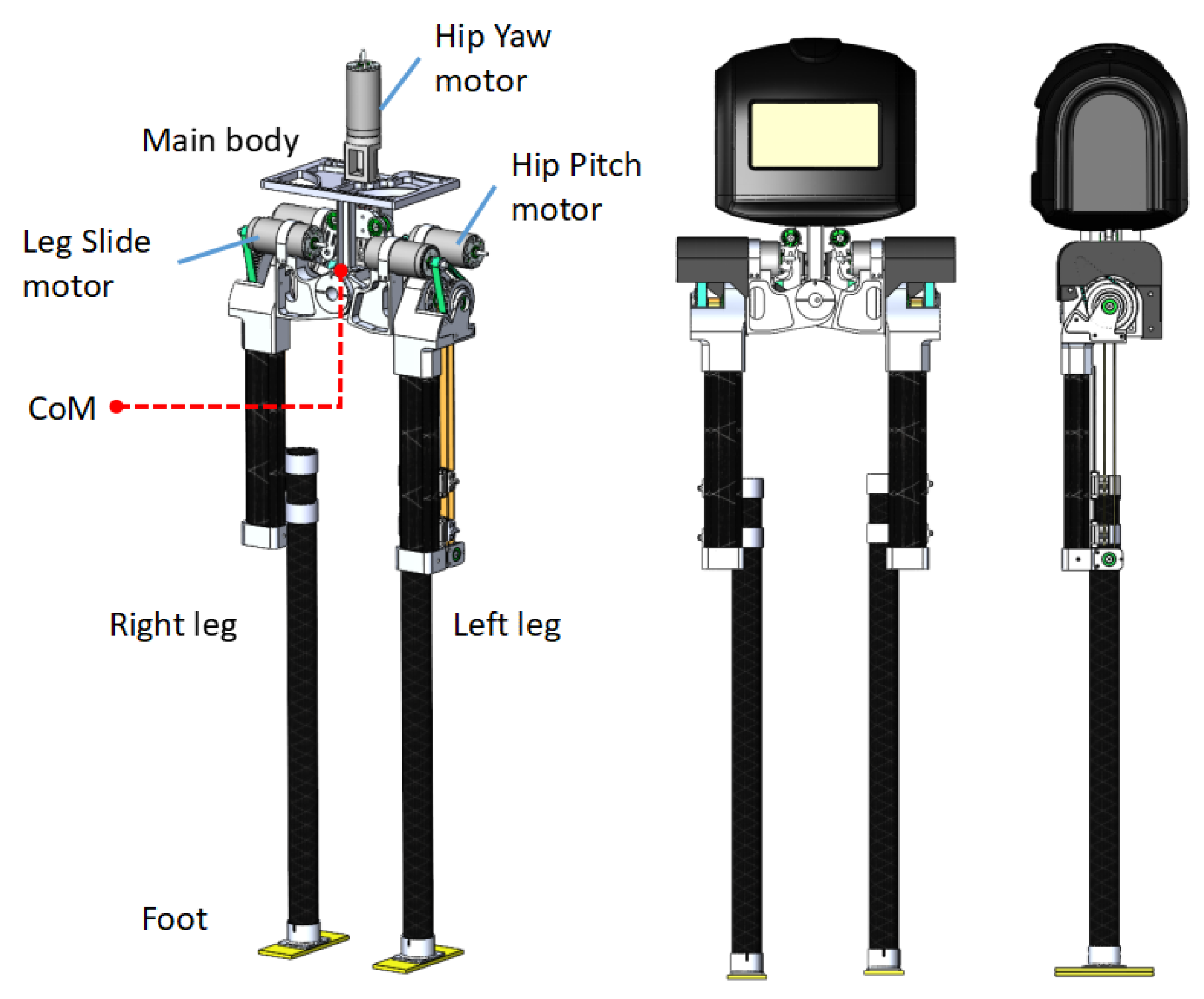
2. Design Overview
2.1. Hip Structure Design
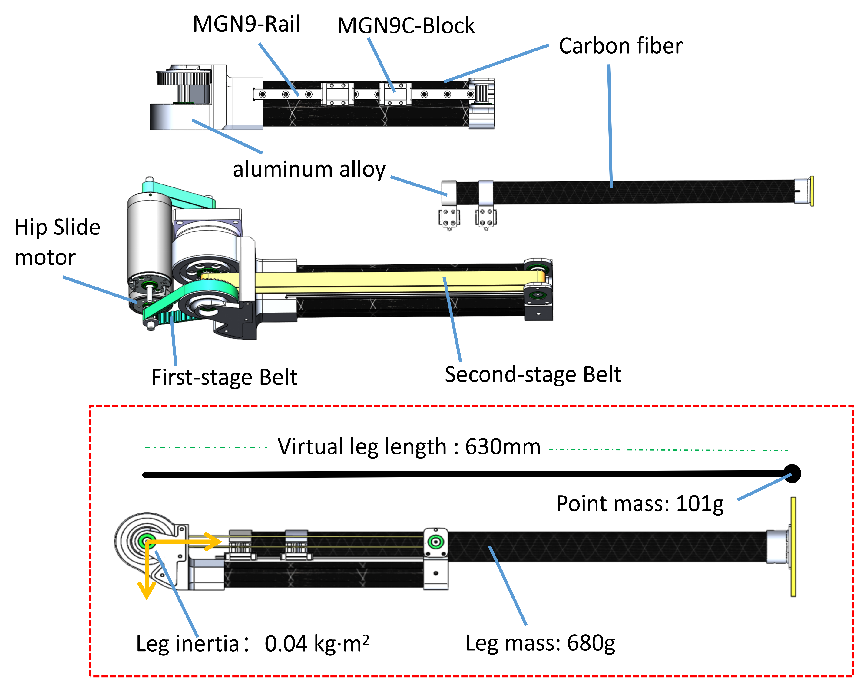
2.2. Leg Structure Design
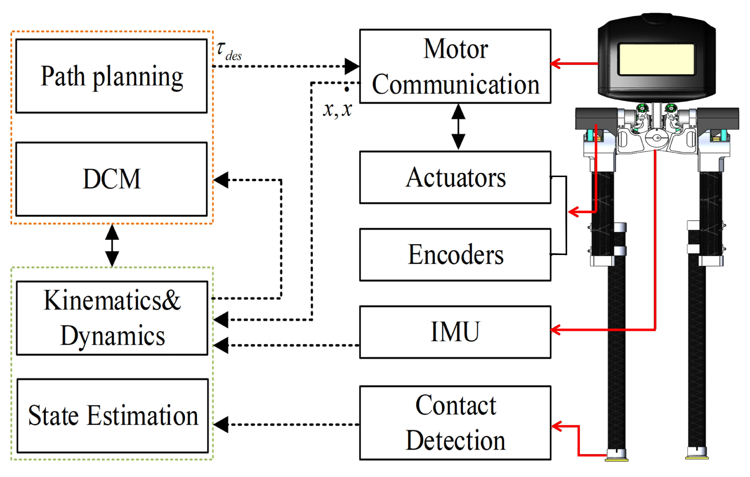
- Due to the unique capabilities of the kneeless telescopic leg design, the robot is able to directly perceive changes in ground contact forces without the need for force sensors, meaning that when the robot’s foot makes contact with the ground, the resulting reaction forces are directly transmitted to the leg motors, enabling the detection of ground contact signals by monitoring changes in electrical currents;
- The dynamic model closely aligns with a simplified mathematical model, and leg telescoping does not introduce anterior–posterior interference;
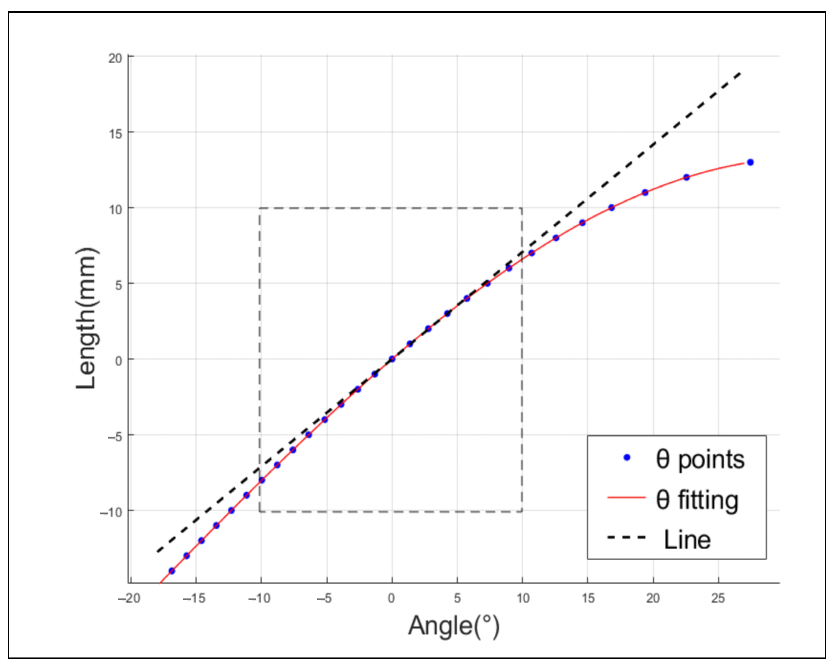
- The kneeless telescoping leg exhibits high linearity;
- Compared to the knee joint approach, the straight leg telescoping joint is more energy-efficient.
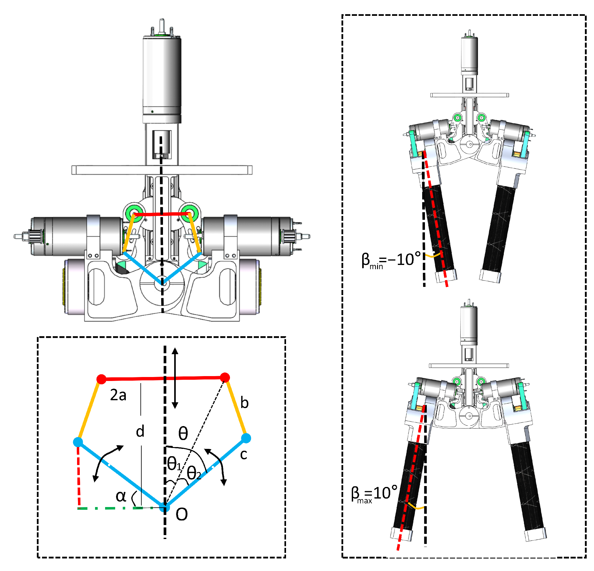
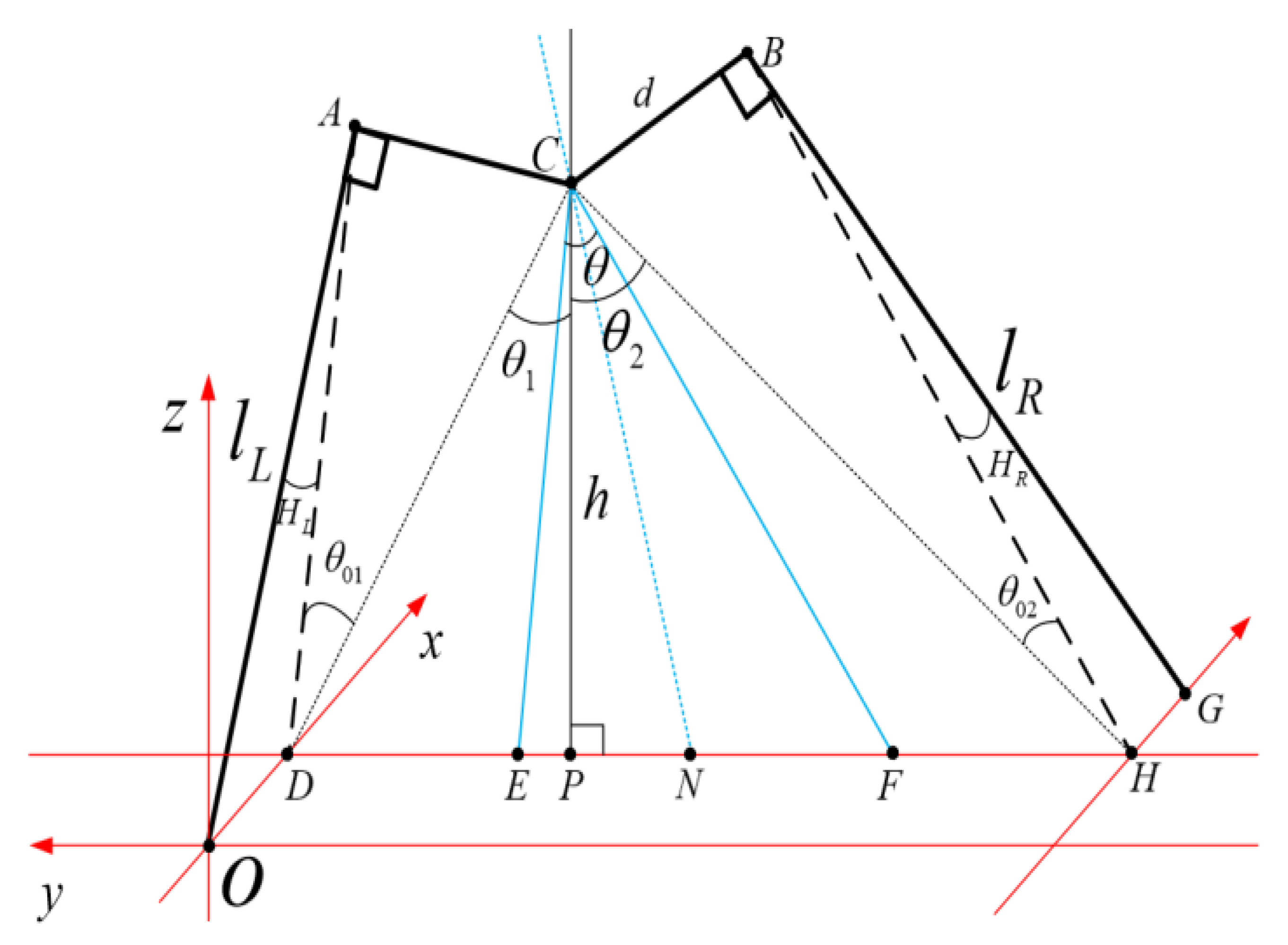
3. Kinematics Analysis
4. Control Principle
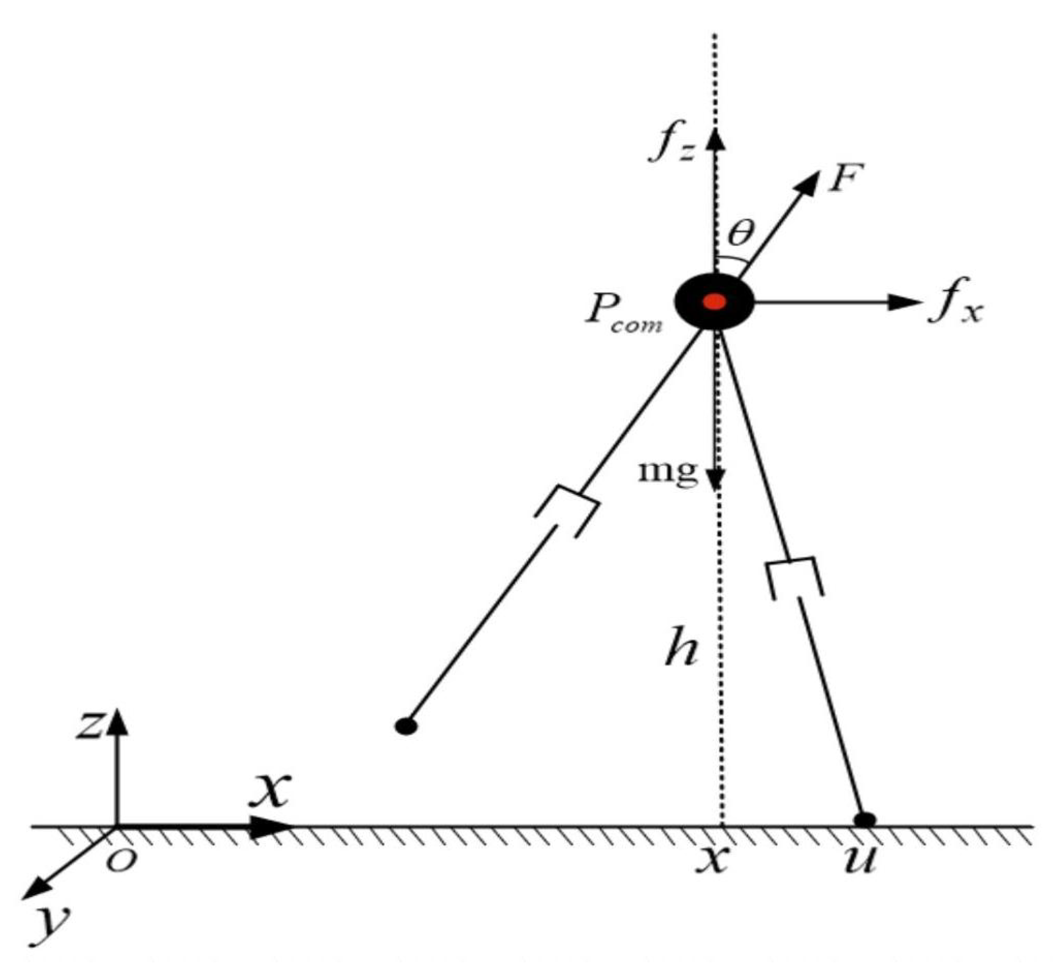
4.1. LIP Dynamics and DCM Derivation
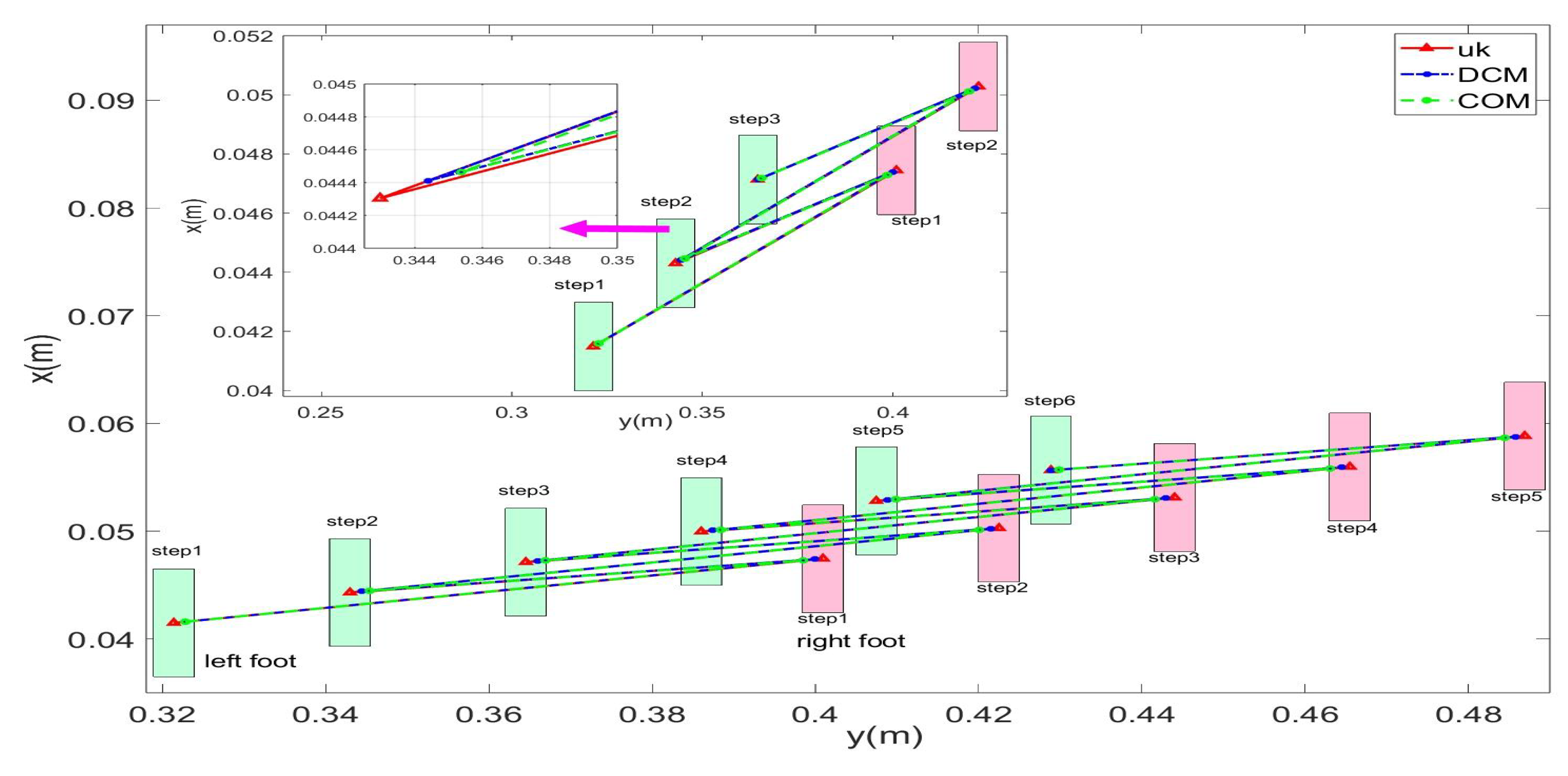
4.2. DCM Trajectory Planning
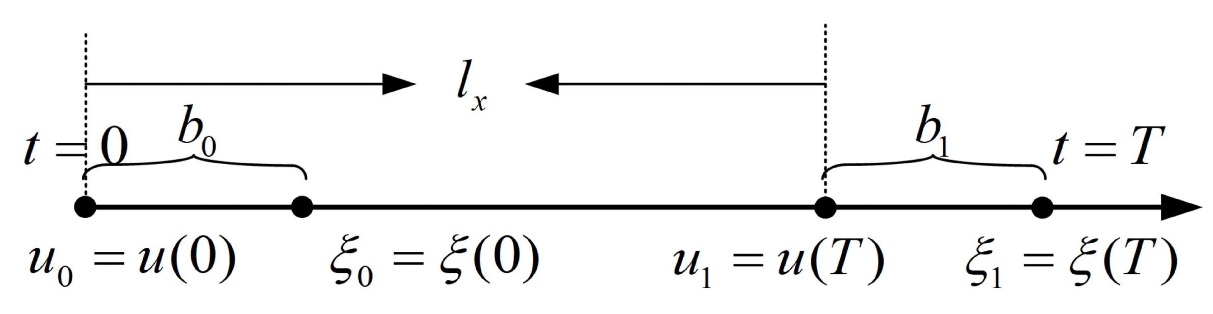
4.2.1. Forward Walking
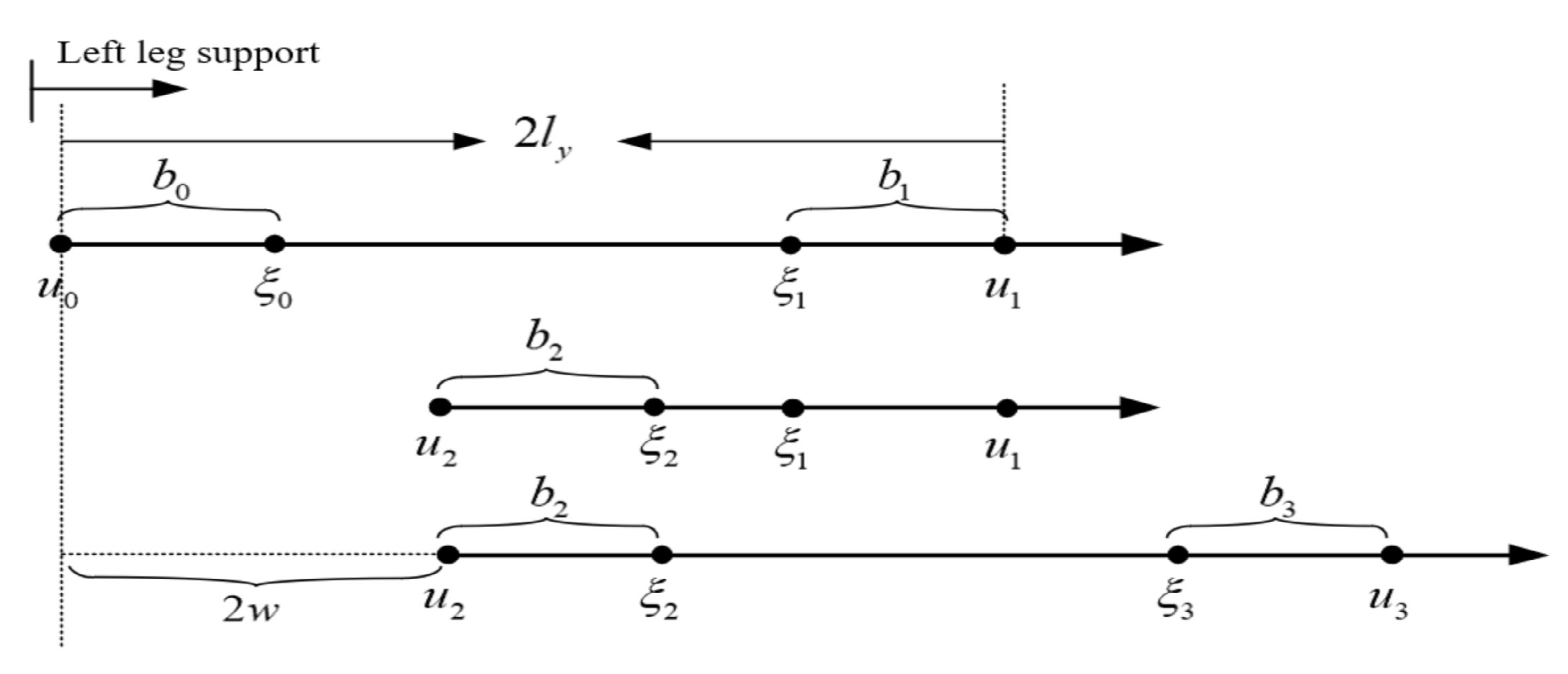
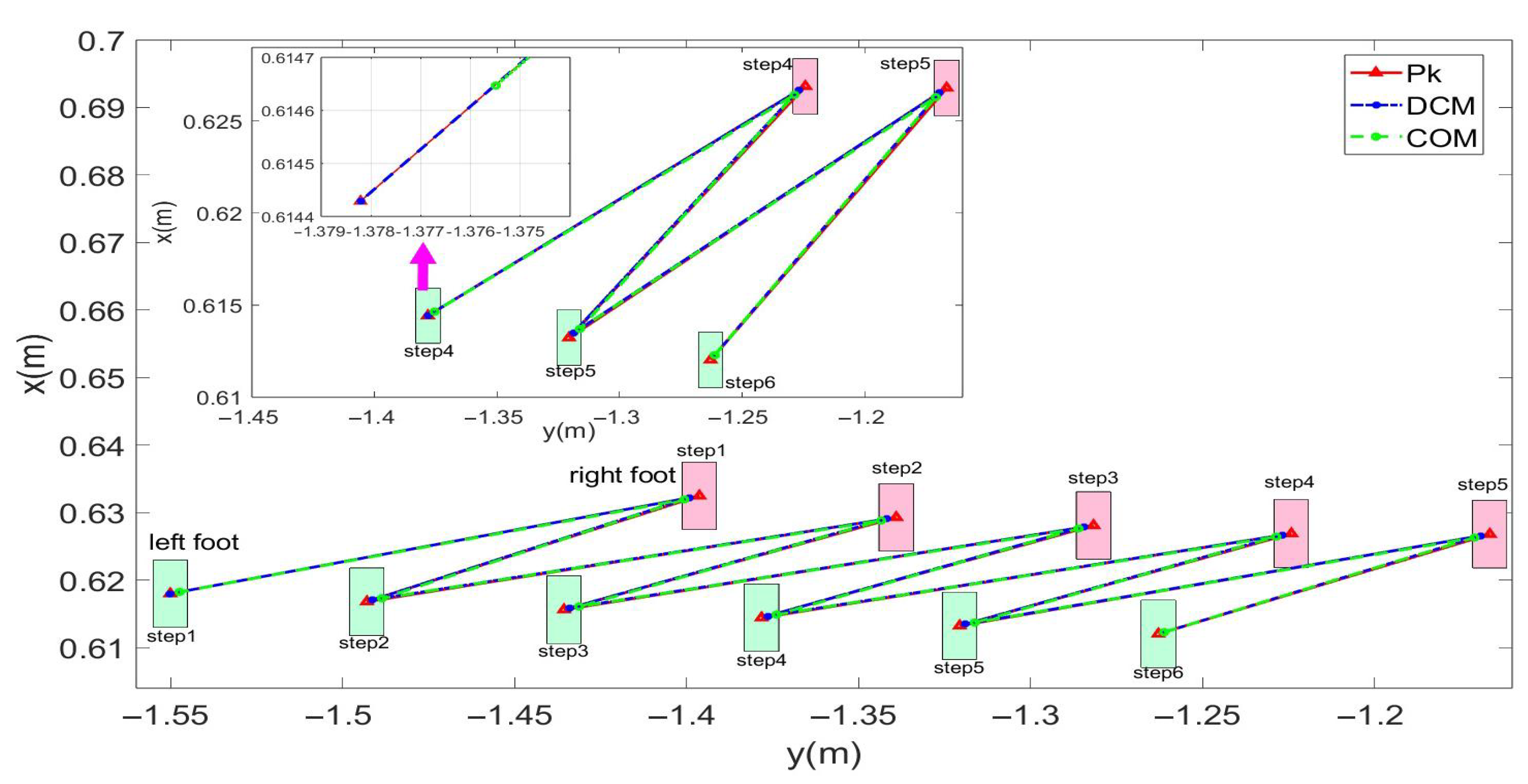
4.2.2. Lateral Walking
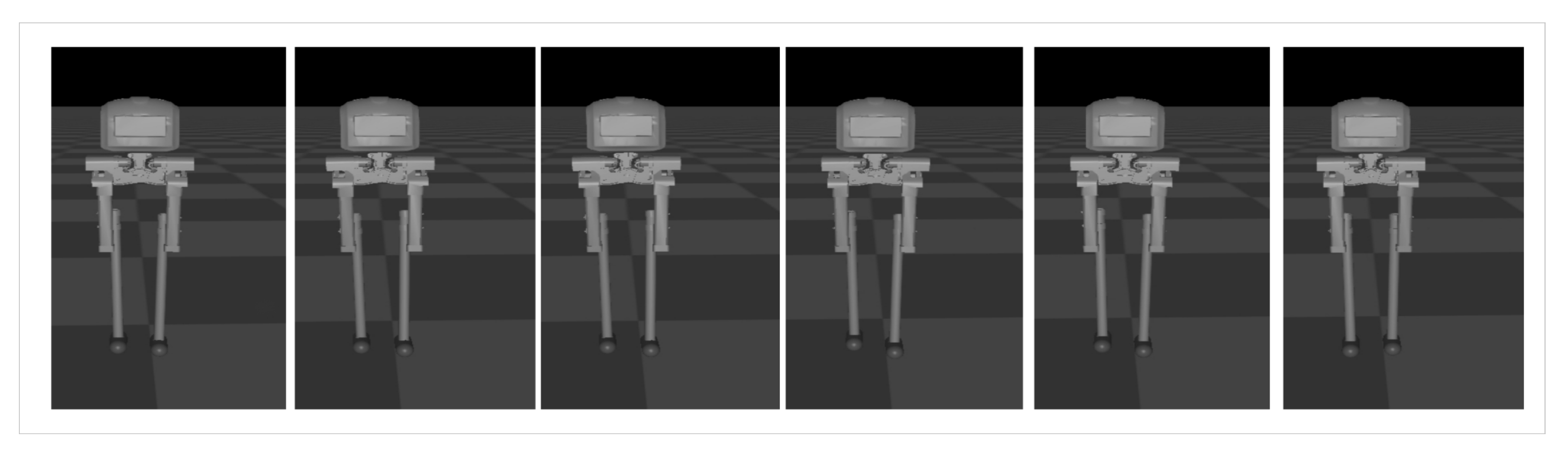
5. Simulations and Experiments
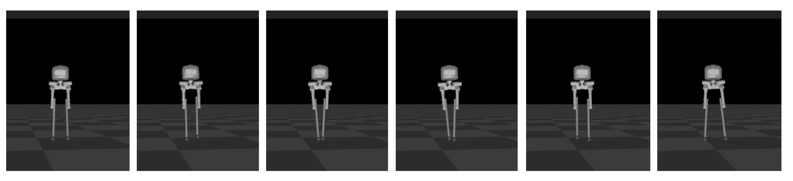
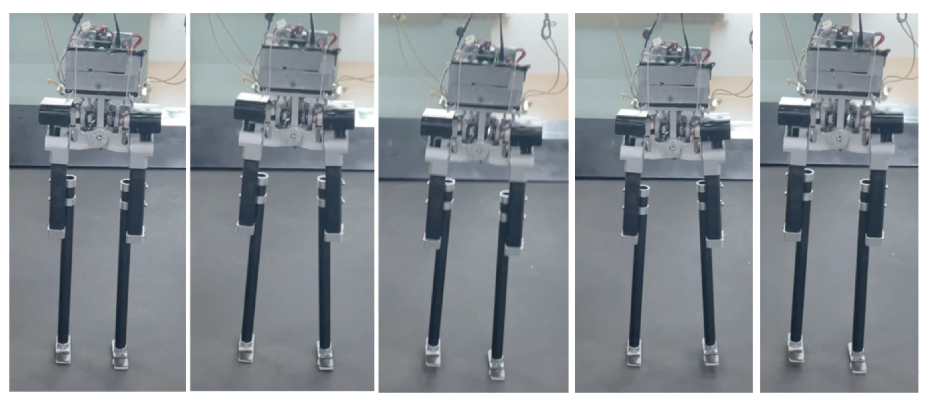
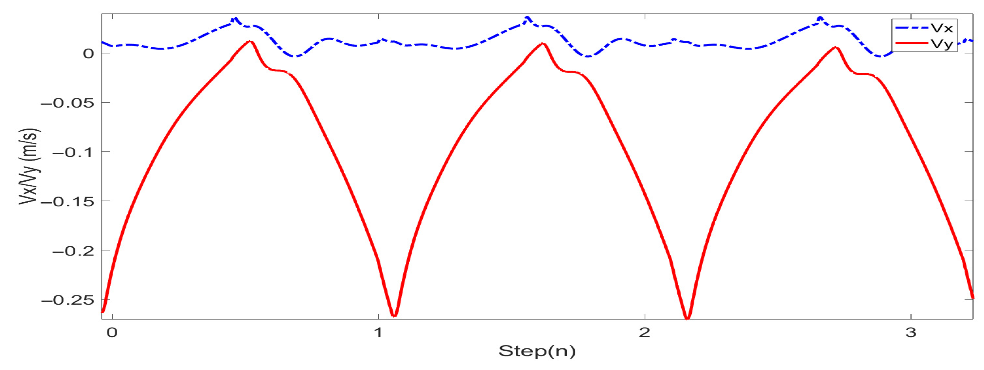
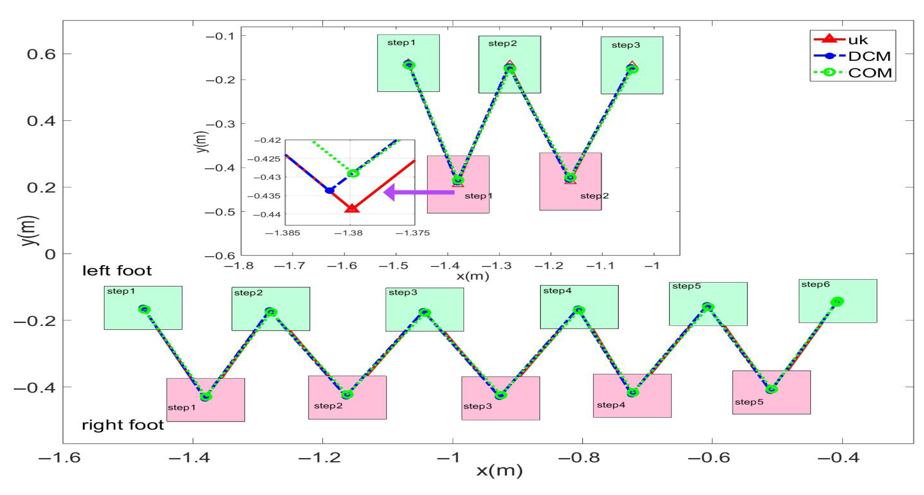
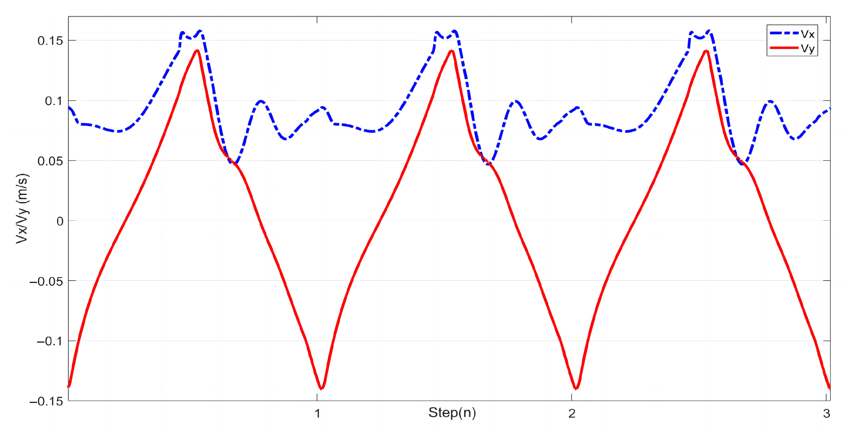
5.1. Sideways Walking
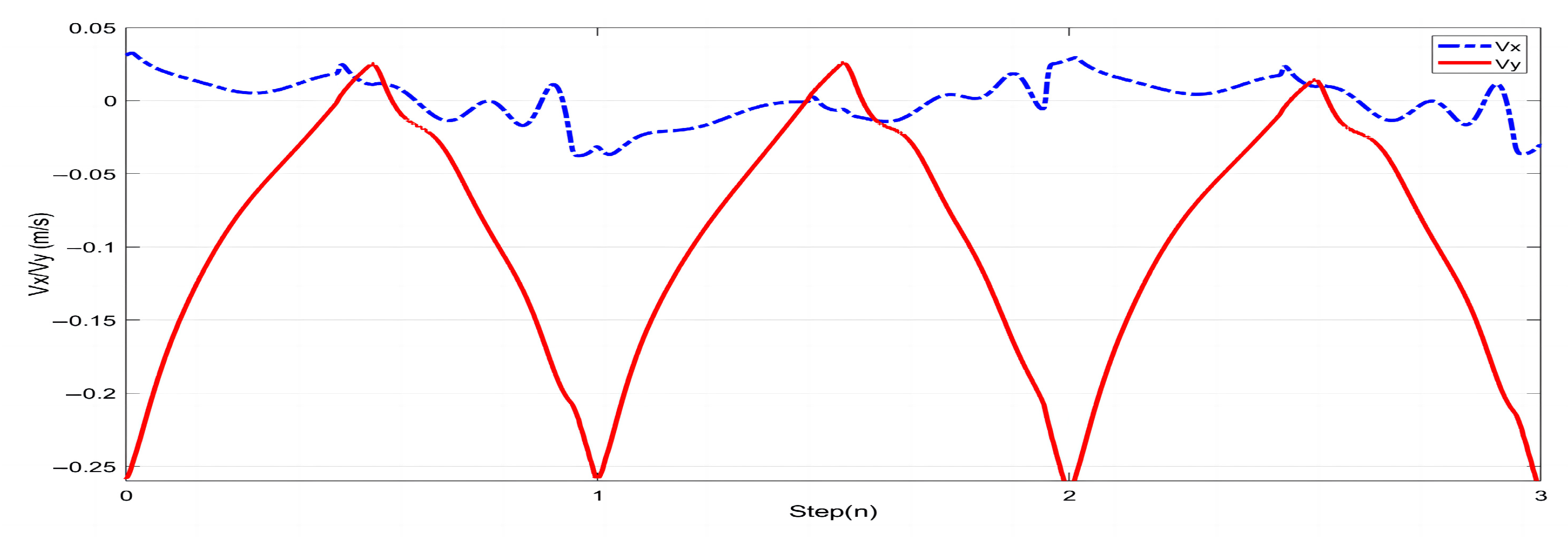
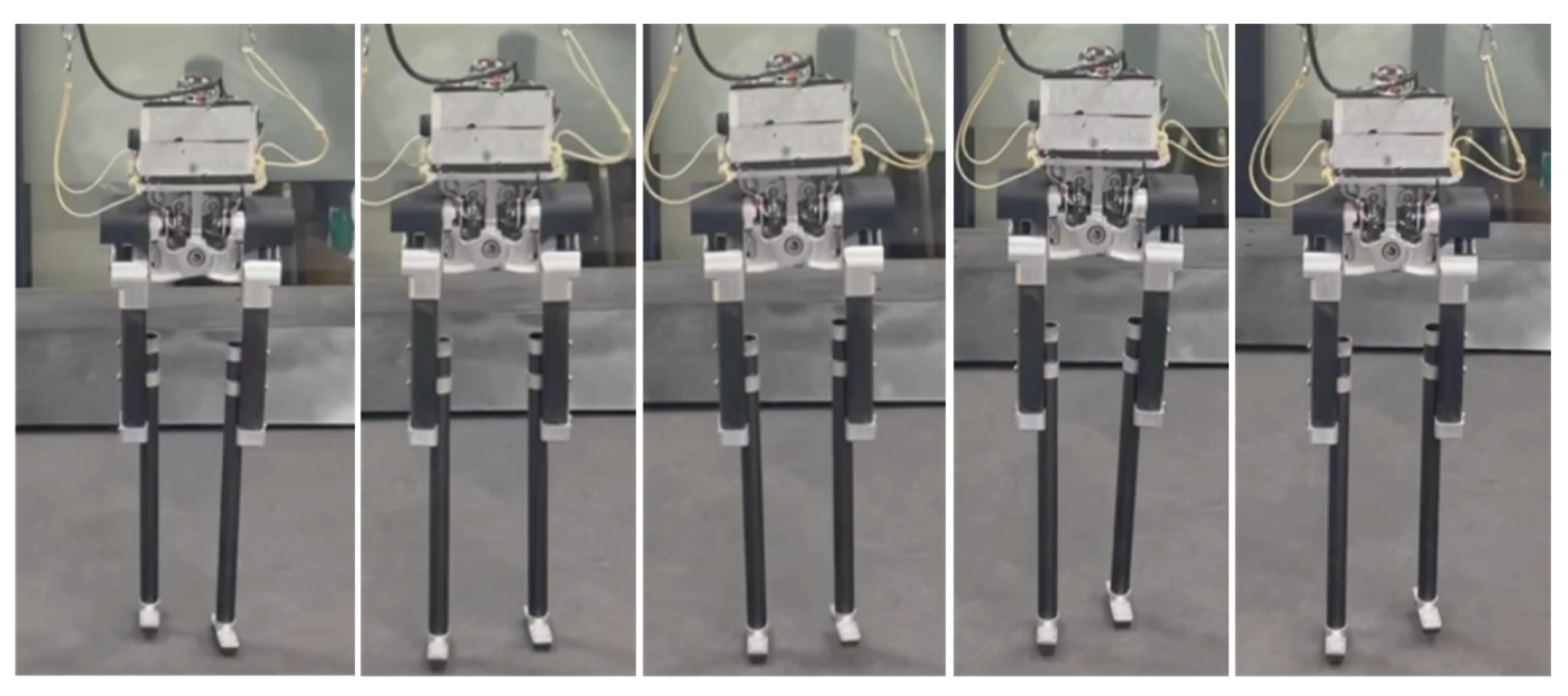
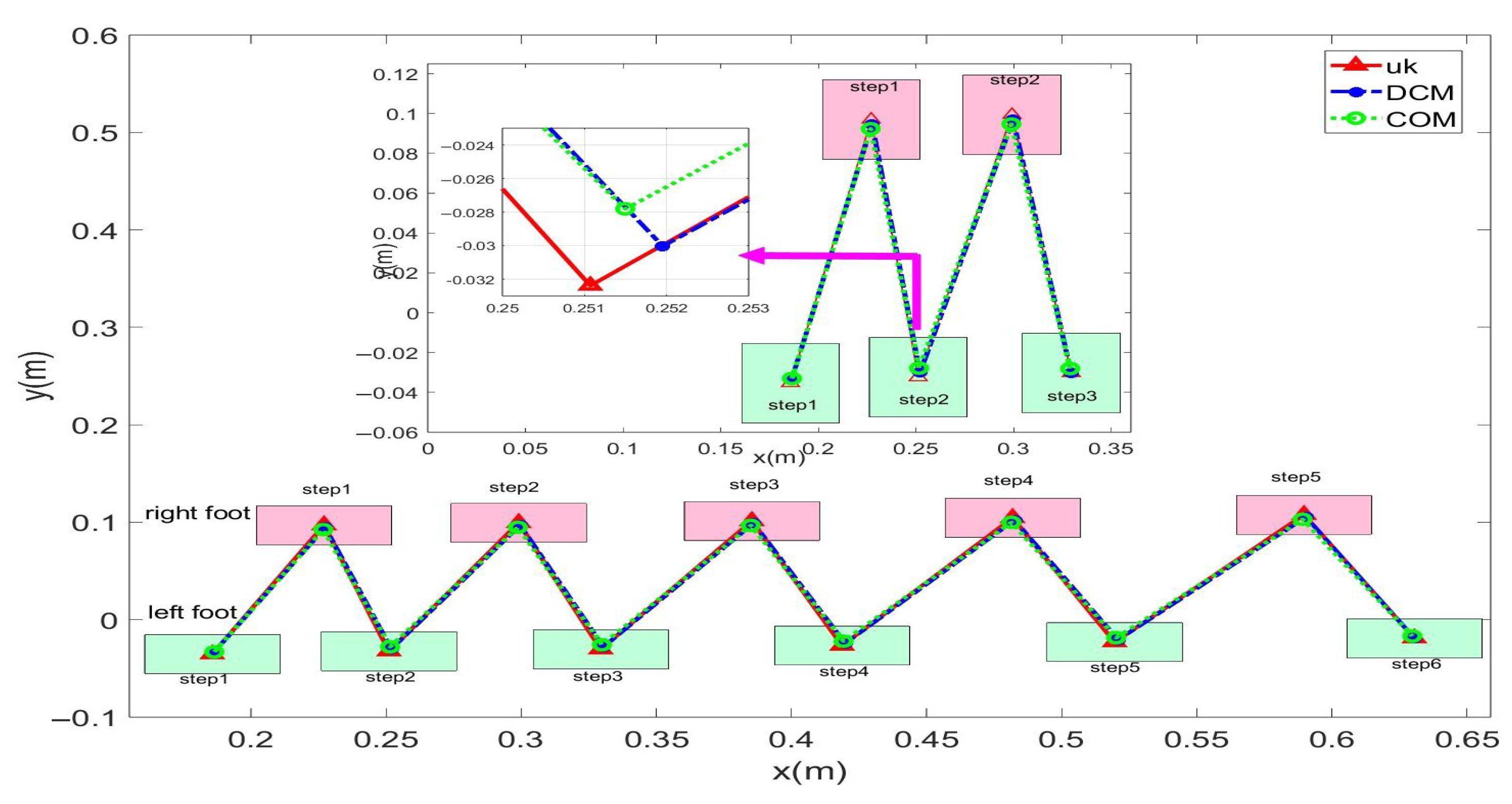
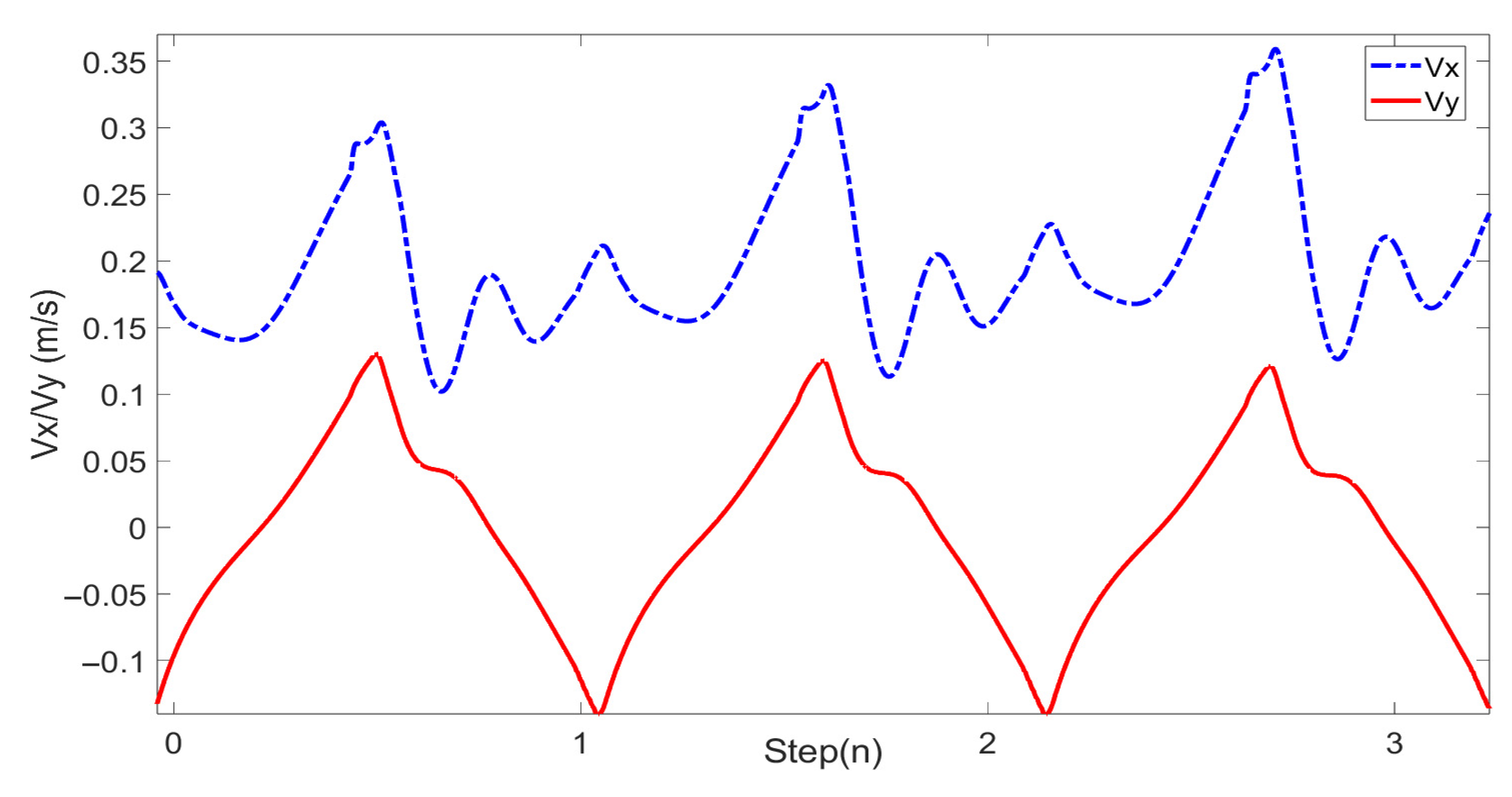
5.2. Forward Walking
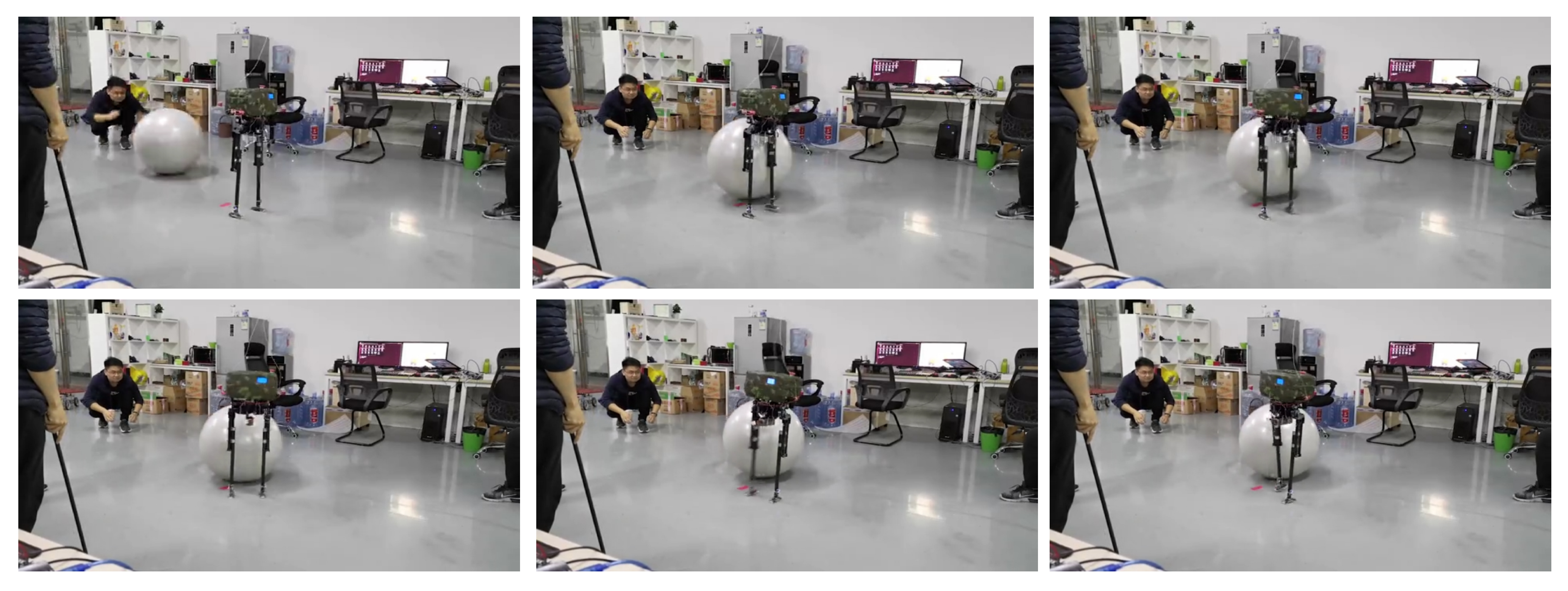
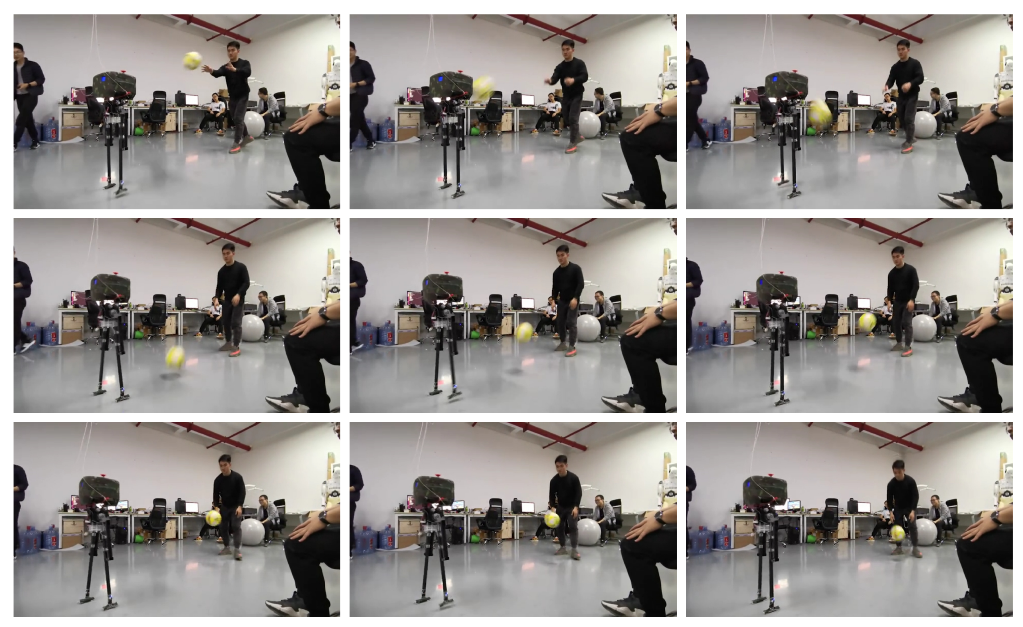
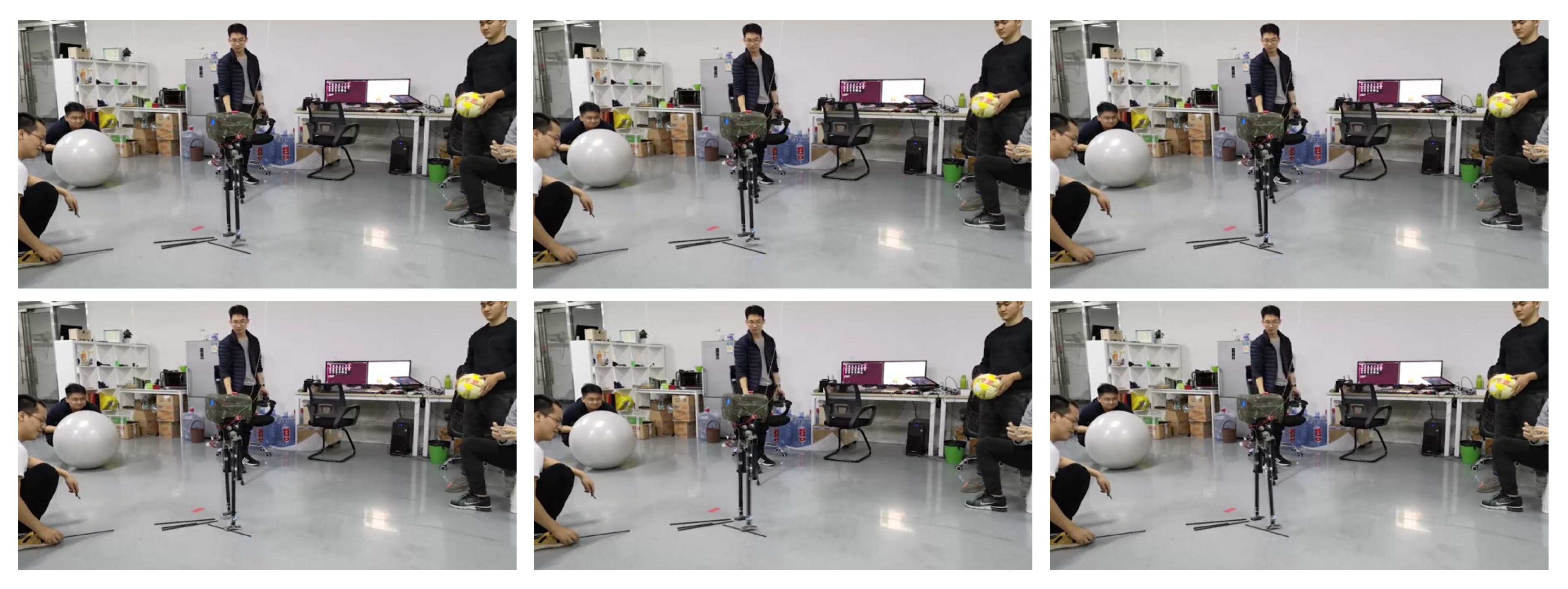
5.3. Stability Analysis
6. Conclusions and Discussion
Author Contributions
Funding
Institutional Review Board Statement
Data Availability Statement
Conflicts of Interest
References
- Farid, Y.; Siciliano, B.; Ruggiero, F. Review and descriptive investigation of the connection between bipedal locomotion and non-prehensile manipulation. Annu. Rev. Control 2022, 53, 51–69. [Google Scholar] [CrossRef]
- Kawato, M.; Europe, I. Humanoid robotics—History, current state of the art, and challenges. Sci. Robot. 2017, 2, eaar4043. [Google Scholar]
- Boston Dynamics: Atlas. Available online: https://www.bostondynamics.com/atlas (accessed on 4 April 2023).
- Chen, J.; Tang, A.; Zhou, G.; Lin, L.; Jiang, G. Walking dynamics for an ascending stair biped robot with telescopic legs and impulse thrust. Electron. Res. Arch. 2022, 30, 4108–4135. [Google Scholar] [CrossRef]
- Meng, M.Q.H.; Song, R. Legged mobile robots for challenging terrains. Biomim. Intell. Robot. 2022, 2, 100034. [Google Scholar] [CrossRef]
- Zhou, G.; Hui, X.; Chen, J.; Jiang, G. Walking dynamics of a semi-passive compass-like robot with impulse thrust. Nonlinear Dyn. 2023, 111, 3307–3325. [Google Scholar] [CrossRef]
- Added, E.; Gritli, H.; Belghith, S. Further analysis of the passive dynamics of the compass biped walker and control of chaos via two trajectory tracking approaches. Complexity 2021, 2021, 5533451. [Google Scholar] [CrossRef]
- Added, E.; Gritli, H.; Belghith, S. Trajectory tracking-based control of the chaotic behavior in the passive bipedal compass-type robot. Eur. Phys. J. Spec. Top. 2022, 231, 1071–1084. [Google Scholar] [CrossRef]
- Chevallereau, C.; Bessonnet, G.; Abba, G.; Aoustin, Y. Bipedal Robots: Modeling, Design and Walking Synthesis; John Wiley & Sons: Hoboken, NJ, USA, 2009. [Google Scholar]
- Aldrich, J.B. Feedback Control of Dynamic Bipedal Robot Locomotion. IEEE Trans. Autom. Control 2008, 53, 1570–1572. [Google Scholar] [CrossRef]
- Gong, Y.; Hartley, R.; Da, X.; Hereid, A.; Harib, O.; Huang, J.K.; Grizzle, J. Feedback control of a cassie bipedal robot: Walking, standing, and riding a segway. In Proceedings of the American Control Conference, Philadelphia, PA, USA, 10–12 July 2019; pp. 4559–4566. [Google Scholar] [CrossRef] [Green Version]
- Daneshmand, E.; Khadiv, M.; Grimminger, F.; Righetti, L. Variable Horizon MPC with Swing Foot Dynamics for Bipedal Walking Control. IEEE Robot. Autom. Lett. 2021, 6, 2349–2356. [Google Scholar] [CrossRef]
- Wang, K.; Marsh, D.; Saputra, R.P.; Chappell, D.; Jiang, Z.; Raut, A.; Kon, B.; Kormushev, P. Design and Control of SLIDER: An Ultra-lightweight, Knee-less, Low-cost Bipedal Walking Robot. In Proceedings of the 2020 IEEE/RSJ International Conference on Intelligent Robots and Systems (IROS), Las Vegas, NV, USA, 25–29 October 2020; pp. 3488–3495. [Google Scholar]
- Bhounsule, P.A.; Cortell, J.; Ruina, A. Design and control of ranger: An energy-efficient, dynamic walking robot. Adapt. Mob. Robot. 2012, 441–448. [Google Scholar] [CrossRef] [Green Version]
- Li, Q.; Liu, G.; Tang, J.; Zhang, J. A simple 2D straight-leg passive dynamic walking model without foot-scuffing problem. In Proceedings of the IEEE International Conference on Intelligent Robots and Systems, Daejeon, South Korea, 9–14 October 2016; pp. 5155–5161. [Google Scholar] [CrossRef]
- Hashimoto, K. Mechanics of humanoid robot. Adv. Robot. 2020, 34, 1390–1397. [Google Scholar] [CrossRef]
- Lohmeier, S. Design and Realization of a Humanoid Robot for Fast and Autonomous Bipedal Locomotion. Ph.D. Thesis, Technische Universität München, Munich, Germany, 2010. [Google Scholar]
- Harata, Y.; Kato, Y.; Asano, F. Efficiency analysis of telescopic-legged bipedal robots. Artif. Life Robot. 2018, 23, 585–592. [Google Scholar] [CrossRef]
- Roig, A.; Kishor Kothakota, S.; Miguel, N.; Fernbach, P.; Hoffman, E.M.; Marchionni, L. On the Hardware Design and Control Architecture of the Humanoid Robot Kangaroo. In Proceedings of the 6th Workshop on Legged Robots during the International Conference on Robotics and Automation (ICRA 2022), Philadelphia, PA, USA, 27 May 2022. [Google Scholar]
- Causeim. Available online: https://sites.google.com/view/causeim/home (accessed on 4 April 2023).
- Buss, B.G.; Hamed, K.A.; Griffin, B.A.; Grizzle, J.W. Experimental results for 3D bipedal robot walking based on systematic optimization of virtual constraints. In Proceedings of the American Control Conference, Boston, MA, USA, 6–8 July 2016; pp. 4785–4792. [Google Scholar] [CrossRef]
- Abate, A.; Hatton, R.L.; Hurst, J. Passive-dynamic leg design for agile robots. In Proceedings of the IEEE International Conference on Robotics and Automation, Seattle, WA, USA, 26–30 May 2015; pp. 4519–4524. [Google Scholar] [CrossRef]
- Hubicki, C.; Grimes, J.; Jones, M.; Renjewski, D.; Spröwitz, A.; Abate, A.; Hurst, J. ATRIAS: Design and validation of a tether-free 3D-capable spring-mass bipedal robot. Int. J. Robot. Res. 2016, 35, 1497–1521. [Google Scholar] [CrossRef]
- Kajita, S.; Kanehiro, F.; Kaneko, K.; Fujiwara, K.; Harada, K.; Yokoi, K.; Hirukawa, H. Biped walking pattern generation by using preview control of zero-moment point. Proc.-IEEE Int. Conf. Robot. Autom. 2003, 2, 1620–1626. [Google Scholar] [CrossRef] [Green Version]
- Kamioka, T.; Kaneko, H.; Takenaka, T.; Yoshiike, T. Simultaneous Optimization of ZMP and Footsteps Based on the Analytical Solution of Divergent Component of Motion. In Proceedings of the IEEE International Conference on Robotics and Automation, Brisbane, QLD, Australia, 21–25 May 2018; pp. 1763–1770. [Google Scholar] [CrossRef]
- Schuller, R.; Mesesan, G.; Englsberger, J.; Lee, J.; Ott, C. Online Learning of Centroidal Angular Momentum towards Enhancing DCM-based Locomotion. In Proceedings of the IEEE International Conference on Robotics and Automation, Philadelphia, PA, USA, 23–27 May 2022; pp. 10442–10448. [Google Scholar] [CrossRef]
- Wang, K.; Xin, G.; Xin, S.; Mistry, M.; Vijayakumar, S.; Kormushev, P. A Unified Model with Inertia Shaping for Highly Dynamic Jumps of Legged Robots. arXiv 2021, arXiv:2109.04581. [Google Scholar]
- Zhang, Z.; Zhang, L.; Xin, S.; Xiao, N.; Wen, X. Robust Walking for Humanoid Robot Based on Divergent Component of Motion. Micromachines 2022, 13, 1095. [Google Scholar] [CrossRef]


| Parameter | Quantitative Value | |
|---|---|---|
| length | / | 0.284 m |
| width | / | 0.16 m |
| height | normal | 0.92 m |
| highest | 0.94 m | |
| lowest | 0.84 m | |
| weight | total | 5.5 kg |
| hip | 4.41 kg | |
| leg | 0.68 kg | |
| lateral hip | range | −10° to 10° |
| peak velocity | 155°/s | |
| peak torque | 195 Nm | |
| pitch hip | range | −90° to 90° |
| peak velocity | 540°/s | |
| peak torque | 56 Nm | |
| slide leg | leg length range | 580 mm to 680 mm |
| peak velocity | 1.5 m/s | |
| peak force | 1120 N | |
Disclaimer/Publisher’s Note: The statements, opinions and data contained in all publications are solely those of the individual author(s) and contributor(s) and not of MDPI and/or the editor(s). MDPI and/or the editor(s) disclaim responsibility for any injury to people or property resulting from any ideas, methods, instructions or products referred to in the content. |
© 2023 by the authors. Licensee MDPI, Basel, Switzerland. This article is an open access article distributed under the terms and conditions of the Creative Commons Attribution (CC BY) license (https://creativecommons.org/licenses/by/4.0/).
Share and Cite
Tang, J.; Zhu, Y.; Gan, W.; Mou, H.; Leng, J.; Li, Q.; Yu, Z.; Zhang, J. Design, Control, and Validation of a Symmetrical Hip and Straight-Legged Vertically-Compliant Bipedal Robot. Biomimetics 2023, 8, 340. https://doi.org/10.3390/biomimetics8040340
Tang J, Zhu Y, Gan W, Mou H, Leng J, Li Q, Yu Z, Zhang J. Design, Control, and Validation of a Symmetrical Hip and Straight-Legged Vertically-Compliant Bipedal Robot. Biomimetics. 2023; 8(4):340. https://doi.org/10.3390/biomimetics8040340
Chicago/Turabian StyleTang, Jun, Yudi Zhu, Wencong Gan, Haiming Mou, Jie Leng, Qingdu Li, Zhiqiang Yu, and Jianwei Zhang. 2023. "Design, Control, and Validation of a Symmetrical Hip and Straight-Legged Vertically-Compliant Bipedal Robot" Biomimetics 8, no. 4: 340. https://doi.org/10.3390/biomimetics8040340