
Opponent Hitting Behavior Prediction and Ball Location Control for a Table Tennis Robot

Abstract
:1. Introduction
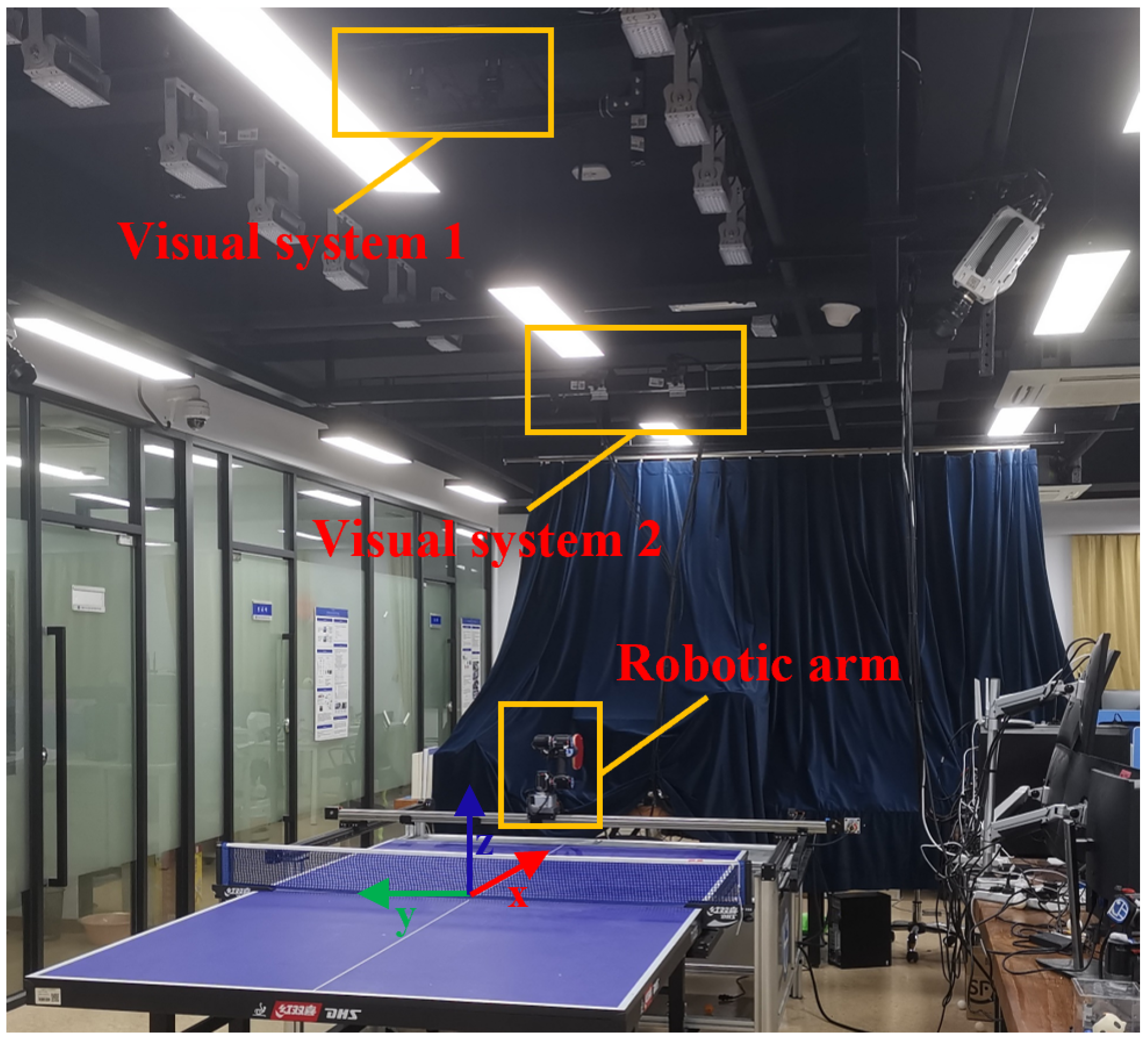
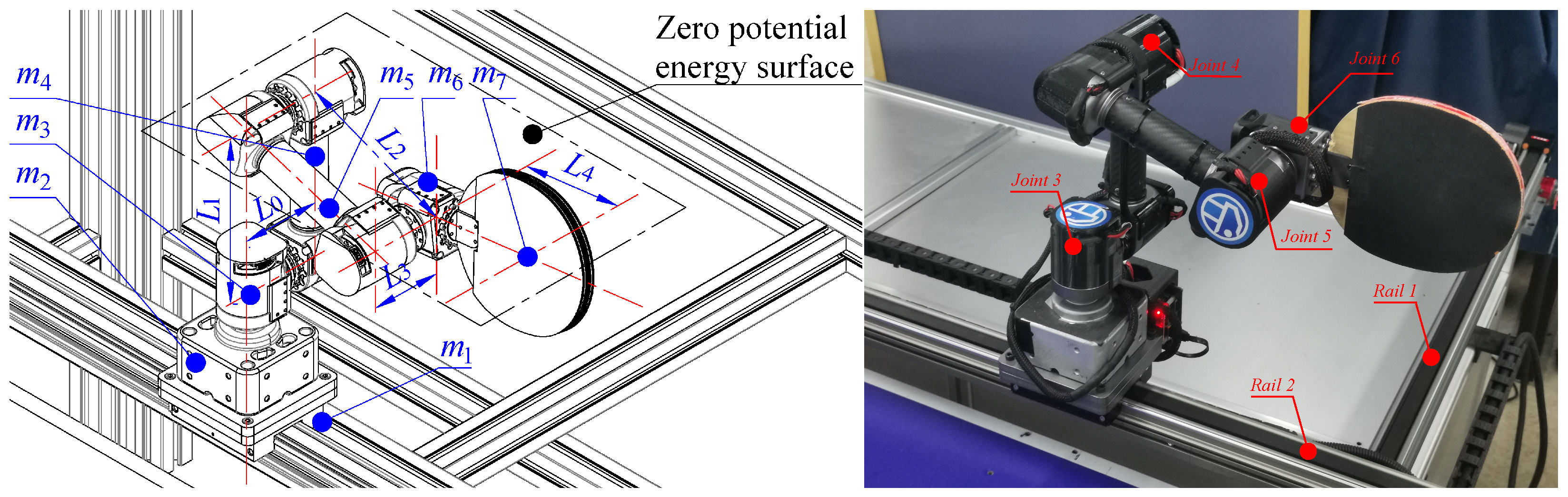
2. The Table Tennis Robot System
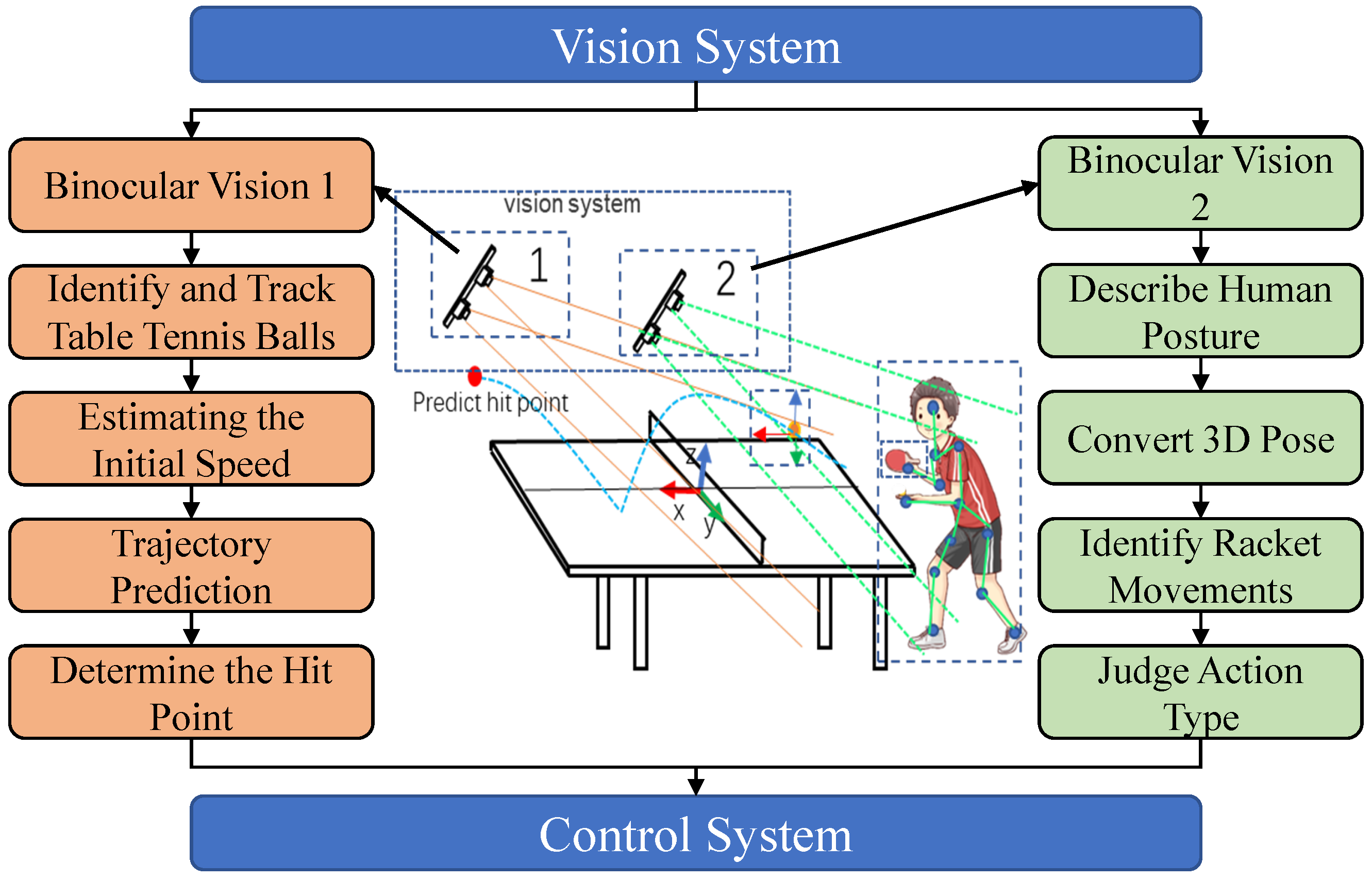
3. The Vision Module
3.1. Trajectory Prediction of Balls
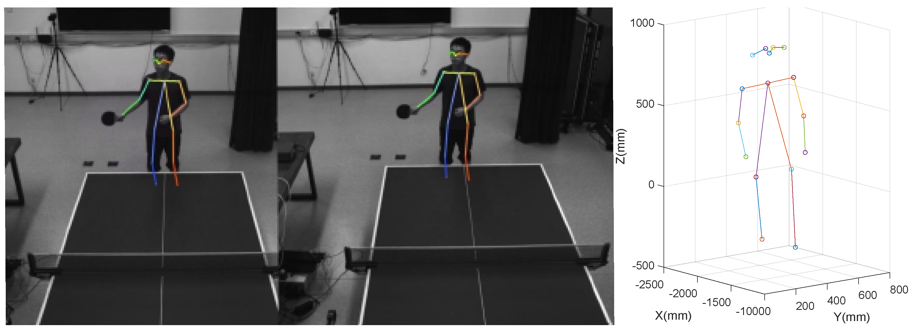
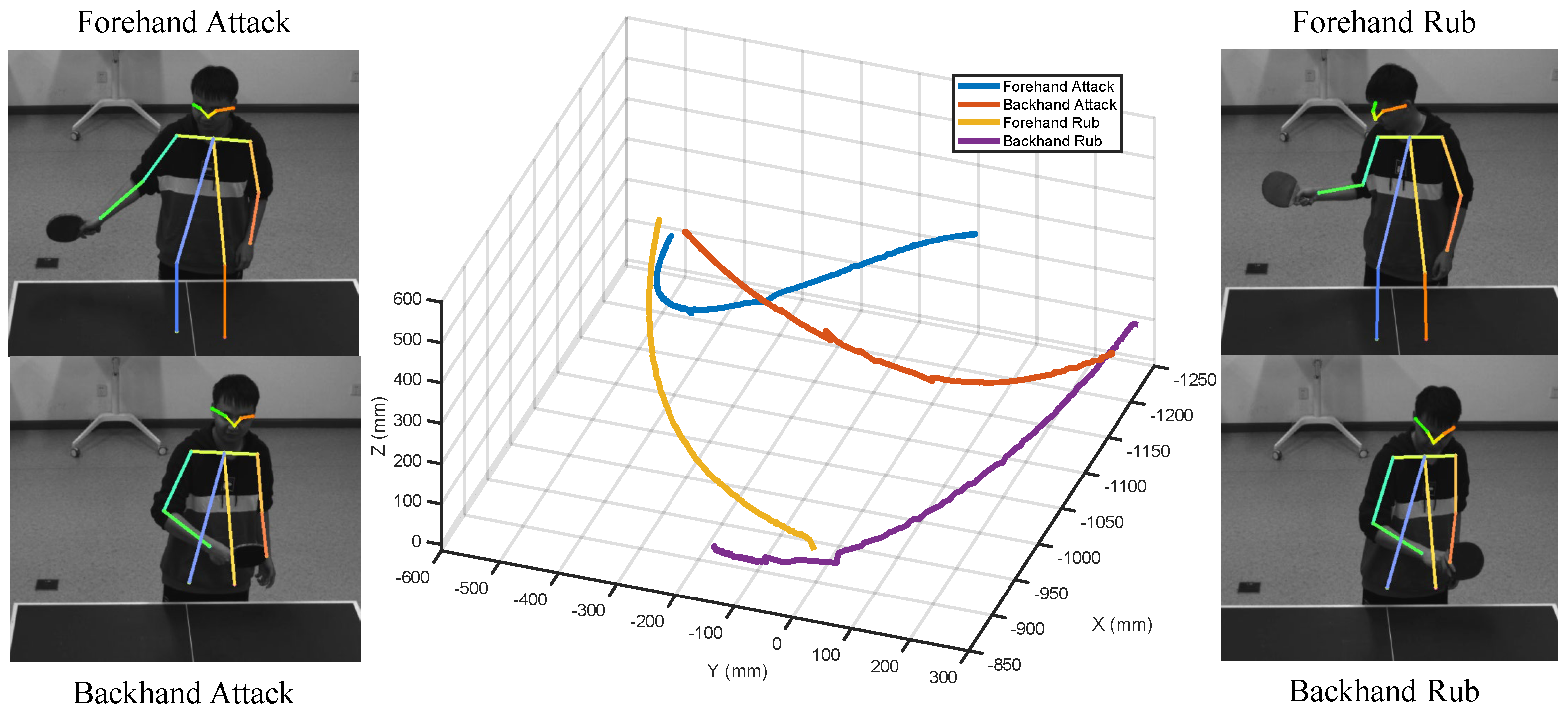
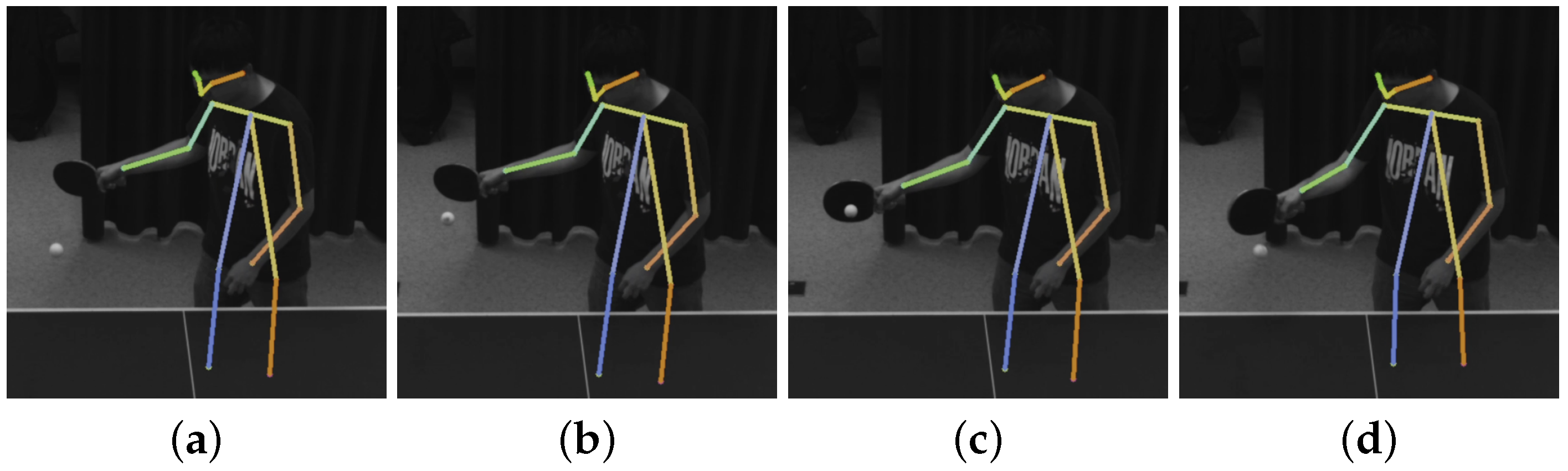
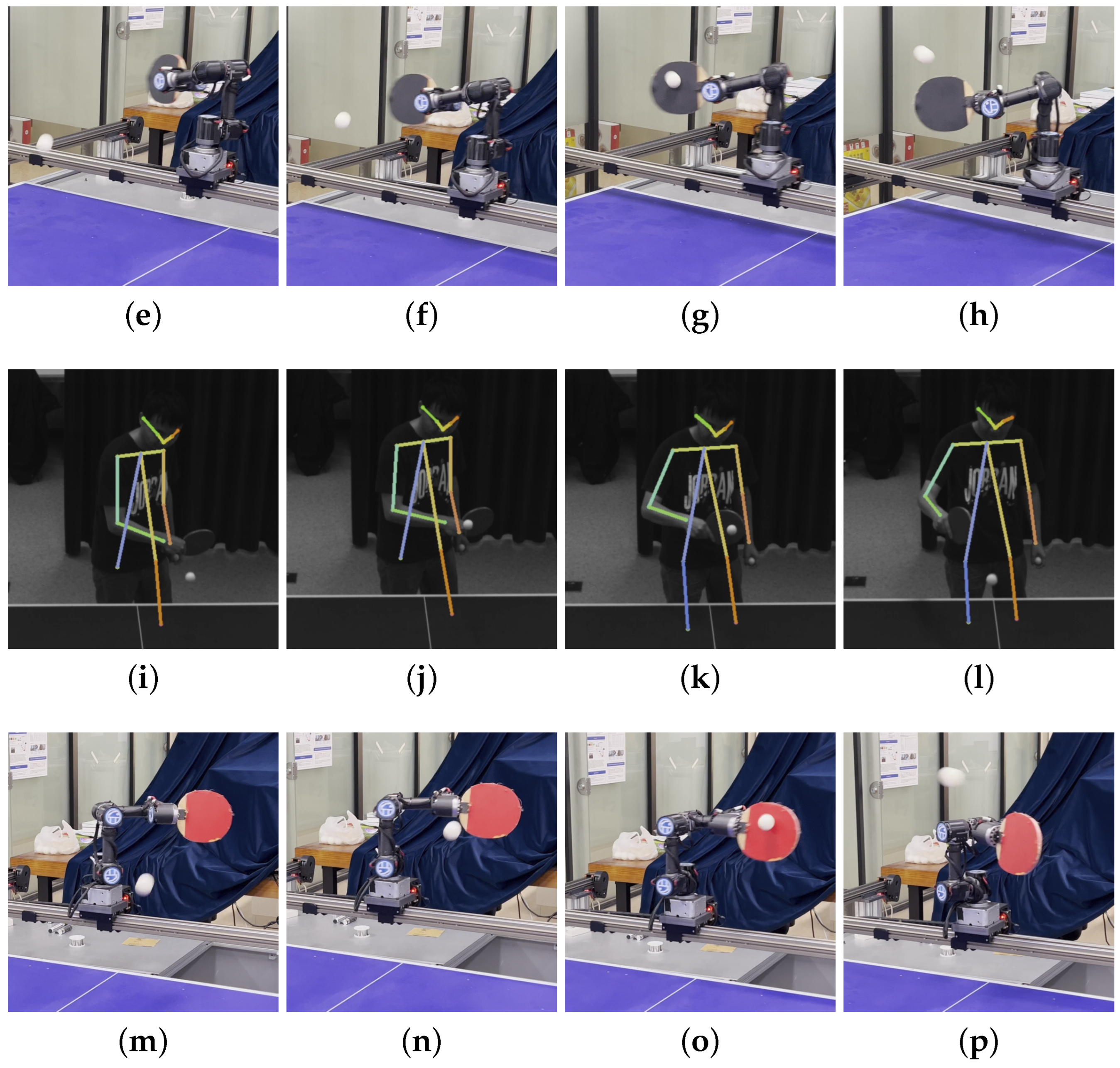
3.2. Stroke Type Classification and Rotation Type Prediction
4. Humanoid Robotic Arm Control
4.1. Joint Position Calculation
| Algorithm 1: Solving parameters of |
Solving Solving Solving Solving or
Solving Solving Solving |
4.2. Joint Velocity Calculation and Trajectory Planning
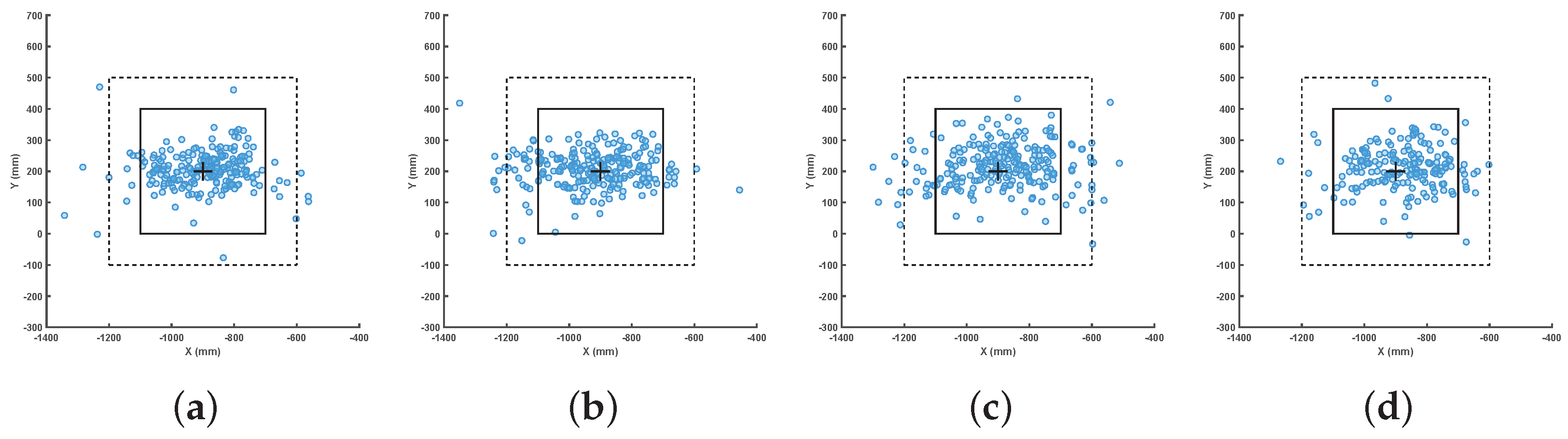
5. Ball Location Control
| Algorithm 2: Solutions of the nonlinear equations |
Step 1: Let Equation (14) be , Equation (15) be , and Equation (16) be . Let , , if , and if . Let the jacobian matrix be
Step 2: Solving elements of : , , , , , , , , Step 3: Let . Step 4: Calculate . Step 5: If , return , and otherwise, set and go to Step 4. |
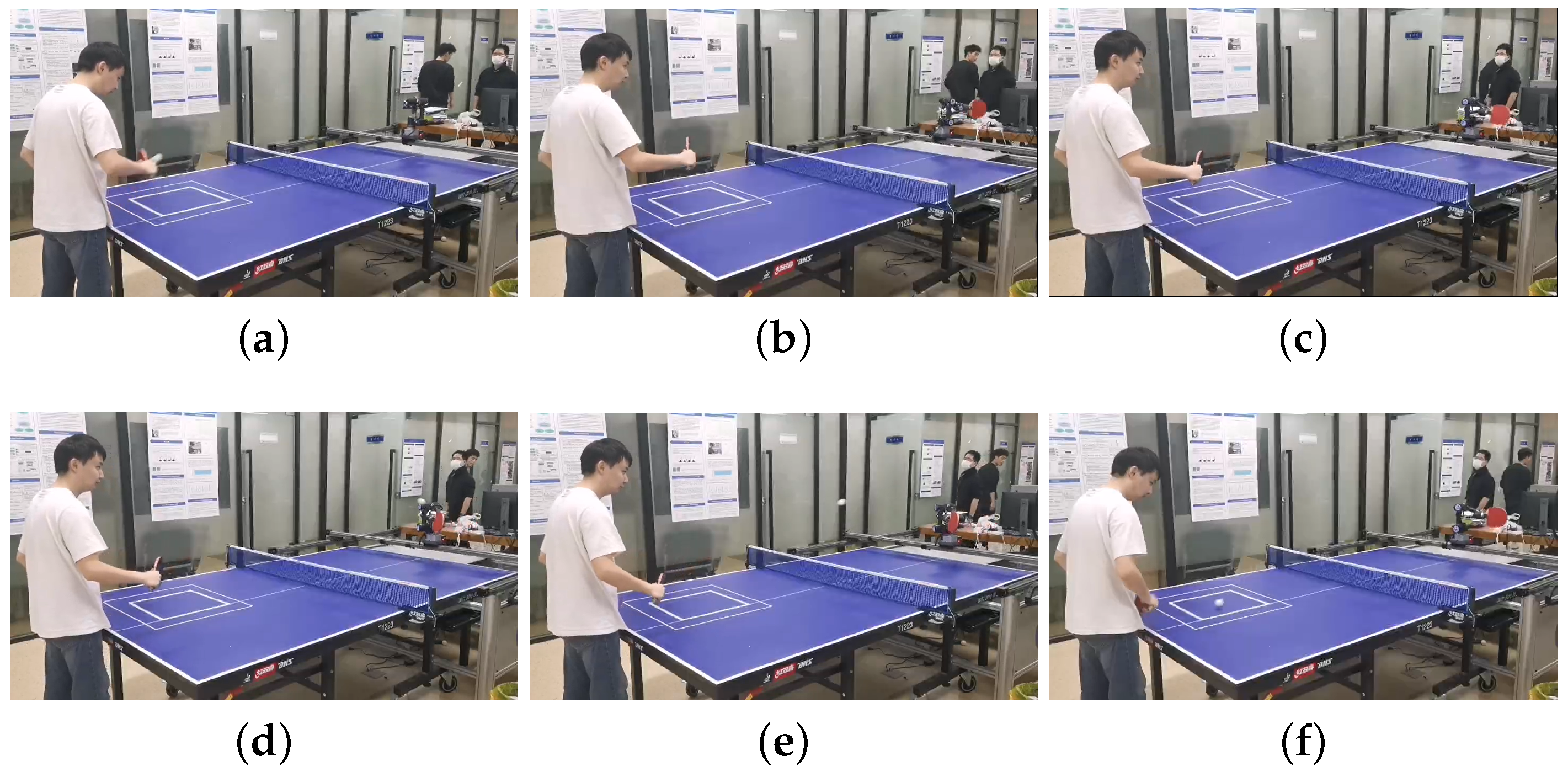
6. Experiment
7. Conclusions
Author Contributions
Funding
Institutional Review Board Statement
Informed Consent Statement
Data Availability Statement
Conflicts of Interest
References
- Li, Y.; Li, B.; Ruan, J.; Rong, X. Research of mammal bionic quadruped robots: A review. In Proceedings of the 5th IEEE Conference on Robotics, Automation and Mechatronics (RAM), Qingdao, China, 17–19 September 2011; pp. 166–171. [Google Scholar]
- Fan, X.; Sayers, W.; Zhang, S.; Han, Z.; Chizari, H. Review and Classification of Bio-inspired Algorithms and Their Applications. J. Bionic Eng. 2020, 17, 611–631. [Google Scholar] [CrossRef]
- Mukherjee, D.; Gupta, K.; Li, H.C.; Najjaran, H. A Survey of Robot Learning Strategies for Human-Robot Collaboration in Industrial Settings. Robot. Comput.-Integr. Manuf. 2022, 73, 102231. [Google Scholar] [CrossRef]
- Arents, J.; Greitans, M. Smart industrial robot control trends, challenges and opportunities within manufacturing. Appl. Sci. 2022, 12, 937. [Google Scholar] [CrossRef]
- Billard, A.; Kragic, D. Trends and challenges in robot manipulation. Science 2019, 364, eaat8414. [Google Scholar] [CrossRef] [PubMed]
- Tang, C.; Sun, L.; Zhou, G.; Shu, X.; Tang, H.; Wu, H. Gait Generation Method of Snake Robot Based on Main Characteristic Curve Fitting. Biomimetics 2023, 8, 105. [Google Scholar] [CrossRef] [PubMed]
- Gu, S.; Meng, F.; Liu, B.; Zhang, Z.; Sun, N.; Wang, M. Stability Control of Quadruped Robot Based on Active State Adjustment. Biomimetics 2023, 8, 112. [Google Scholar] [CrossRef] [PubMed]
- Guo, X.; Ma, S.; Li, B.; Fang, Y. A Novel Serpentine Gait Generation Method for Snakelike Robots Based on Geometry Mechanics. IEEE/ASME Trans. Mechatron. 2018, 23, 1249–1258. [Google Scholar] [CrossRef]
- Zhang, Y.; Wu, Z.; Wang, J.; Tan, M. Design and Analysis of a Bionic Gliding Robotic Dolphin. Biomimetics 2023, 8, 151. [Google Scholar] [CrossRef] [PubMed]
- Seok, S.; Wang, A.; Meng, Y.C.; Otten, D.; Lang, J.; Kim, S. Design principles for highly efficient quadrupeds and implementation on the MIT Cheetah robot. In Proceedings of the 2013 IEEE International Conference on Robotics and Automation, Karlsruhe, Germany, 6–10 May 2013. [Google Scholar]
- Liu, G.H.; Lin, H.Y.; Lin, H.Y.; Chen, S.T.; Lin, P.C. A Bio-Inspired Hopping Kangaroo Robot with an Active Tail. J. Bionic Eng. 2014, 11, 541–555. [Google Scholar] [CrossRef]
- Duraisamy, P.; Sidharthan, R.K.; Santhanakrishnan, M.N. Design, Modeling, and Control of Biomimetic Fish Robot: A Review. J. Bionic Eng. 2019, 16, 967–993. [Google Scholar]
- Westervelt, E.R.; Grizzle, J.W.; Chevallereau, C.; Choi, J.H.; Morris, B. Feedback Control of Dynamic Bipedal Robot Locomotion; CRC Press: Boca Raton, FL, USA, 2018. [Google Scholar]
- Tebbe, J.; Klamt, L.; Gao, Y.; Zell, A. Spin detection in robotic table tennis. In Proceedings of the 2020 IEEE International Conference on Robotics and Automation (ICRA), Paris, France, 31 May–31 August 2020; pp. 9694–9700. [Google Scholar]
- Gomez-Gonzalez, S.; Prokudin, S.; Schölkopf, B.; Peters, J. Real time trajectory prediction using deep conditional generative models. IEEE Robot. Autom. Lett. 2020, 5, 970–976. [Google Scholar] [CrossRef]
- Zhang, Z.; Xu, D.; Tan, M. Visual Measurement and Prediction of Ball Trajectory for Table Tennis Robot. IEEE Trans. Instrum. Meas. 2010, 59, 3195–3205. [Google Scholar] [CrossRef]
- Mulling, K.; Kober, J.; Peters, J. A biomimetic approach to robot table tennis. Adapt. Behav. 2010, 19, 359–376. [Google Scholar] [CrossRef]
- Hashimoto, H.; Ozaki, F.; Osuka, K. Development of a Pingpong Robot System Using 7 Degrees of Freedom Direct Drive Arm; Industrial Applications of Robotics and Machine Vision; SPIE: Bellingham, WA, USA, 1987. [Google Scholar]
- Andersson, R.L. A Robot Ping-Pong Player: Experiment in Real-Time Intelligent Control; MIT Press: Cambridge, MA, USA, 1988. [Google Scholar]
- Nakashima, A.; Kobayashi, Y.; Hayakawa, Y. Paddle Juggling of one Ball by Robot Manipulator with Visual Servo. In Proceedings of the International Conference on Control, Singapore, 5–8 December 2006; pp. 5347–5352. [Google Scholar]
- Tebbe, J.; Gao, Y.; Sastre-Rienietz, M.; Zell, A. A Table Tennis Robot System Using an Industrial KUKA Robot Arm. In Proceedings of the German Conference on Pattern Recognition, Stuttgart, Germany, 9–12 October 2018. [Google Scholar]
- Satoshi, Y. Table Tennis Robot “Forpheus”. J. Robot. Soc. Jpn. 2011, 38, 19–25. [Google Scholar]
- Sun, Y.; Xiong, R.; Zhu, Q.; Wu, J.; Chu, J. Balance motion generation for a humanoid robot playing table tennis. In Proceedings of the IEEE-RAS International Conference on Humanoid Robots, Bled, Slovenia, 26–28 October 2011; pp. 19–25. [Google Scholar]
- Ji, Y.; Hu, X.; Chen, Y.; Mao, Y.; Zhang, J. Model-Based Trajectory Prediction and Hitting Velocity Control for a New Table Tennis Robot. In Proceedings of the 2021 IEEE/RSJ International Conference on Intelligent Robots and Systems (IROS), Prague, Czech Republic, 27 September–1 October 2021. [Google Scholar]
- Zhang, Z.; Zhang, P.; Chen, G.; Chen, Z. Camera Calibration Algorithm for Long Distance Binocular Measurement. In Proceedings of the 2022 IEEE International Conference on Mechatronics and Automation (ICMA), Guilin, China, 7–10 August 2022; pp. 1051–1056. [Google Scholar]
- Lu, X.X. A review of solutions for perspective-n-point problem in camera pose estimation. J. Phys. Conf. Ser. 2018, 1087, 052009. [Google Scholar] [CrossRef]
- Zhang, F.; Zhu, X.; Ye, M. Fast human pose estimation. In Proceedings of the IEEE/CVF Conference on Computer Vision and Pattern Recognition, Long Beach, CA, USA, 16–20 June 2019; pp. 3517–3526. [Google Scholar]
- Welch, G.F. Kalman filter. In Computer Vision: A Reference Guide; Springer: Cham, Switzerland, 2020; pp. 1–3. [Google Scholar]


| Number | Key Point | Number | Key Point |
|---|---|---|---|
| 0 | Nose | 9 | Left wrist |
| 1 | Left eye | 10 | Right wrist |
| 2 | Right eye | 11 | Left waist |
| 3 | Left ear | 12 | Right waist |
| 4 | Right ear | 13 | Left knee |
| 5 | Left shoulder | 14 | Right knee |
| 6 | Right shoulder | 15 | Left ankle |
| 7 | Left elbow | 16 | Right ankle |
| 8 | Right elbow |
| Type | Stroke | Rotation |
|---|---|---|
| 1 | Forehand attacking | Topspin, left sidespin |
| 2 | Backhand attacking | Topspin, right sidespin |
| 3 | Forehand rubbing | Backspin, left sidespin |
| 4 | Backhand rubbing | Backspin, right sidespin |
| Stroke Type | Accuracy |
|---|---|
| Forehand attack | 95.52% |
| Backhand attack | 94.8 % |
| Forehand rub | 93.17% |
| Backhand rub | 93.41% |
| Rounds | Hitting Success Rate | Within the Inner Target Area | Within the Outler Target Area | Mean Placement of the Ball |
|---|---|---|---|---|
| 20,648 | 98.35% | 82.52% | 95.16% | (−875.13, 178.27) |
Disclaimer/Publisher’s Note: The statements, opinions and data contained in all publications are solely those of the individual author(s) and contributor(s) and not of MDPI and/or the editor(s). MDPI and/or the editor(s) disclaim responsibility for any injury to people or property resulting from any ideas, methods, instructions or products referred to in the content. |
© 2023 by the authors. Licensee MDPI, Basel, Switzerland. This article is an open access article distributed under the terms and conditions of the Creative Commons Attribution (CC BY) license (https://creativecommons.org/licenses/by/4.0/).
Share and Cite
Ji, Y.; Mao, Y.; Suo, F.; Hu, X.; Hou, Y.; Yuan, Y. Opponent Hitting Behavior Prediction and Ball Location Control for a Table Tennis Robot. Biomimetics 2023, 8, 229. https://doi.org/10.3390/biomimetics8020229
Ji Y, Mao Y, Suo F, Hu X, Hou Y, Yuan Y. Opponent Hitting Behavior Prediction and Ball Location Control for a Table Tennis Robot. Biomimetics. 2023; 8(2):229. https://doi.org/10.3390/biomimetics8020229
Chicago/Turabian StyleJi, Yunfeng, Yue Mao, Fangfei Suo, Xiaoyi Hu, Yunfeng Hou, and Ye Yuan. 2023. "Opponent Hitting Behavior Prediction and Ball Location Control for a Table Tennis Robot" Biomimetics 8, no. 2: 229. https://doi.org/10.3390/biomimetics8020229