


Impact of Training Data, Ground Truth and Shape Variability in the Deep Learning-Based Semantic Segmentation of HeLa Cells Observed with Electron Microscopy

Abstract
:1. Introduction
- The impact of the amount and nature of training data on the segmentation of HeLa cells observed with an electron microscope was evaluated in quantitative and qualitative comparisons.
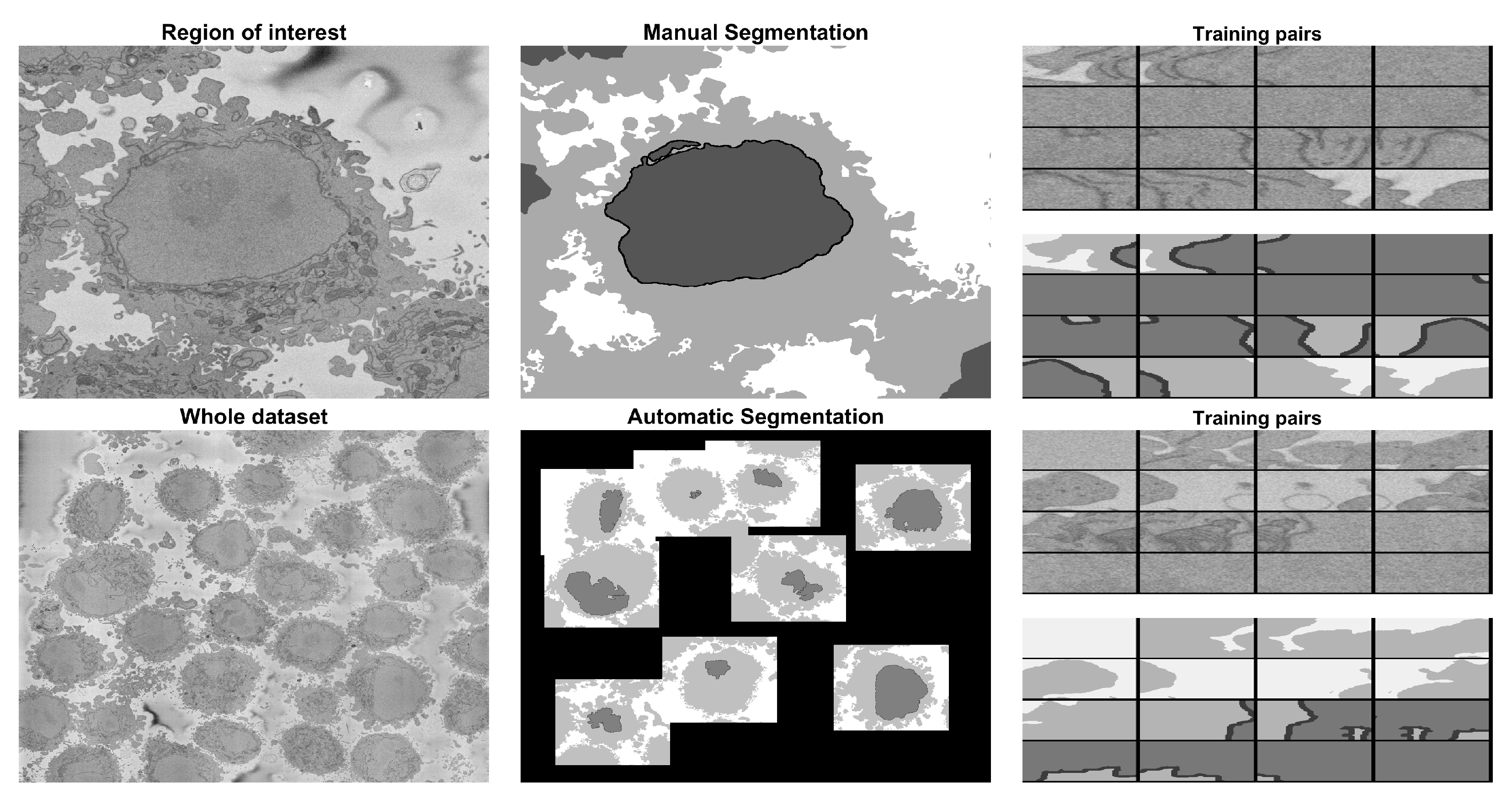
- A methodology to automatically generate a ground truth using a traditional image processing algorithm is proposed. This ground truth was used to generate training pairs that were later used to train a U-Net. The ground truth was obtained from several cells in several slices.
- Data, code and ground truth were publicly released through Empiar, GitHub and Zenodo.
2. Materials and Methods
2.1. HeLa Cells Preparation and Acquisition
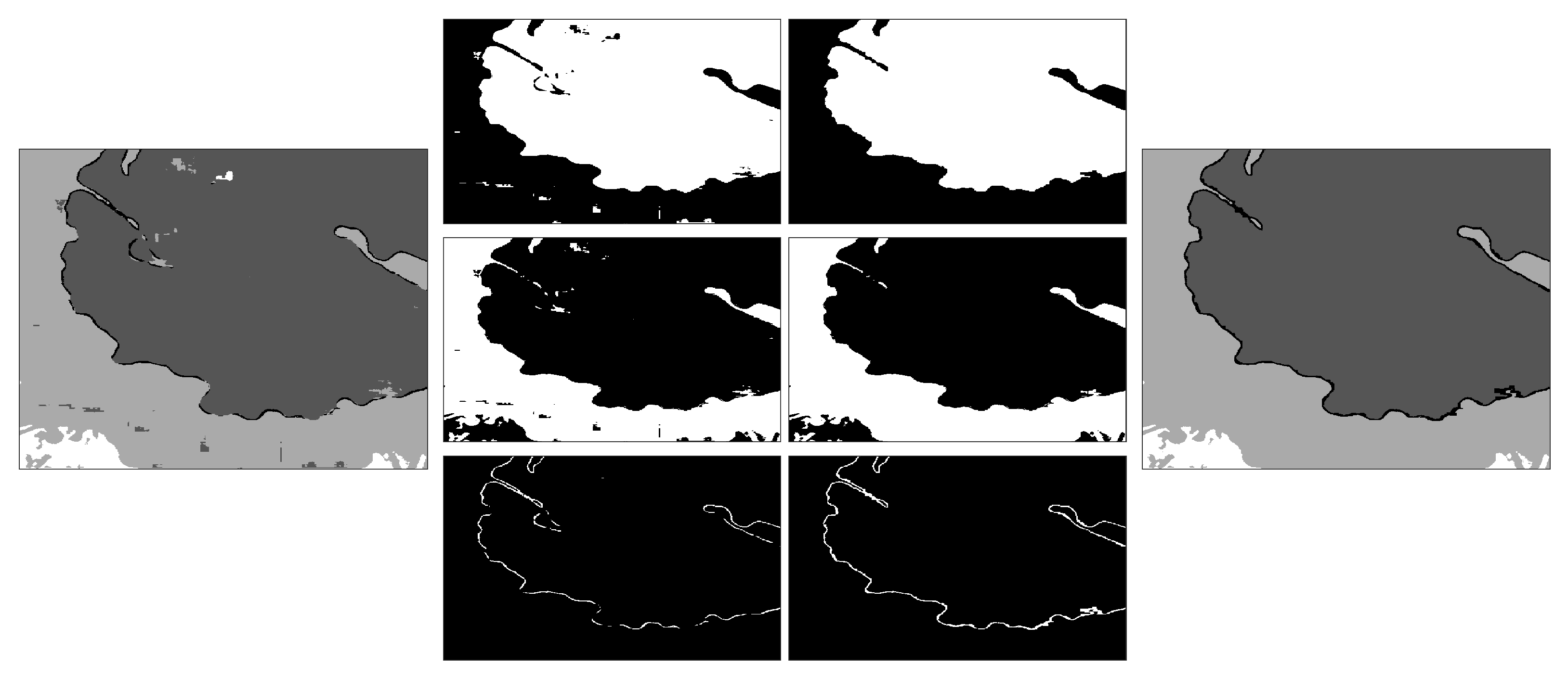
2.2. Ground Truth (GT)
2.3. Traditional Image Processing Segmentation Algorithm
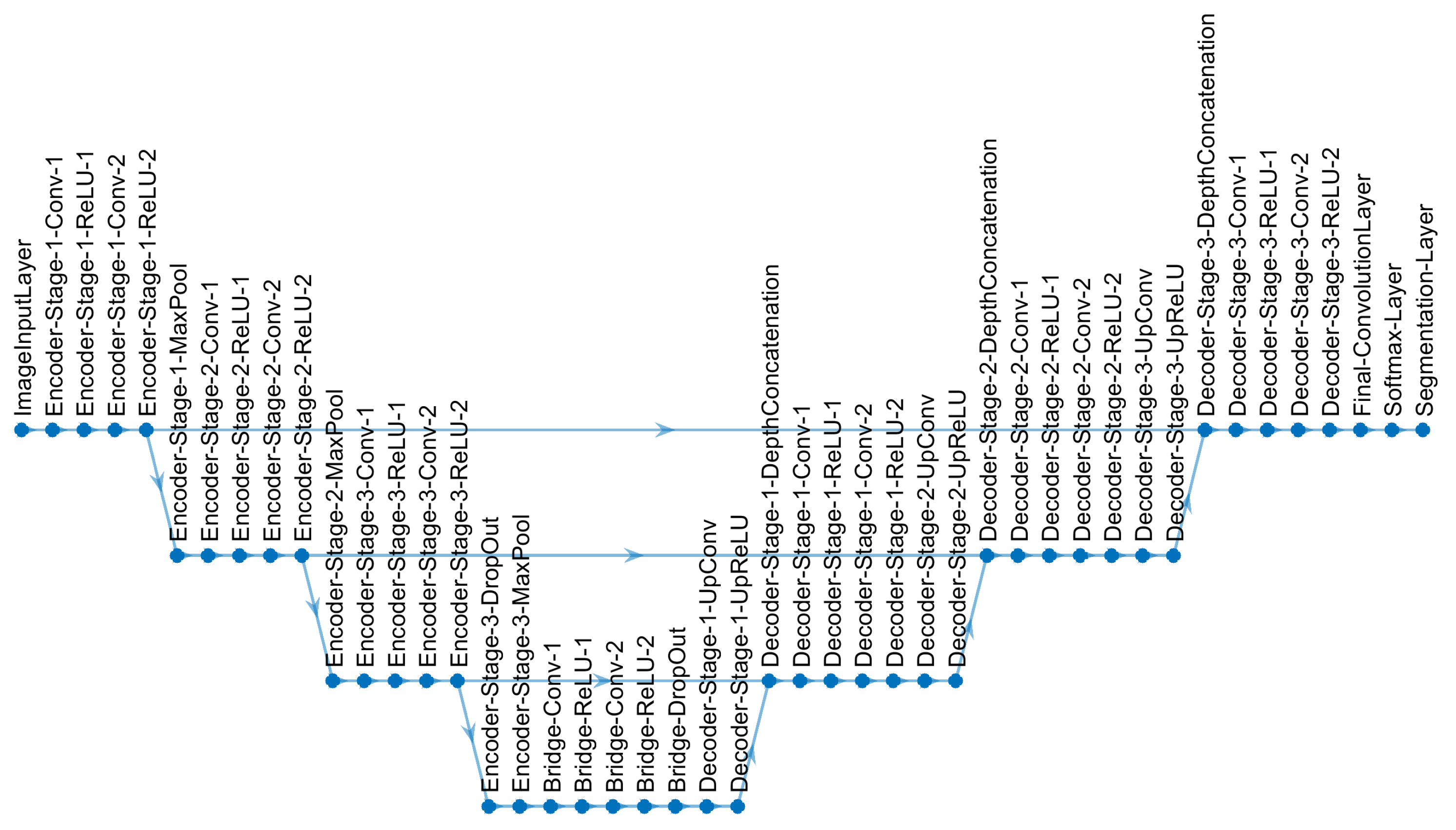
2.4. U-Net Architecture
2.5. U-Net Training Data, Segmentation and Post-Processing
- 1.
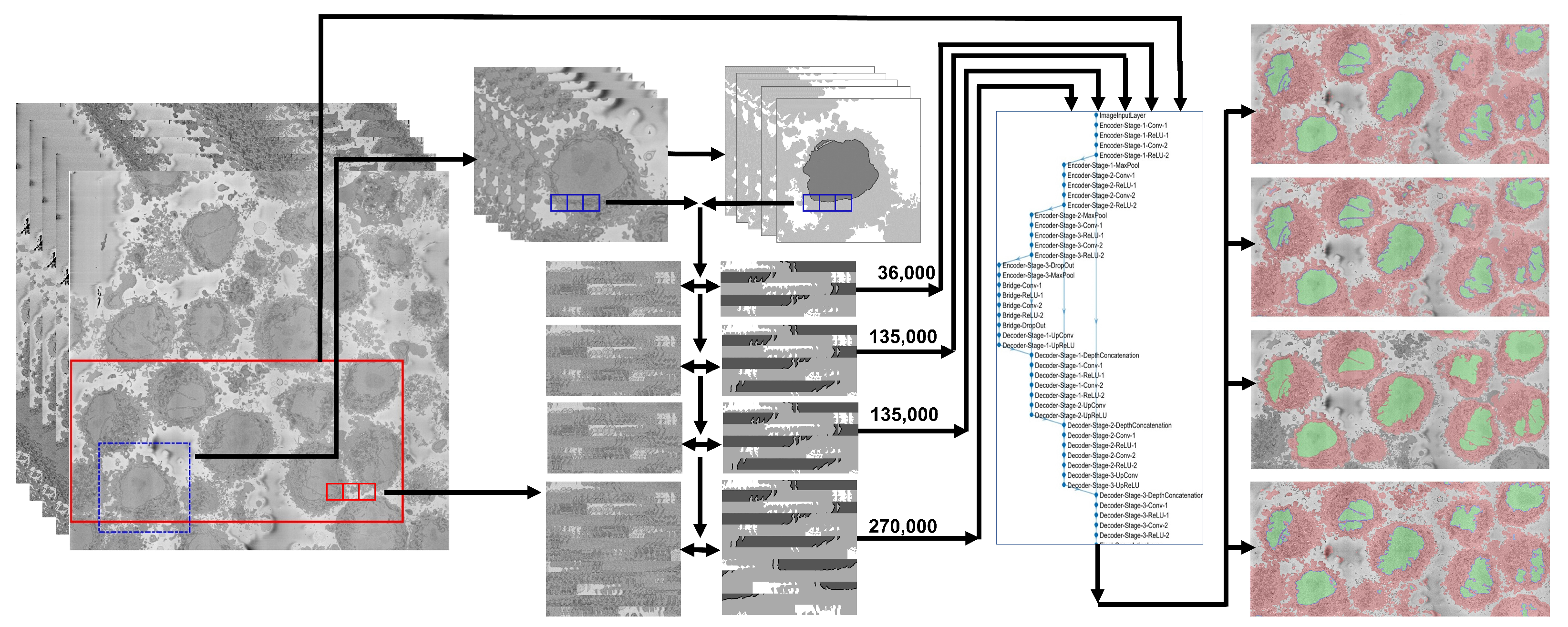
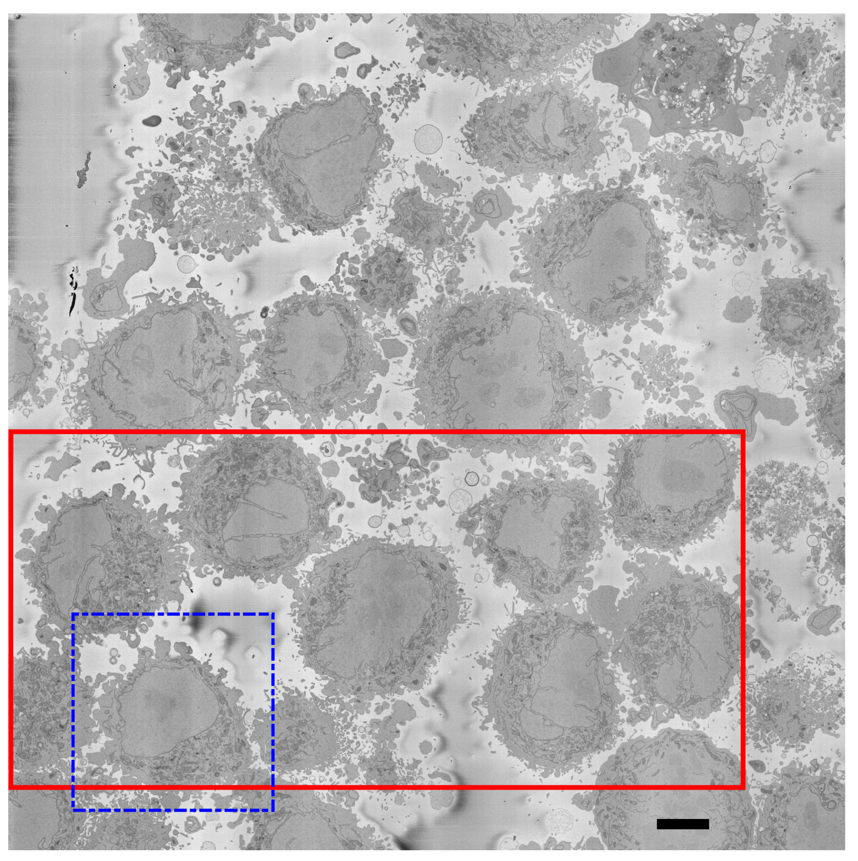
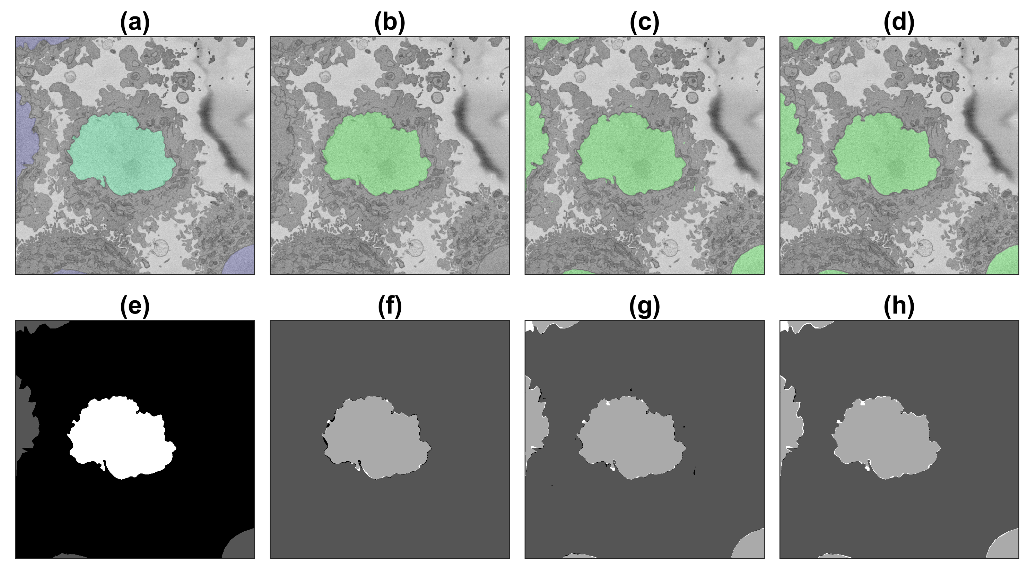
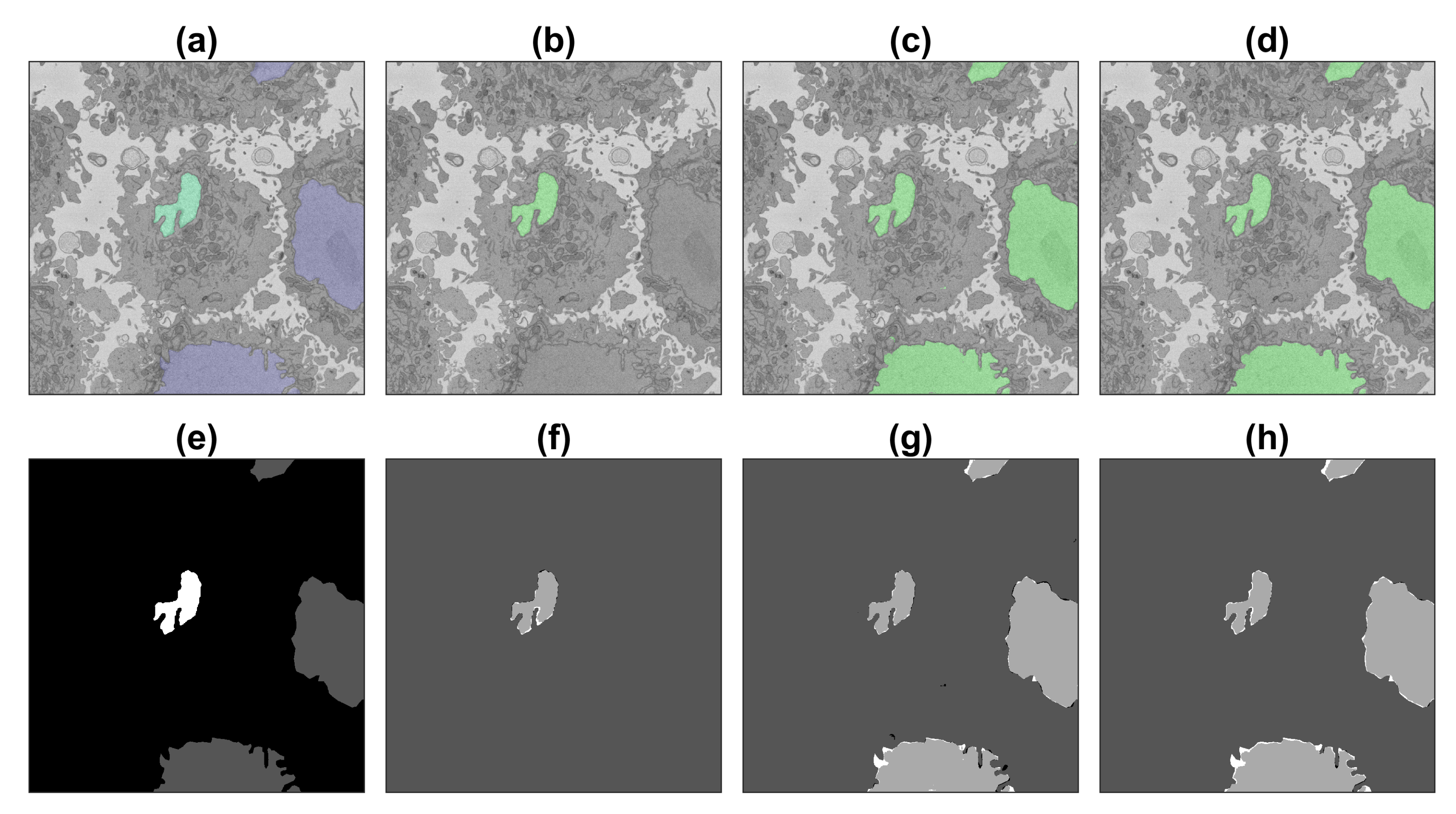
- A total of 36,000 pairs from manually delineated GT from a single cell, evaluated with a single cell in the GT. Pairs of patches of images and labels of size with 50% overlap were generated from 40 alternate slices of the central region of the cell (101:2:180). For one image, there were patches and thus corresponded to 36,000 patches. Alternate slices were selected to exploit the similarity between neighboring slices. In this case, the ground truth included only the nucleus of the central cell visible in the ROI.
- 2.
- A total of 36,000 pairs from manually delineated GT from a single cell, evaluated with multiple cells in the GT. The same strategy was followed to generate 36,000 patches and labels from alternate slices of the central region of the cell (101:2:180), however, in this case, the ground truth included the nuclei of all cells visible in the ROI.
- 3.
- A total of 135,000 pairs from manually delineated GT from a single cell, evaluated with multiple cells in the GT. The pairs of patches of labels and data were extended to cover every other slice of the whole region of interest (1:2:300). The size was again with 50% overlap; therefore, in this case, there were 150 slices and 900 patches per slice, which provided 135,000 pairs of patches for data and labels.
- 4.
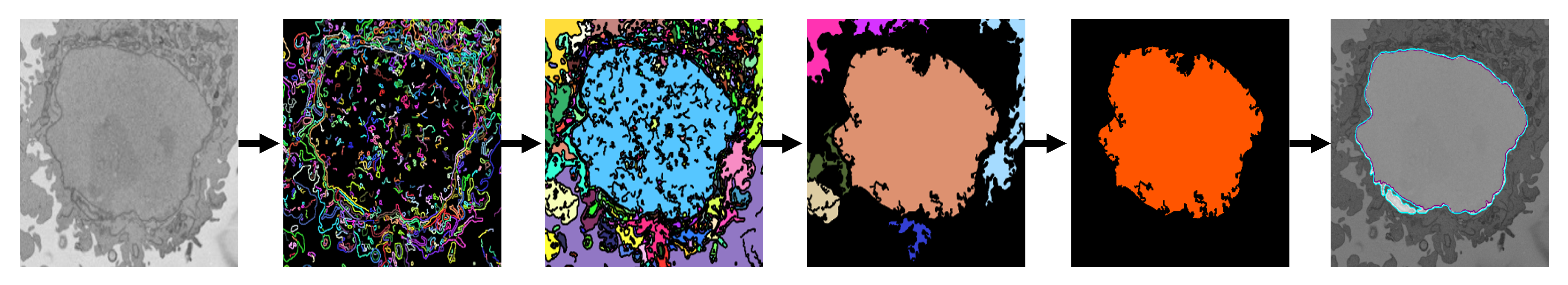
- A total of 135,000 pairs from automatically generated GT from multiple cells, evaluated visually. The training was extended beyond the region of interest by performing an automatic segmentation of the slices. This segmentation became a novel ground truth that was used to generate the same amount of pairs and in the previous strategy. The segmentation was performed with a traditional image processing segmentation algorithm [72] previously described. Fifteen non-contiguous slices were selected in the central region of the dataset (230:10:370). In each slice, the background was automatically segmented; distance transform was calculated to locate regions furthest from background, which corresponded to the cells. The 10 most salient cells were selected in each slice. A region was cropped, automatically segmented, and patches of with 50% overlap were generated. This generated 900 patches per cell, thus = 135,000. This training strategy was designed for the segmentation of the slices to compare the impact of segmenting with a U-Net trained on a single cell (even with a significant number of pairs) or with pairs from more than one cell.
- 5.
- A total of 270,000 pairs from manual (135,000) and automatic (135,000) GTs, evaluated visually. Finally, the patches generated in the two previous strategies, that is, the 135,000 from the single cell and the 135,000 from the whole dataset were combined for a total of 270,000.
2.6. Quantitative Comparisons
2.7. Hardware Details
3. Results and Discussion
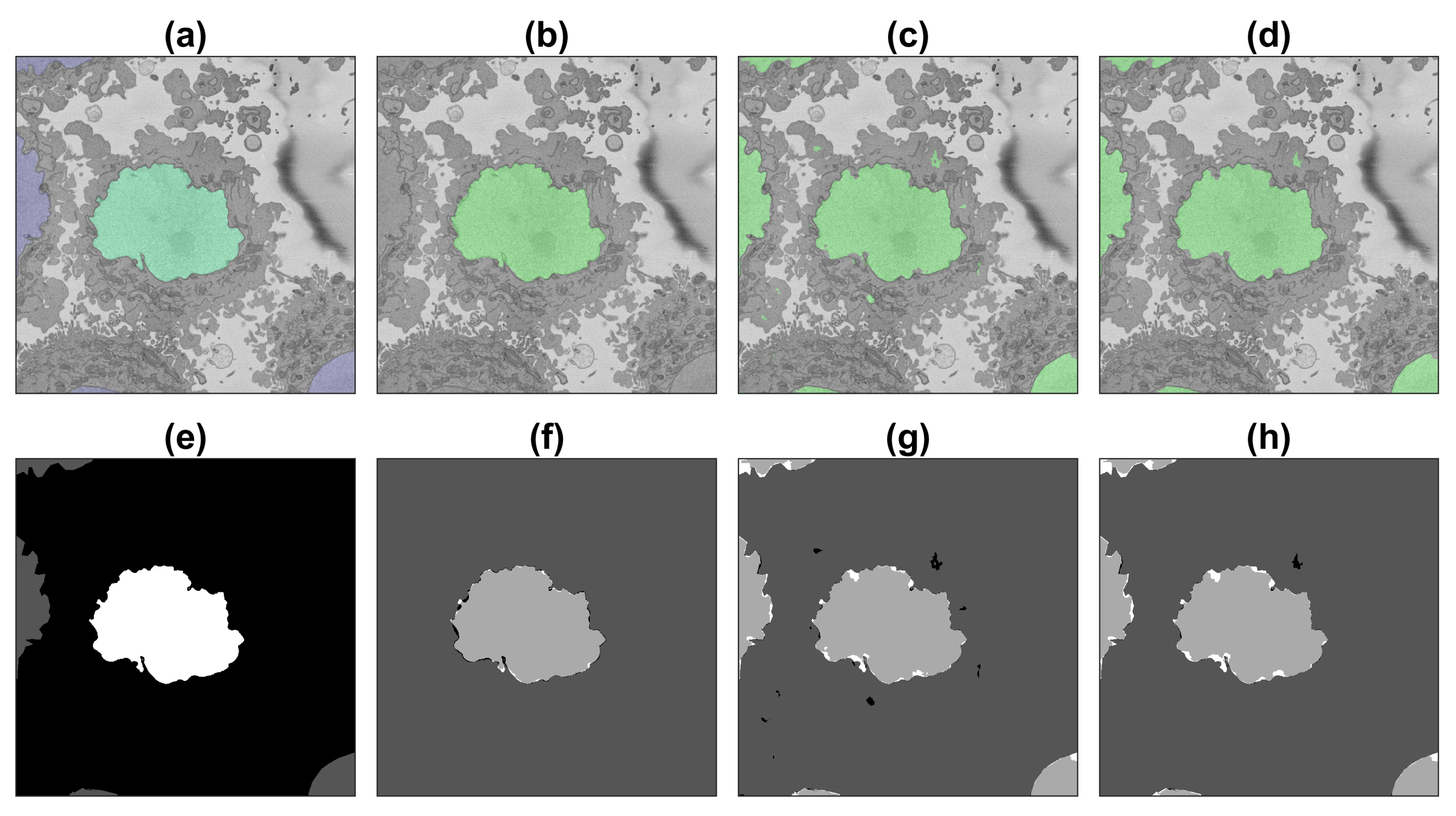
3.1. Results on the Region of Interest
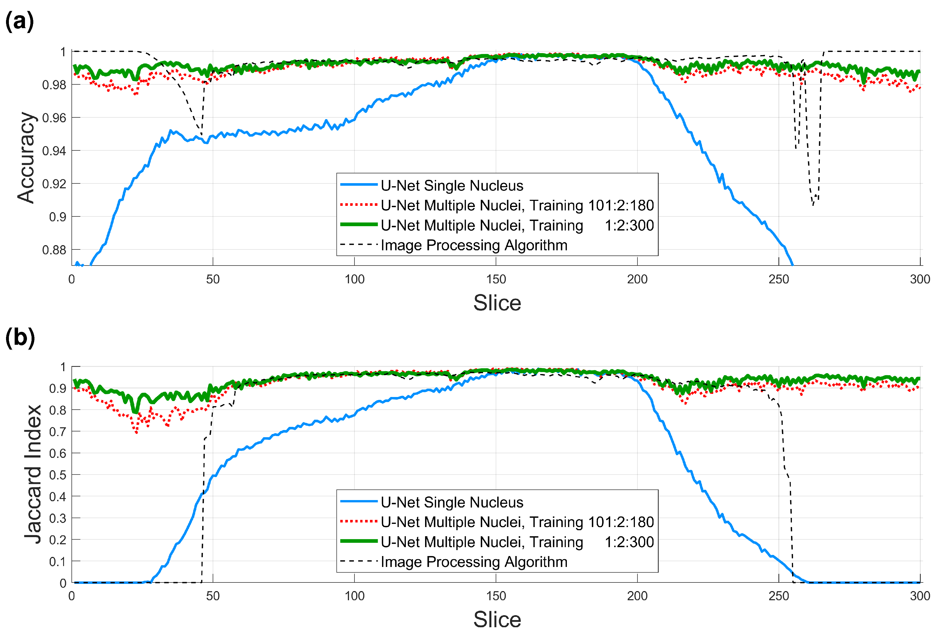
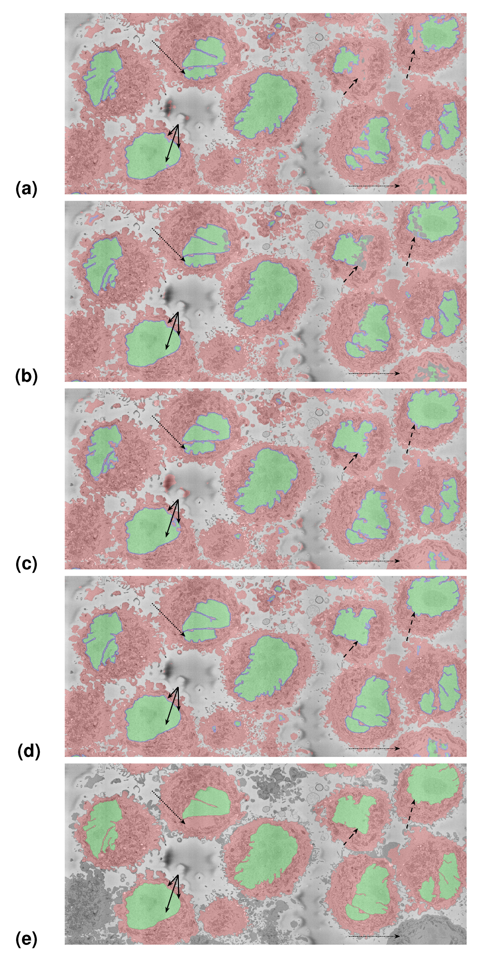
3.2. Results on the Slices
4. Conclusions
Author Contributions
Funding
Institutional Review Board Statement
Informed Consent Statement
Data Availability Statement
Acknowledgments
Conflicts of Interest
References
- Masters, J.R. HeLa cells 50 years on: The good, the bad and the ugly. Nat. Rev. Cancer 2002, 2, 315–319. [Google Scholar] [CrossRef] [PubMed]
- Rahbari, R.; Sheahan, T.; Modes, V.; Collier, P.; Macfarlane, C.; Badge, R.M. A novel L1 retrotransposon marker for HeLa cell line identification. BioTechniques 2009, 46, 277–284. [Google Scholar] [CrossRef] [PubMed]
- Yung, B.Y.; Bor, A.M. Identification of high-density lipoprotein in serum to determine anti-cancer efficacy of doxorubicin in HeLa cells. Int. J. Cancer 1992, 50, 951–957. [Google Scholar] [CrossRef]
- Zhang, S.L.; Wang, Y.S.; Zhou, T.; Yu, X.W.; Wei, Z.T.; Li, Y.L. Isolation and characterization of cancer stem cells from cervical cancer HeLa cells. Cytotechnology 2012, 64, 477–484. [Google Scholar] [CrossRef] [Green Version]
- Yang, J.; Zhang, B.; Qin, Z.; Li, S.; Xu, J.; Yao, Z.; Zhang, X.; Gonzalez, F.J.; Yao, X. Efflux excretion of bisdemethoxycurcumin-O-glucuronide in UGT1A1-overexpressing HeLa cells: Identification of breast cancer resistance protein (BCRP) and multidrug resistance-associated proteins 1 (MRP1) as the glucuronide transporters. Biofactors 2018, 44, 558–569. [Google Scholar] [CrossRef] [PubMed]
- Wang, L.; Qi, Y.; Xiong, Y.; Peng, Z.; Ma, Q.; Zhang, Y.; Song, J.; Zheng, J. Ezrin-Radixin-Moesin Binding Phosphoprotein 50 (EBP50) Suppresses the Metastasis of Breast Cancer and HeLa Cells by Inhibiting Matrix Metalloproteinase-2 Activity. Anticancer Res. 2017, 37, 4353–4360. [Google Scholar] [PubMed] [Green Version]
- Zukić, S.; Maran, U. Modelling of antiproliferative activity measured in HeLa cervical cancer cells in a series of xanthene derivatives. SAR QSAR Environ. Res. 2020, 31, 905–921. [Google Scholar] [CrossRef] [PubMed]
- Yang, Z.; Ahn, H.J.; Nam, H.W. Gefitinib inhibits the growth of Toxoplasma gondii in HeLa cells. Korean J. Parasitol. 2014, 52, 439–441. [Google Scholar] [CrossRef] [Green Version]
- Sanfelice, R.A.; Machado, L.F.; Bosqui, L.R.; Miranda-Sapla, M.M.; Tomiotto-Pellissier, F.; de Alcântara Dalevedo, G.; Ioris, D.; Reis, G.F.; Panagio, L.A.; Navarro, I.T.; et al. Activity of rosuvastatin in tachyzoites of Toxoplasma gondii (RH strain) in HeLa cells. Exp Parasitol 2017, 181, 75–81. [Google Scholar] [CrossRef]
- Zhang, Z.; Gu, H.; Li, Q.; Zheng, J.; Cao, S.; Weng, C.; Jia, H. GABARAPL2 Is Critical for Growth Restriction of Toxoplasma gondii in HeLa Cells Treated with Gamma Interferon. Infect. Immun. 2020, 88, e00054-20. [Google Scholar] [CrossRef]
- Pan, L.; Yang, Y.; Chen, X.; Zhao, M.; Yao, C.; Sheng, K.; Yang, Y.; Ma, G.; Du, A. Host autophagy limits Toxoplasma gondii proliferation in the absence of IFN-γ by affecting the hijack of Rab11A-positive vesicles. Front. Microbiol. 2022, 13, 1052779. [Google Scholar] [CrossRef] [PubMed]
- Tominaga, M.; Kumagai, E.; Harada, S. Effect of electrical stimulation on HIV-1-infected HeLa cells cultured on an electrode surface. Appl. Microbiol. Biotechnol. 2003, 61, 447–450. [Google Scholar] [CrossRef] [PubMed]
- Zheng, Y.; Zhou, H.; Zhang, C.; He, Y.; Li, H.; Chen, Z.; Liu, M. The apoptosis-inducing effects of HIV Vpr recombinant eukaryotic expression vectors with different mutation sites on transfected Hela cells. Curr. HIV Res. 2009, 7, 519–525. [Google Scholar] [CrossRef] [PubMed]
- Chesebro, B.; Wehrly, K.; Metcalf, J.; Griffin, D.E. Use of a new CD4-positive HeLa cell clone for direct quantitation of infectious human immunodeficiency virus from blood cells of AIDS patients. J. Infect. Dis. 1991, 163, 64–70. [Google Scholar] [CrossRef] [PubMed]
- Ekama, S.O.; Ilomuanya, M.O.; Azubuike, C.P.; Ayorinde, J.B.; Ezechi, O.C.; Igwilo, C.I.; Salako, B.L. Enzyme Responsive Vaginal Microbicide Gels Containing Maraviroc and Tenofovir Microspheres Designed for Acid Phosphatase-Triggered Release for Pre-Exposure Prophylaxis of HIV-1: A Comparative Analysis of a Bigel and Thermosensitive Gel. Gels 2021, 8, 15. [Google Scholar] [CrossRef] [PubMed]
- Zhang, B.; Liu, J.Y.; Pan, J.S.; Han, S.P.; Yin, X.X.; Wang, B.; Hu, G. Combined treatment of ionizing radiation with genistein on cervical cancer HeLa cells. J. Pharmacol. Sci. 2006, 102, 129–135. [Google Scholar] [CrossRef] [PubMed] [Green Version]
- Ziegler, W.; Birkenfeld, P.; Trott, K.R. The effect of combined treatment of HeLa cells with actinomycin D and radiation upon survival and recovery from radiation damage. Radiother. Oncol. 1987, 10, 141–148. [Google Scholar] [CrossRef]
- Zinberg, N.; Kohn, A. Dimethyl sulfoxide protection of HeLa cells against ionizing radiation during the growth cycle. Isr. J. Med. Sci. 1971, 7, 719–723. [Google Scholar]
- Zhu, C.; Wang, X.; Li, P.; Zhu, Y.; Sun, Y.; Hu, J.; Liu, H.; Sun, X. Developing a Peptide That Inhibits DNA Repair by Blocking the Binding of Artemis and DNA Ligase IV to Enhance Tumor Radiosensitivity. Int. J. Radiat. Oncol. 2021, 111, 515–527. [Google Scholar] [CrossRef]
- Skloot, R. The Immortal Life of Henrietta Lacks; Crown: New York, NY, USA, 2010. [Google Scholar]
- Rohde, G.K.; Ribeiro, A.J.S.; Dahl, K.N.; Murphy, R.F. Deformation-based nuclear morphometry: Capturing nuclear shape variation in HeLa cells. Cytometry. Part A J. Int. Soc. Anal. Cytol. 2008, 73, 341–350. [Google Scholar] [CrossRef]
- Suzuki, R.; Hotta, K.; Oka, K. Spatiotemporal quantification of subcellular ATP levels in a single HeLa cell during changes in morphology. Sci. Rep. 2015, 5, 16874. [Google Scholar] [CrossRef] [PubMed] [Green Version]
- Van Peteghem, M.C.; Mareel, M.M. Alterations in shape, surface structure and cytoskeleton of HeLa cells during monolayer culture. Arch. Biol. 1978, 89, 67–87. [Google Scholar]
- Welter, D.A.; Black, D.A.; Hodge, L.D. Nuclear reformation following metaphase in HeLa S3 cells: Three-dimensional visualization of chromatid rearrangements. Chromosoma 1985, 93, 57–68. [Google Scholar] [CrossRef] [PubMed]
- Bajcsy, P.; Cardone, A.; Chalfoun, J.; Halter, M.; Juba, D.; Kociolek, M.; Majurski, M.; Peskin, A.; Simon, C.; Simon, M.; et al. Survey statistics of automated segmentations applied to optical imaging of mammalian cells. BMC Bioinform. 2015, 16, 330. [Google Scholar] [CrossRef] [Green Version]
- Perez, A.; Seyedhosseini, M.; Deerinck, T.; Bushong, E.; Panda, S.; Tasdizen, T.; Ellisman, M. A workflow for the automatic segmentation of organelles in electron microscopy image stacks. Front. Neuroanat. 2014, 8, 1–13. [Google Scholar] [CrossRef]
- Wilke, S.; Antonios, J.; Bushong, E.; Badkoobehi, A.; Malek, E.; Hwang, M. Deconstructing complexity: Serial block-face electron microscopic analysis of the hippocampal mossy fiber synapse. J. Neurosci. 2013, 33, 507–522. [Google Scholar] [CrossRef] [PubMed] [Green Version]
- Bohorquez, D.; Samsa, L.; Roholt, A.; Medicetty, S.; Chandra, R.; Liddle, R. An enteroendocrine cell-enteric glia connection revealed by 3D electron microscopy. PLoS ONE 2014, 9, e89881. [Google Scholar] [CrossRef] [PubMed] [Green Version]
- Gurcan, M.N.; Boucheron, L.; Can, A.; Madabhushi, A.; Rajpoot, N.; Yener, B. Histopathological Image Analysis: A Review. IEEE Rev. Biomed. Eng. 2009, 2, 147–171. [Google Scholar] [CrossRef] [Green Version]
- Wang, Z.; Li, H. Generalizing cell segmentation and quantification. BMC Bioinform. 2017, 18, 189. [Google Scholar] [CrossRef] [Green Version]
- Pal, N.R.; Pal, S.R. A Review on Image Segmentation Techniques. Pattern Recognit. 1993, 26, 1277–1293. [Google Scholar] [CrossRef]
- Kapur, T. Model Based Three Dimensional Medical Image Segmentation. Ph.D. Thesis, AI Lab, Massachusetts Institute of Technology, Cambridge, MA, USA, 1999. [Google Scholar]
- Suri, J.S. Two-Dimensional Fast Magnetic Resonance Brain Segmentation. IEEE Eng. Med. Biol. 2001, 20, 84–95. [Google Scholar] [CrossRef] [PubMed]
- Zulfira, F.Z.; Suyanto, S.; Septiarini, A. Segmentation technique and dynamic ensemble selection to enhance glaucoma severity detection. Comput. Biol. Med. 2021, 139, 104951. [Google Scholar] [CrossRef] [PubMed]
- Zibrandtsen, I.C.; Kjaer, T.W. Fully automatic peak frequency estimation of the posterior dominant rhythm in a large retrospective hospital EEG cohort. Clin. Neurophysiol. Pract. 2021, 6, 1–9. [Google Scholar] [CrossRef] [PubMed]
- Xiong, F.; Zhang, Z.; Ling, Y.; Zhang, J. Image thresholding segmentation based on weighted Parzen-window and linear programming techniques. Sci. Rep. 2022, 12, 13635. [Google Scholar] [CrossRef]
- Held, K.; Kops, E.R.; Krause, B.J.; Wells, W.M.; Kikinis, R.; Muller-Gartner, H.W. Markov Random Field Segmentation of Brain MR Images. IEEE Trans. Med. Imaging 1997, 16, 6. [Google Scholar] [CrossRef] [Green Version]
- Zhang, Y.; Brady, M.; Smith, S. Segmentation of brain MR Images through a hidden Markov random field model and expectation maximization algorithm. IEEE Trans. Med. Imaging 2001, 20, 45–57. [Google Scholar] [CrossRef]
- Zhang, Z.; Zhao, T.; Gay, H.; Zhang, W.; Sun, B. ARPM-net: A novel CNN-based adversarial method with Markov random field enhancement for prostate and organs at risk segmentation in pelvic CT images. Med. Phys. 2020, 48, 227–237. [Google Scholar] [CrossRef]
- Ren, X.; Malik, J. Learning a classification model for segmentation. In Proceedings of the Ninth IEEE International Conference on Computer Vision, Nice, France, 13–16 October 2003. [Google Scholar] [CrossRef] [Green Version]
- Stutz, D.; Hermans, A.; Leibe, B. Superpixels: An evaluation of the state-of-the-art. Comput. Vis. Image Underst. 2018, 166, 1–27. [Google Scholar] [CrossRef] [Green Version]
- Albayrak, A.; Bilgin, G. Automatic cell segmentation in histopathological images via two-staged superpixel-based algorithms. Med. Biol. Eng. Comput. 2018, 57, 653–665. [Google Scholar] [CrossRef]
- Vincent, L.; Soille, P. Watersheds in digital spaces: An efficient algorithm based on immersion simulations. IEEE Trans. Pattern Anal. Mach. Intell. 1991, 13, 583–598. [Google Scholar] [CrossRef] [Green Version]
- Cousty, J.; Bertrand, G.; Najman, L.; Couprie, M. Watershed Cuts: Thinnings, Shortest Path Forests, and Topological Watersheds. IEEE Trans. Pattern Anal. Mach. Intell. 2010, 32, 925–939. [Google Scholar] [CrossRef] [PubMed] [Green Version]
- Gamarra, M.; Zurek, E.; Escalante, H.J.; Hurtado, L.; San-Juan-Vergara, H. Split and merge watershed: A two-step method for cell segmentation in fluorescence microscopy images. Biomed. Signal Process. Control 2019, 53, 101575. [Google Scholar] [CrossRef] [PubMed]
- Zumbado-Corrales, M.; Esquivel-Rodríguez, J. EvoSeg: Automated Electron Microscopy Segmentation through Random Forests and Evolutionary Optimization. Biomimetics 2021, 6, 37. [Google Scholar] [CrossRef] [PubMed]
- Chan, T.; Vese, L. Active contours without edges. IEEE Trans. Image Process. 2001, 10, 266–277. [Google Scholar] [CrossRef] [PubMed] [Green Version]
- Ciecholewski, M.; Spodnik, J. Semi–Automatic Corpus Callosum Segmentation and 3D Visualization Using Active Contour Methods. Symmetry 2018, 10, 589. [Google Scholar] [CrossRef] [Green Version]
- Zhu, X.; Wei, Y.; Lu, Y.; Zhao, M.; Yang, K.; Wu, S.; Zhang, H.; Wong, K.K. Comparative analysis of active contour and convolutional neural network in rapid left-ventricle volume quantification using echocardiographic imaging. Comput. Methods Programs Biomed. 2021, 199, 105914. [Google Scholar] [CrossRef]
- Song, T.H.; Sanchez, V.; EIDaly, H.; Rajpoot, N.M. Dual-Channel Active Contour Model for Megakaryocytic Cell Segmentation in Bone Marrow Trephine Histology Images. IEEE Trans. Biomed. Eng. 2017, 64, 2913–2923. [Google Scholar] [CrossRef] [Green Version]
- Arafat, Y.; Reyes-Aldasoro, C.C. Computational Image Analysis Techniques, Programming Languages and Software Platforms Used in Cancer Research: A Scoping Review. In Proceedings of the Medical Image Understanding and Analysis; Yang, G., Aviles-Rivero, A., Roberts, M., Schönlieb, C.B., Eds.; Lecture Notes in Computer Science; Springer International Publishing: Cham, Switzerland, 2022; Volume 13413, pp. 833–847. [Google Scholar]
- Michael, E.; Ma, H.; Li, H.; Kulwa, F.; Li, J. Breast Cancer Segmentation Methods: Current Status and Future Potentials. BioMed Res. Int. 2021, 2021, 9962109. [Google Scholar] [CrossRef]
- Vicar, T.; Balvan, J.; Jaros, J.; Jug, F.; Kolar, R.; Masarik, M.; Gumulec, J. Cell segmentation methods for label-free contrast microscopy: Review and comprehensive comparison. BMC Bioinform. 2019, 20, 360. [Google Scholar] [CrossRef]
- Jones, M.L.; Spiers, H. The crowd storms the ivory tower. Nat. Methods 2018, 15, 579–580. [Google Scholar] [CrossRef]
- Tripathi, S.; Chandra, S.; Agrawal, A.; Tyagi, A.; Rehg, J.M.; Chari, V. Learning to Generate Synthetic Data via Compositing. In Proceedings of the CVPR 2019, Long Beach, CA, USA, 16–20 June 2019; pp. 461–470. [Google Scholar]
- Such, F.P.; Rawal, A.; Lehman, J.; Stanley, K.; Clune, J. Generative Teaching Networks: Accelerating Neural Architecture Search by Learning to Generate Synthetic Training Data. In Proceedings of the 37th International Conference on Machine Learning, Virtual Event, 13–18 July 2020; PMLR: Brookline, MA, USA, 2020; pp. 9206–9216. [Google Scholar]
- Chen, X.; Mersch, B.; Nunes, L.; Marcuzzi, R.; Vizzo, I.; Behley, J.; Stachniss, C. Automatic Labeling to Generate Training Data for Online LiDAR-Based Moving Object Segmentation. IEEE Robot. Autom. Lett. 2022, 7, 6107–6114. [Google Scholar] [CrossRef]
- Schmitz, S.; Weinmann, M.; Weidner, U.; Hammer, H.; Thiele, A. Automatic generation of training data for land use and land cover classification by fusing heterogeneous data sets. Publ. Der Dtsch. Ges. Für Photogramm. Fernerkund. Und Geoinf. 2020, 29, 73–86. [Google Scholar]
- Voelsen, M.; Torres, D.L.; Feitosa, R.Q.; Rottensteiner, F.; Heipke, C. Investigations on Feature Similarity and the Impact of Training Data for Land Cover Classification. ISPRS Ann. Photogramm. Remote Sens. Spat. Inf. Sci. 2021, 3, 181–189. [Google Scholar] [CrossRef]
- Wen, T.; Tong, B.; Liu, Y.; Pan, T.; Du, Y.; Chen, Y.; Zhang, S. Review of research on the instance segmentation of cell images. Comput. Methods Programs Biomed. 2022, 227, 107211. [Google Scholar] [CrossRef] [PubMed]
- Zhang, L.; Jia, Z.; Leng, X.; Ma, F. Artificial Intelligence Algorithm-Based Ultrasound Image Segmentation Technology in the Diagnosis of Breast Cancer Axillary Lymph Node Metastasis. J. Healthc. Eng. 2021, 2021, 8830260. [Google Scholar] [CrossRef]
- Yang, M.; Zhang, Y.; Chen, H.; Wang, W.; Ni, H.; Chen, X.; Li, Z.; Mao, C. AX-Unet: A Deep Learning Framework for Image Segmentation to Assist Pancreatic Tumor Diagnosis. Front. Oncol. 2022, 12, 894970. [Google Scholar] [CrossRef] [PubMed]
- Tsochatzidis, L.; Koutla, P.; Costaridou, L.; Pratikakis, I. Integrating segmentation information into CNN for breast cancer diagnosis of mammographic masses. Comput. Methods Programs Biomed. 2021, 200, 105913. [Google Scholar] [CrossRef]
- Tahir, H.B.; Washington, S.; Yasmin, S.; King, M.; Haque, M.M. Influence of segmentation approaches on the before-after evaluation of engineering treatments: A hypothetical treatment approach. Accid. Anal. Prev. 2022, 176, 106795. [Google Scholar] [CrossRef] [PubMed]
- Ostroff, L.; Zeng, H. Electron Microscopy at Scale. Cell 2015, 162, 474–475. [Google Scholar] [CrossRef] [Green Version]
- Peddie, C.; Collinson, L. Exploring the third dimension: Volume electron microscopy comes of age. Micron 2014, 61, 9–19. [Google Scholar] [CrossRef]
- Tsai, W.T.; Hassan, A.; Sarkar, P.; Correa, J.; Metlagel, Z.; Jorgens, D.M.; Auer, M. From voxels to knowledge: A practical guide to the segmentation of complex electron microscopy 3D-data. J. Vis. Exp. 2014, 90, e51673. [Google Scholar] [CrossRef] [Green Version]
- Russell, M.R.; Lerner, T.R.; Burden, J.J.; Nkwe, D.O.; Pelchen-Matthews, A.; Domart, M.C.; Durgan, J.; Weston, A.; Jones, M.L.; Peddie, C.J.; et al. 3D correlative light and electron microscopy of cultured cells using serial blockface scanning electron microscopy. J. Cell Sci. 2017, 130, 278–291. [Google Scholar] [CrossRef] [PubMed] [Green Version]
- LeCun, Y.; Bengio, Y.; Hinton, G. Deep learning. Nature 2015, 521, 436–444. [Google Scholar] [CrossRef] [PubMed]
- Spiers, H.; Songhurst, H.; Nightingale, L.; de Folter, J.; Zooniverse Volunteer Community, Z.; Hutchings, R.; Peddie, C.J.; Weston, A.; Strange, A.; Hindmarsh, S.; et al. Deep learning for automatic segmentation of the nuclear envelope in electron microscopy data, trained with volunteer segmentations. Traffic 2021, 22, 240–253. [Google Scholar] [CrossRef]
- Karabag, C.; Jones, M.L.; Peddie, C.J.; Weston, A.E.; Collinson, L.M.; Reyes-Aldasoro, C.C. Automated Segmentation of HeLa Nuclear Envelope from Electron Microscopy Images. In Proceedings of the Medical Image Understanding and Analysis, Southampton, UK, 9–11 July 2018; Springer International Publishing: Cham, Switzerland, 2018; pp. 241–250. [Google Scholar] [CrossRef] [Green Version]
- Karabağ, C.; Jones, M.L.; Peddie, C.J.; Weston, A.E.; Collinson, L.M.; Reyes-Aldasoro, C.C. Segmentation and Modelling of the Nuclear Envelope of HeLa Cells Imaged with Serial Block Face Scanning Electron Microscopy. J. Imaging 2019, 5, 75. [Google Scholar] [CrossRef] [PubMed] [Green Version]
- Karabağ, C.; Jones, M.L.; Peddie, C.J.; Weston, A.E.; Collinson, L.M.; Reyes-Aldasoro, C.C. Semantic segmentation of HeLa cells: An objective comparison between one traditional algorithm and four deep-learning architectures. PLoS ONE 2020, 15, e0230605. [Google Scholar] [CrossRef] [PubMed]
- Jones, M.; Songhurst, H.; Peddie, C.; Weston, A.; Spiers, H.; Lintott, C.; Collinson, L.M. Harnessing the Power of the Crowd for Bioimage Analysis. Microsc. Microanal. 2019, 25, 1372–1373. [Google Scholar] [CrossRef] [Green Version]
- Karabağ, C.; Jones, M.L.; Reyes-Aldasoro, C.C. Volumetric Semantic Instance Segmentation of the Plasma Membrane of HeLa Cells. J. Imaging 2021, 7, 93. [Google Scholar] [CrossRef]
- Ronneberger, O.; Fischer, P.; Brox, T. U-Net: Convolutional Networks for Biomedical Image Segmentation. arXiv 2015, arXiv:1505.04597. [Google Scholar]
- Deerinck, T.J.; Bushong, E.A.; Thor, A.; Ellisman, M.H. NCMIR: A New Protocol for Preparation of Biological Specimens for Serial Block-Face SEM Microscopy. 2010. Available online: https://ncmir.ucsd.edu/sbem-protocol (accessed on 23 February 2023).
- Iudin, A.; Korir, P.K.; Salavert-Torres, J.; Kleywegt, G.J.; Patwardhan, A. EMPIAR: A public archive for raw electron microscopy image data. Nat. Methods 2016, 13, 387–388. [Google Scholar] [CrossRef]
- Canny, J. A Computational Approach to Edge Detection. IEEE Trans. Pattern Anal. Mach. Intell. 1986, PAMI-8, 679–698. [Google Scholar] [CrossRef]
- Zhang, R.; Huang, L.; Xia, W.; Zhang, B.; Qiu, B.; Gao, X. Multiple supervised residual network for osteosarcoma segmentation in CT images. Comput. Med. Imaging Graph. 2018, 63, 1–8. [Google Scholar] [CrossRef] [PubMed]
- Zhou, T.; Dong, Y.; Lu, H.; Zheng, X.; Qiu, S.; Hou, S. APU-Net: An Attention Mechanism Parallel U-Net for Lung Tumor Segmentation. Biomed Res. Int. 2022, 2022, 5303651. [Google Scholar] [CrossRef] [PubMed]
- Zhao, H.; Niu, J.; Meng, H.; Wang, Y.; Li, Q.; Yu, Z. Focal U-Net: A Focal Self-attention based U-Net for Breast Lesion Segmentation in Ultrasound Images. In Proceedings of the 2022 44th Annual International Conference of the IEEE Engineering in Medicine & Biology Society (EMBC), Glasgow, UK, 11–15 July 2022; pp. 1506–1511. [Google Scholar]
- Mutaguchi, J.; Morooka, K.; Kobayashi, S.; Umehara, A.; Miyauchi, S.; Kinoshita, F.; Inokuchi, J.; Oda, Y.; Kurazume, R.; Eto, M. Artificial Intelligence for Segmentation of Bladder Tumor Cystoscopic Images Performed by U-Net with Dilated Convolution. J. Endourol. 2022, 36, 827–834. [Google Scholar] [CrossRef] [PubMed]
- Zhang, Y.; Chen, J.H.; Chang, K.T.; Park, V.Y.; Kim, M.J.; Chan, S.; Chang, P.; Chow, D.; Luk, A.; Kwong, T.; et al. Automatic Breast and Fibroglandular Tissue Segmentation in Breast MRI Using Deep Learning by a Fully-Convolutional Residual Neural Network U-Net. Acad. Radiol. 2019, 26, 1526–1535. [Google Scholar] [CrossRef] [PubMed]
- Zhao, B.; Chen, X.; Li, Z.; Yu, Z.; Yao, S.; Yan, L.; Wang, Y.; Liu, Z.; Liang, C.; Han, C. Triple U-net: Hematoxylin-aware nuclei segmentation with progressive dense feature aggregation. Med. Image Anal. 2020, 65, 101786. [Google Scholar] [CrossRef]
- Kingma, D.P.; Ba, J. Adam: A Method for Stochastic Optimization. arXiv 2014, arXiv:1412.6980. [Google Scholar]
- Jaccard, P. Étude comparative de la distribution florale dans une portion des Alpes et des Jura. Bull. Del La Société Vaudoise Des Sci. Nat. 1901, 37, 547–579. [Google Scholar]
- Futrega, M.; Milesi, A.; Marcinkiewicz, M.; Ribalta, P. Optimized U-Net for Brain Tumor Segmentation. In Brainlesion: Glioma, Multiple Sclerosis, Stroke and Traumatic Brain Injuries; Springer International Publishing: Berlin/Heidelberg, Germany, 2022; pp. 15–29. [Google Scholar] [CrossRef]
- Karabağ, C.; Verhoeven, J.; Miller, N.R.; Reyes-Aldasoro, C.C. Texture Segmentation: An Objective Comparison between Five Traditional Algorithms and a Deep-Learning U-Net Architecture. Appl. Sci. 2019, 9, 3900. [Google Scholar] [CrossRef] [Green Version]
- Jaffari, R.; Hashmani, M.A.; Reyes-Aldasoro, C.C. A Novel Focal Phi Loss for Power Line Segmentation with Auxiliary Classifier U-Net. Sensors 2021, 21, 2803. [Google Scholar] [CrossRef]
- Astono, I.P.; Welsh, J.S.; Chalup, S.; Greer, P. Optimisation of 2D U-Net Model Components for Automatic Prostate Segmentation on MRI. Appl. Sci. 2020, 10, 2601. [Google Scholar] [CrossRef] [Green Version]
- Li, S.; Xu, J.; Chen, R. U-Net Neural Network Optimization Method Based on Deconvolution Algorithm. In Neural Information Processing; Springer International Publishing: Berlin/Heidelberg, Germany, 2020; pp. 592–602. [Google Scholar] [CrossRef]
- Kirichev, M.M.; Slavov, T.S.; Momcheva, G.D. Fuzzy U-Net Neural Network Architecture Optimization for Image Segmentation. IOP Conf. Ser. Mater. Sci. Eng. 2021, 1031, 012077. [Google Scholar] [CrossRef]
- Chen, T.; Kornblith, S.; Norouzi, M.; Hinton, G. A Simple Framework for Contrastive Learning of Visual Representations. arXiv 2020, arXiv:2002.05709. [Google Scholar]
- Castro, E.; Cardoso, J.S.; Pereira, J.C. Elastic deformations for data augmentation in breast cancer mass detection. In Proceedings of the 2018 IEEE EMBS International Conference on Biomedical & Health Informatics (BHI), Las Vegas, NV, USA, 4–7 March 2018. [Google Scholar] [CrossRef]
- Chlap, P.; Min, H.; Vandenberg, N.; Dowling, J.; Holloway, L.; Haworth, A. A review of medical image data augmentation techniques for deep learning applications. J. Med. Imaging Radiat. Oncol. 2021, 65, 545–563. [Google Scholar] [CrossRef] [PubMed]


| U-Net Single Nucleus 36,000 Strategy 1 | U-Net Multiple Nuclei 36,000 Strategy 2 | U-Net Multiple Nuclei 135,000 Strategy 3 | Image Processing Algorithm | |
|---|---|---|---|---|
| Accuracy 1:300 | 0.9346 | 0.9895 | 0.9922 | 0.9926 |
| Accuracy 150:200 | 0.9966 | 0.9974 | 0.9971 | 0.9945 |
| Jaccard 1:300 | 0.5138 | 0.9158 | 0.9378 | 0.6436 |
| Jaccard 150:200 | 0.9712 | 0.9778 | 0.9760 | 0.9564 |
| Jaccard 60:150 | 0.8047 | 0.9579 | 0.9592 | 0.9565 |
Disclaimer/Publisher’s Note: The statements, opinions and data contained in all publications are solely those of the individual author(s) and contributor(s) and not of MDPI and/or the editor(s). MDPI and/or the editor(s) disclaim responsibility for any injury to people or property resulting from any ideas, methods, instructions or products referred to in the content. |
© 2023 by the authors. Licensee MDPI, Basel, Switzerland. This article is an open access article distributed under the terms and conditions of the Creative Commons Attribution (CC BY) license (https://creativecommons.org/licenses/by/4.0/).
Share and Cite
Karabağ, C.; Ortega-Ruíz, M.A.; Reyes-Aldasoro, C.C. Impact of Training Data, Ground Truth and Shape Variability in the Deep Learning-Based Semantic Segmentation of HeLa Cells Observed with Electron Microscopy. J. Imaging 2023, 9, 59. https://doi.org/10.3390/jimaging9030059
Karabağ C, Ortega-Ruíz MA, Reyes-Aldasoro CC. Impact of Training Data, Ground Truth and Shape Variability in the Deep Learning-Based Semantic Segmentation of HeLa Cells Observed with Electron Microscopy. Journal of Imaging. 2023; 9(3):59. https://doi.org/10.3390/jimaging9030059
Chicago/Turabian StyleKarabağ, Cefa, Mauricio Alberto Ortega-Ruíz, and Constantino Carlos Reyes-Aldasoro. 2023. "Impact of Training Data, Ground Truth and Shape Variability in the Deep Learning-Based Semantic Segmentation of HeLa Cells Observed with Electron Microscopy" Journal of Imaging 9, no. 3: 59. https://doi.org/10.3390/jimaging9030059