Figure 1.
An illustration of the training and validation loss curves. Training and validation losses decrease simultaneously until the fitting point. After that, the validation loss begins to rise while the training loss is still decreasing, i.e., the so-called overfitting. Overfitting is associated with good performance on the training data but poor generalisation to the validation/test data (cf. underfitting is associated with poor performance on the training data and poor generalisation to the validation data) [
12].
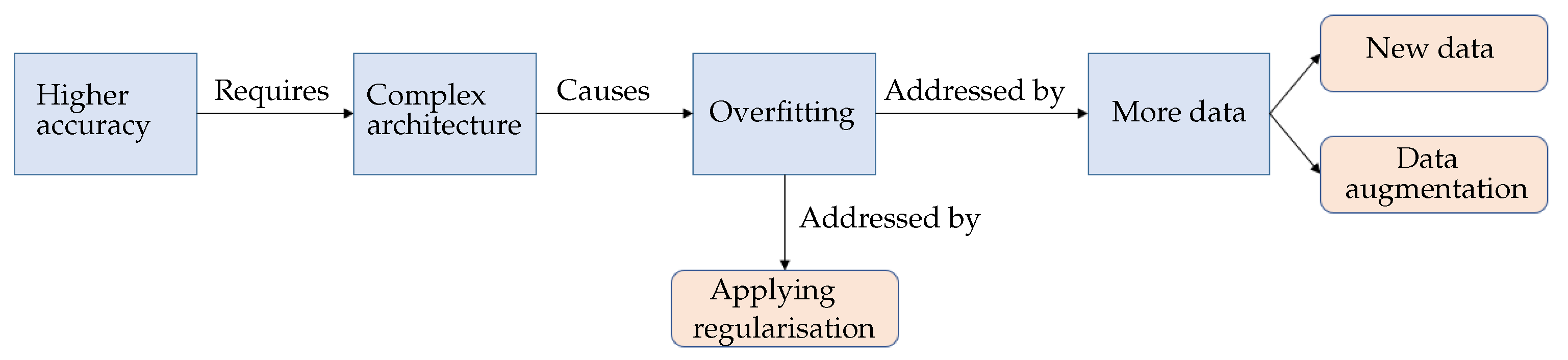
Figure 2.
Diagram illustrating the overfitting problem and its well-known solutions.
Figure 2.
Diagram illustrating the overfitting problem and its well-known solutions.
Figure 3.
Data augmentation (DA) taxonomy.
Figure 3.
Data augmentation (DA) taxonomy.
Figure 4.
Traditional rotation. Left and right: the given image (from the CIFAR-10 dataset) and the rotated image with a randomly rotated angle. Black areas appear in the corners of the rotated image and the corners in the given image are cut off in the rotated image.
Figure 4.
Traditional rotation. Left and right: the given image (from the CIFAR-10 dataset) and the rotated image with a randomly rotated angle. Black areas appear in the corners of the rotated image and the corners in the given image are cut off in the rotated image.
Figure 5.
Data augmentation by different types of rotation techniques. The left three figures in the first row show the “constant” technique, i.e., the traditional rotation (TR), resulting in black areas around the boundary. The RNR technique is used in the right three figures of the first row. The first three figures of the second row give the results of filling up the black areas by using RRR, and the right three figures use RWR. For each technique, three random angles were selected for rotation.
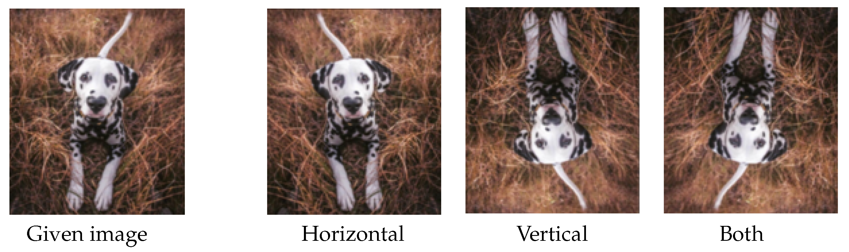
Figure 6.
Data augmentation by flipping. Images from left to right represent the given image, horizontally flipped image, vertically flipped image and the image flipped horizontally and vertically, respectively.
Figure 6.
Data augmentation by flipping. Images from left to right represent the given image, horizontally flipped image, vertically flipped image and the image flipped horizontally and vertically, respectively.
Figure 7.
Data augmentation by cropping. Left and right: the given image (from ImageNet) labelled as “Dog” and the cropped patch. It is clear that the “Dog” is no longer visible in the cropped patch.
Figure 7.
Data augmentation by cropping. Left and right: the given image (from ImageNet) labelled as “Dog” and the cropped patch. It is clear that the “Dog” is no longer visible in the cropped patch.
Figure 8.
Data augmentation by colour jittering. (a–d) represent the given image, and the augmented images by manipulating the colour saturation, brightness and contrast, respectively.
Figure 8.
Data augmentation by colour jittering. (a–d) represent the given image, and the augmented images by manipulating the colour saturation, brightness and contrast, respectively.
Figure 9.
Data augmentation by using kernels/filters.
Figure 9.
Data augmentation by using kernels/filters.
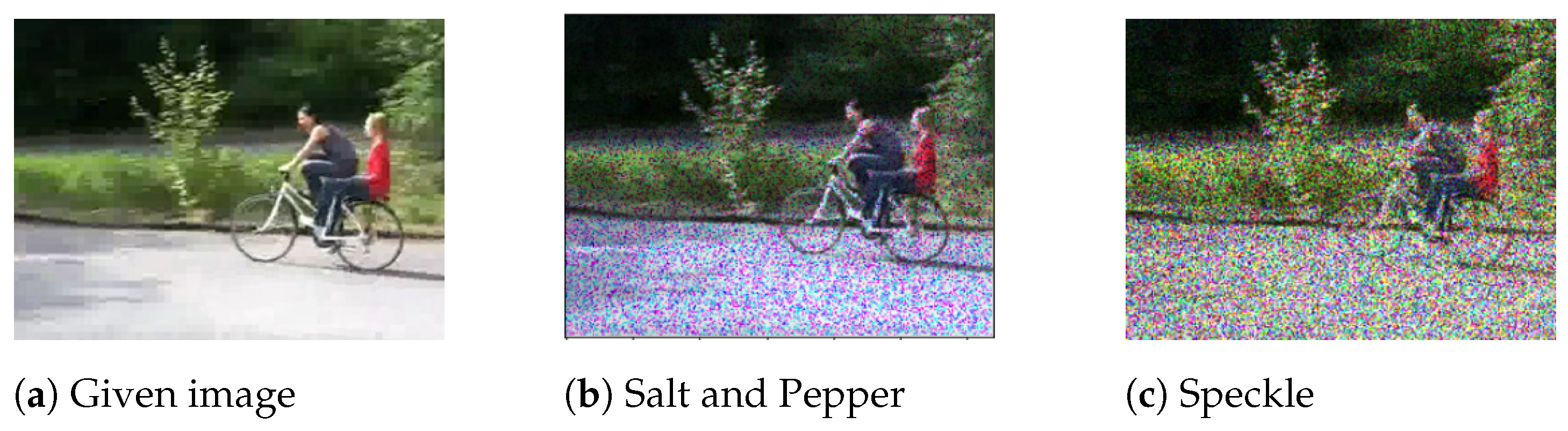
Figure 10.
Data augmentation by using noise transformation.
Figure 10.
Data augmentation by using noise transformation.
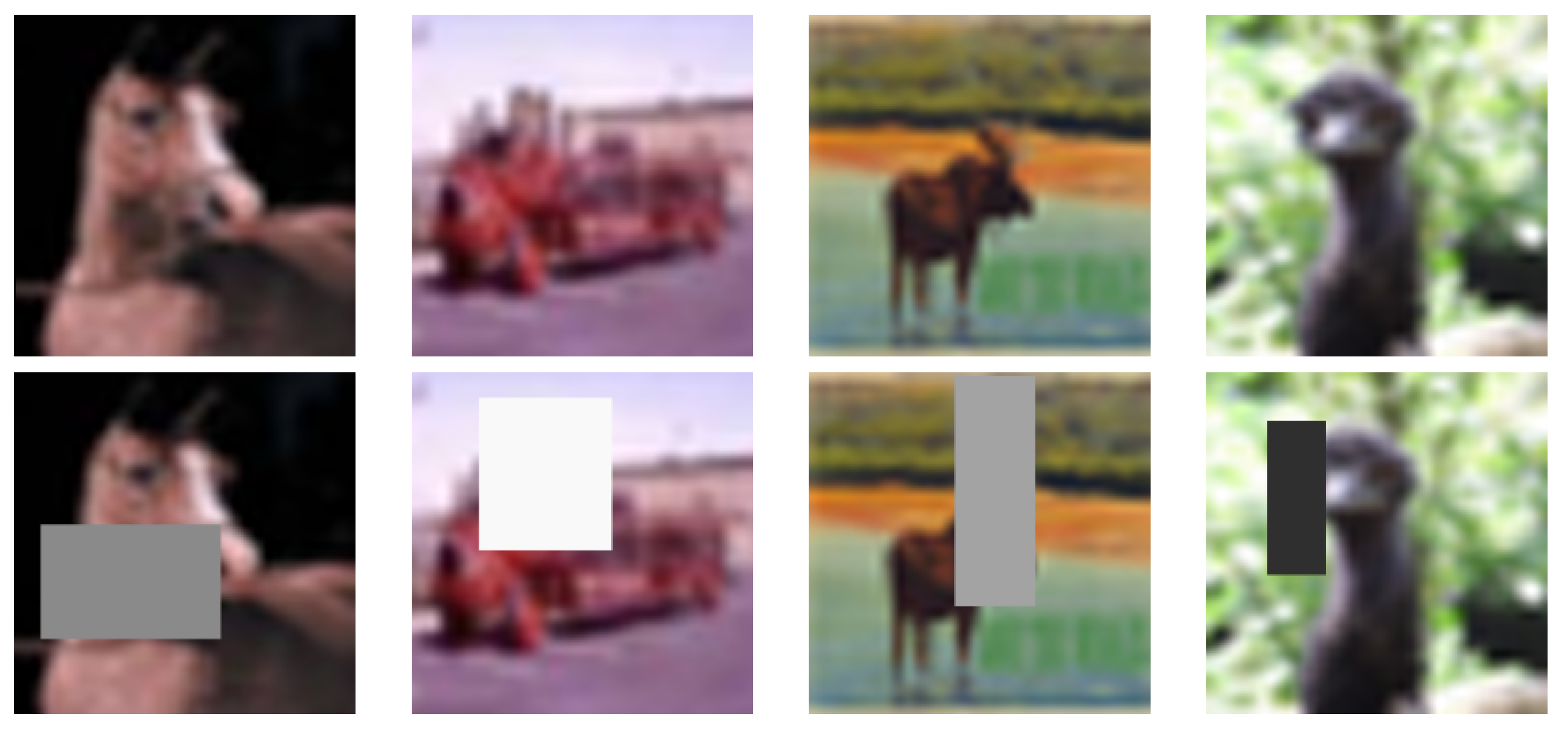
Figure 11.
Data augmentation by the random erasing technique. The first and second rows represent the given images (from CIFAR-10) and the images after random erasing, respectively.
Figure 11.
Data augmentation by the random erasing technique. The first and second rows represent the given images (from CIFAR-10) and the images after random erasing, respectively.
Figure 12.
Data augmentation by texture transfer. Content of the base image (left) is mixed with the style of the reference style image (middle) to obtain the resultant image (right).
Figure 12.
Data augmentation by texture transfer. Content of the base image (left) is mixed with the style of the reference style image (middle) to obtain the resultant image (right).
Figure 13.
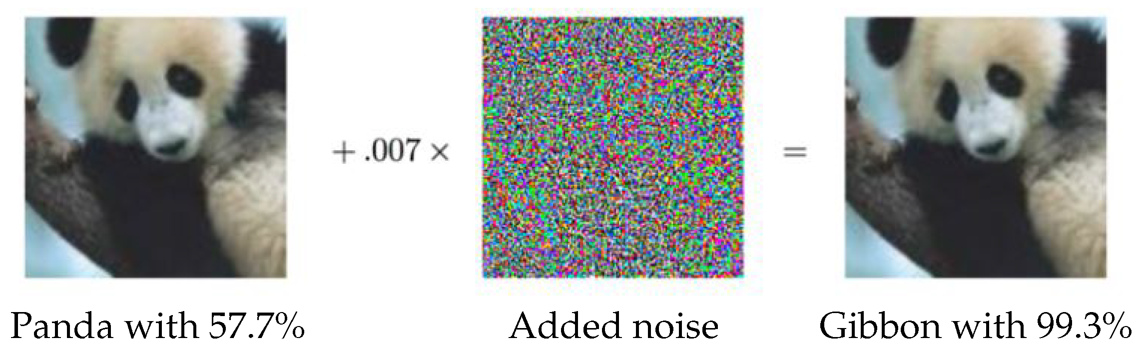
An adversarial example taken from [
61]. Even though the given image and the image after adversarial noise added look exactly the same to the human eye, the noise fools the model successfully, i.e., the model labels the two images as different classes.
Figure 13.
An adversarial example taken from [
61]. Even though the given image and the image after adversarial noise added look exactly the same to the human eye, the noise fools the model successfully, i.e., the model labels the two images as different classes.
Figure 14.
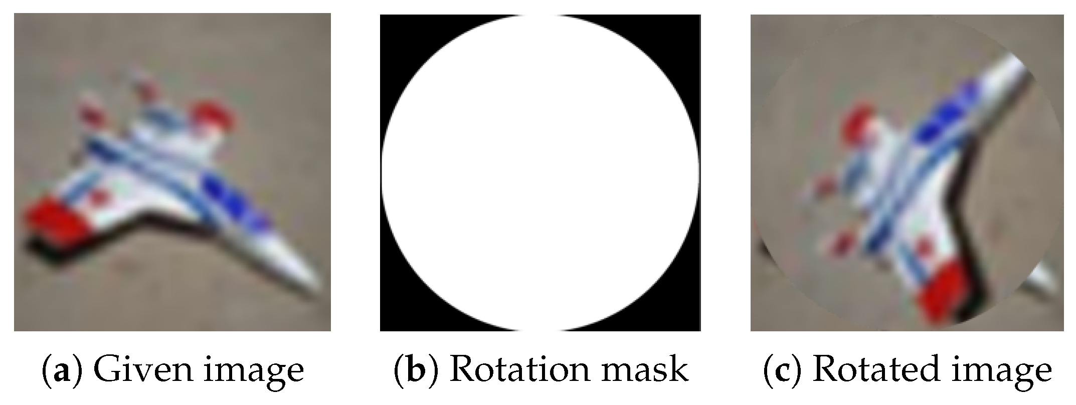
The proposed random local rotation data augmentation strategy. Symbol ⊙ represents pointwise multiplication.
Figure 14.
The proposed random local rotation data augmentation strategy. Symbol ⊙ represents pointwise multiplication.
Figure 15.
Random local rotation data augmentation technique using the largest possible circular rotation area in the image centre.
Figure 15.
Random local rotation data augmentation technique using the largest possible circular rotation area in the image centre.
Figure 16.
Data augmentation techniques evaluation by saliency map. Column 1: given images; columns 2 and 3: two types of saliency maps for TR; columns 4 and 5: two types of saliency maps for RLR. In particular, for the two types of saliency maps evaluating each data augmentation technique, the first saliency map highlights the activated area in the given image, and the second highlights the activated area using the content of the given image. The CNNs used for the test images in the first and second rows are MobileNet and ResNet50, respectively. The saliency maps created for the models, which were trained with the dataset augmented with RLR, clearly focus on the wider part of the object while for the other cases where augmentation is achieved with TR, the models focus on a smaller area of the object. The models trained with RLR output more reliable results, together with the wider focus on the target object shown in the above saliency maps, demonstrating the superior performance of RLR compared to TR.
![Jimaging 09 00046 g016]()
Figure 17.
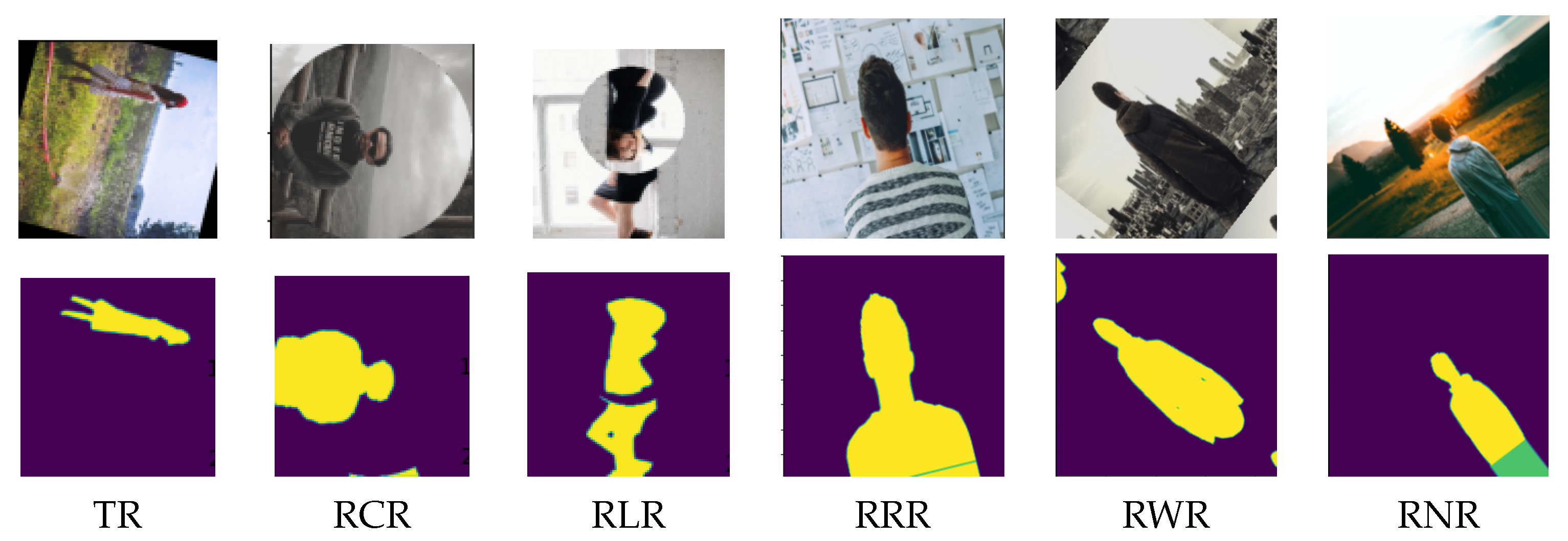
Samples of the Supervisely Person dataset by applying the RLR, TR, RCR, RRR, RWR and RNR augmentation techniques. Rows one and two are the augmented samples with their corresponding human body segmentation, respectively.
Figure 17.
Samples of the Supervisely Person dataset by applying the RLR, TR, RCR, RRR, RWR and RNR augmentation techniques. Rows one and two are the augmented samples with their corresponding human body segmentation, respectively.
Figure 18.
Samples of the Nuclei images dataset by applying the RLR, TR, RCR, RRR, RWR and RNR augmentation techniques. Rows one and two are the augmented samples with their corresponding segmentation, respectively.
Figure 18.
Samples of the Nuclei images dataset by applying the RLR, TR, RCR, RRR, RWR and RNR augmentation techniques. Rows one and two are the augmented samples with their corresponding segmentation, respectively.
Figure 19.
The effect of different rotation methods on the rotated image. The RRR and RWR expanded the central region (i.e., the black stripe) by repeating parts of it. RNR resulted in the loss of image content at the image’s periphery and the creation of artificial pixel values to fill the gap. In contrast, RLR manipulated the content of the image while preserving the information around the image’s periphery well.
Table 1.
Survey of data augmentation techniques in recent image classification works.
Table 1.
Survey of data augmentation techniques in recent image classification works.
| Papers | Dataset | Aug. Techniques | Model | Task | Findings |
|---|
| Shijie et al., 2017 [34] | CIFAR10; ImageNet (10 categories) | GAN/WGAN, flipping, cropping, shifting, PCA jittering, colour jittering, noise, rotation. | AlexNet | Image classification | Four methods (i.e., cropping, flipping, WGAN and rotation) perform generally better than other augmentation methods, and some appropriate combination methods are slightly more effective than the individuals. |
| Perez et al., 2017 [67] | A small subset of ImageNet; MNIST. | Neural augmentation, CycleGAN, GANs, cropping, rotating, and flipping. | SmallNet | Image classification | GANs do not perform better than traditional techniques. |
| Hussain et al., 2017 [68] | Digital Database for Screening Mammography (DDSM). | Flipping, cropping, noise, Gaussian filters, principal component analysis (PCA). | VGG-16 | Medical images classification | The flipping and Gaussian filter techniques are better than noise transformation. |
| Pawara et al., 2017 [69] | Folio, AgrilPlant, and the Swedish Leaf datasets | Rotation, blur, contrast, scaling, illumination, and projective transformation. | AlexNet; GoogleNet | Plant image classification | CNN models trained from scratch benefit significantly from data augmentation. |
| Inoue et al., 2018 [70] | ILSVRC2012; CIFAR-10 | SamplePairing, flipping, distorting, noise, and cropping. | GoogLeNet | Image classification | Developed a new technique known as SamplePairing. |
| Li et al., 2018 [71] | Indian Pines and Salinas datasets | Pixel-block pair, flipping, rotation, and noise. | PBP-CNN | Hyperspectral imagery classification | A threefold increase in sample size is often sufficient to reach the upper bound. |
| Frid-Adar et al., 2018 [72] | Liver lesions dataset | Translation, rotation, scaling, flipping and shearing, and GAN-based synthetic images. | Customised small CNN architecture | Medical image classification | Combining traditional data augmentation with GAN-based synthetic images improves small datasets. |
| Pham et al., 2018 [73] | Skin lesion dataset (ISBI Challenge) | Geometric augmentation and colour augmentation. | InceptionV4 | Skin cancer image classification | Skin cancer and medical image classifiers could benefit from data augmentation. |
| Motlagh et al., 2018 [74] | Tissue Micro Array; Breast Cancer Histopathological Images (BreaKHis) | Random resizing, rotating, cropping, and flipping. | ResNet50 | Breast cancer image classification | Traditional data augmentation techniques are adequate for obtaining distinct samples of various types of cancer. |
| Zheng et al., 2019 [75] | Caltech 101; Caltech 256. | Neural style transfer, rotation, and flipping. | VGG16 | Image classification | Neural style transfer can be utilised as a deep-learning data augmentation technique. |
| Ismael et al., 2020 [76] | Brain tumor dataset | Horizontal and vertical flips, rotating, shifting, zooming, shearing, and brightness alteration. | ResNet | MRI image classification
(Brain Cancer) | The effectiveness of traditional augmentation methods varied among classes. |
| Gour et al., 2020 [77] | BreaKHis dataset | Stain normalisation, image patch generation, and affine transformation. | ResHist model | Breast cancer histopathological image classification | The model performance for classifying histopathology images is better with data augmentation than with pre-trained networks. |
| Nanni et al., 2021 [78] | Virus, a bark, a portrait, and a LIGO glitches datasets | Kernel filters, colour space transforms, geometric transformations, and random erasing. | ResNet50 | Image classification | Introduced the discrete wavelet transform and the constant-Q Gbor transform as two new methods for data augmentation. |
| Anwar et al., 2021 [79] | Customised image based ECG signals | Flipping, cropping, contrast and Gamma distortion. | EfficientNet B3 | ECG images classification | In the experiment with images of ECG signal, traditional data augmentation did not improve the performance of neural networks. |
| Kandel et al., 2021 [80] | MURA dataset | Horizontal flip, vertical flip, rotation, and zooming. | VGG19; ResNet50; InceptionV3; Xception; DenseNet121 | X-ray images classification | Augmentation was found to significantly enhance classification performance. |
Table 3.
Classification accuracy comparison between the TR, RCR and RLR data augmentation techniques. CNN models, i.e., MobileNet, ResNet and InceptionV3, with the data augmentation techniques, were applied on three different CIFAR-10 subsets, with numbers of samples of 1000, 2000 and 3000, respectively. The results indicated the superior performance of the proposed RLR technique.
| Model | Subset | Baseline | RLR | TR | RCR |
|---|
| | 1000 | | | | |
| MobileNet | 2000 | | | | |
| | 3000 | | | | |
| | 1000 | | | | |
| ResNet | 2000 | | | | |
| | 3000 | | | | |
| | 1000 | | | | |
| InceptionV3 | 2000 | | | | |
| | 3000 | | | | |
Table 4.
Classification accuracy comparison between RLR and other common data augmentation techniques. CNN models, i.e., MobileNet, ResNet and InceptionV3, with the data augmentation techniques, were applied on the smallest subset of CIFAR-10 (i.e., the one with 1000 samples).
Table 4.
Classification accuracy comparison between RLR and other common data augmentation techniques. CNN models, i.e., MobileNet, ResNet and InceptionV3, with the data augmentation techniques, were applied on the smallest subset of CIFAR-10 (i.e., the one with 1000 samples).
| Model | Baseline | RLR | RNR | Flip | Shift | Zoom | Bright | RWR | RRR |
|---|
| MobileNet | | | | | | | | | |
| ResNet | | | | | | | | | |
| InceptionV3 | | | | | | | | | |
Table 5.
The architectures of the decoders of the MobileNet-based and VGG16-based auto-encoders. Conv2D and Conv2DT represent the 2D convolutional layer and the transposed 2D convolutional layer, respectively.
Table 5.
The architectures of the decoders of the MobileNet-based and VGG16-based auto-encoders. Conv2D and Conv2DT represent the 2D convolutional layer and the transposed 2D convolutional layer, respectively.
| MobileNet Decoder | VGG16 Decoder |
|---|
| Layer | Kernel | Filters | Activation | Layer | Kernel | Filters | Activation |
| | Size | Number | Function | | Size | Number | Function |
| Conv2DT | (3,3) | 1024 | Relu | Conv2DT | (3,3) | 1024 | Relu |
| Batch Normalisation | Batch Normalisation |
| Conv2D | (3,3) | 1024 | Relu | Conv2D | (3,3) | 1024 | Relu |
| Batch Normalisation | Batch Normalisation |
| Conv2DT | (3,3) | 512 | Relu | Conv2DT | (3,3) | 512 | Relu |
| Batch Normalisation | Batch Normalisation |
| Conv2D | (3,3) | 512 | Relu | Conv2D | (3,3) | 512 | Relu |
| Batch Normalisation | Batch Normalisation |
| Conv2DT | (3,3) | 256 | Relu | Conv2DT | (3,3) | 256 | Relu |
| Batch Normalisation | Batch Normalisation |
| Conv2D | (3,3) | 256 | Relu | Conv2D | (3,3) | 256 | Relu |
| Batch Normalisation | Batch Normalisation |
| Conv2DT | (3,3) | 128 | Relu | Conv2DT | (3,3) | 128 | Relu |
| Batch Normalisation | Batch Normalisation |
| Conv2D | (3,3) | 128 | Relu | Conv2D | (3,3) | 128 | Relu |
| Batch Normalisation | Batch Normalisation |
| Conv2DT | (3,3) | 64 | Relu | Conv2DT | (3,3) | 64 | Relu |
| Batch Normalisation | Batch Normalisation |
| Conv2D | (3,3) | 64 | Relu | Conv2D | (3,3) | 64 | Relu |
| Batch Normalisation | Batch Normalisation |
| Conv2DT | (3,3) | 32 | Relu | Conv2DT | (3,3) | 32 | Relu |
| Batch Normalisation | Batch Normalisation |
| Conv2D | (3,3) | 32 | Relu | Conv2D | (2,2) | 32 | Relu |
| Batch Normalisation | Batch Normalisation |
| Conv2D | (3,3) | 1 | Sigmoid | Conv2D | (3,3) | 1 | Sigmoid |
Table 6.
Segmentation accuracy comparison between different data augmentation techniques (i.e., TR, RCR, RLR, RNR, RWR and RRR). MobileNet-based and VGG16-based autoencoders were applied on the Supervisely Person dataset. The results indicated that using rotation solely to augment data might not be a good for the segmentation task in this case.
| Model | Baseline | RLR | TR | RCR | RNR | RWR | RRR |
|---|
| MobileNet | | | | | | | |
| VGG16 | | | | | | | |
Table 7.
Segmentation accuracy comparison between different data augmentation techniques (i.e., TR, RCR, RLR, RNR, RWR and RRR). MobileNet-based and VGG16-based autoencoders were applied on the Nuclei images dataset. The results indicated that using rotation to augment data could enhance the segmentation performance in this case.
| Model | Baseline | RLR | TR | RCR | RNR | RWR | RRR |
|---|
| MobileNet | | | | | | | |
| VGG16 | | | | | | | |


