
Age Assessment through Root Lengths of Mandibular Second and Third Permanent Molars Using Machine Learning and Artificial Neural Networks
 ,
,  ,
,
Abstract
:1. Introduction
2. Materials and Methods
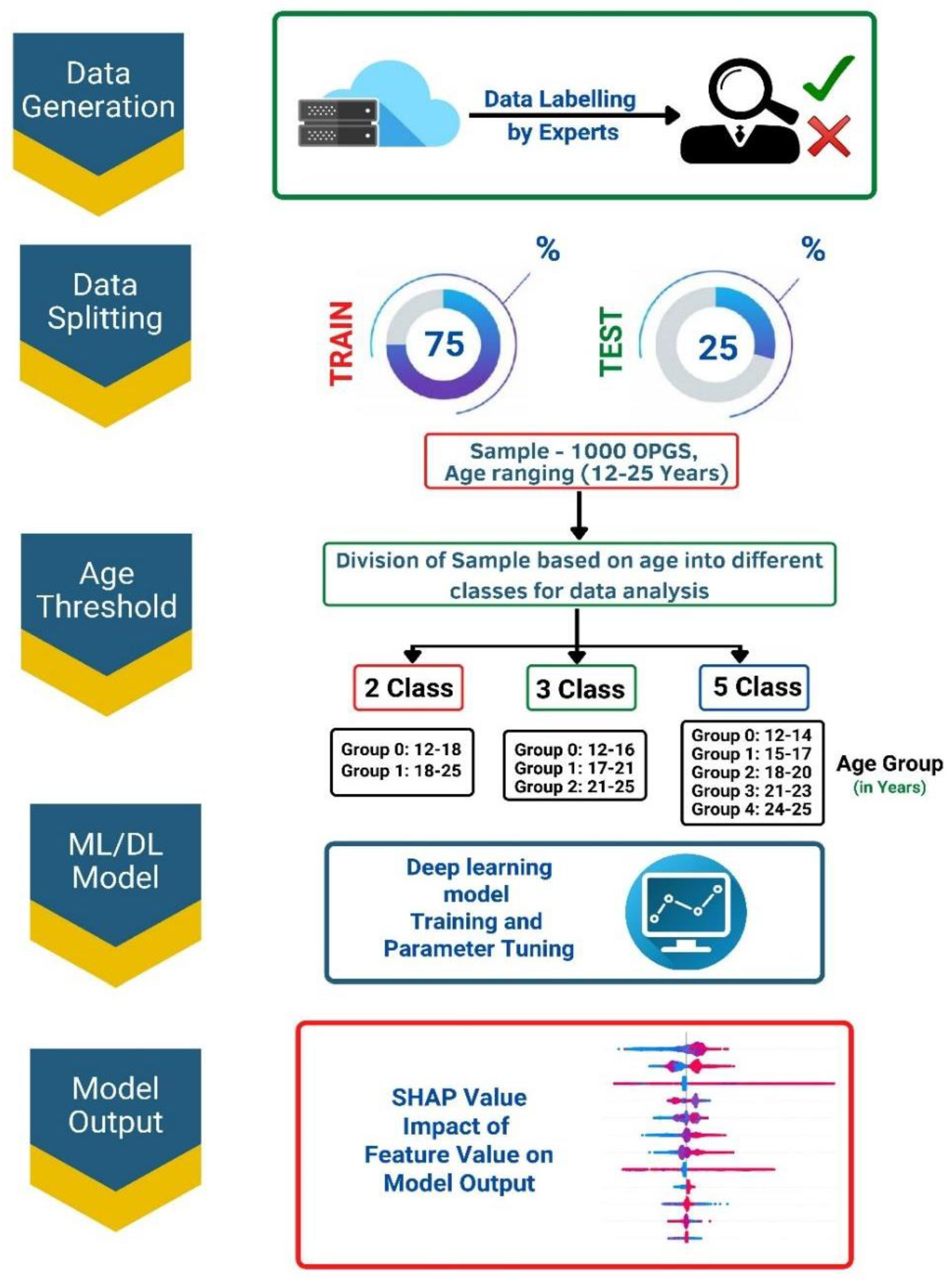
2.1. Study Design
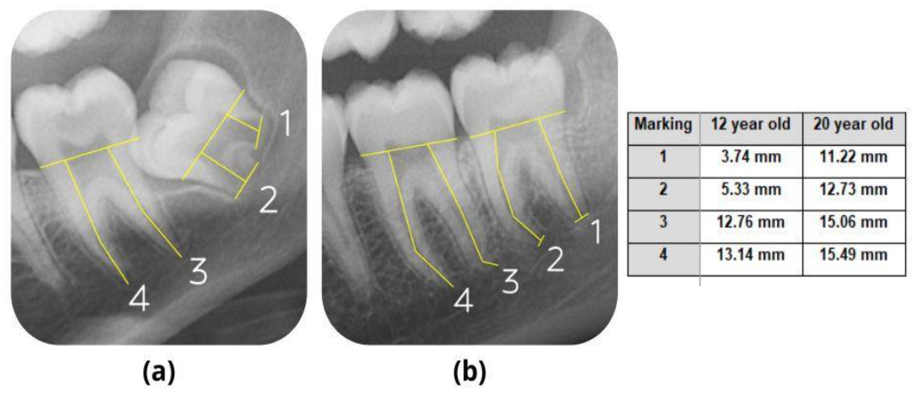
2.2. Measurements
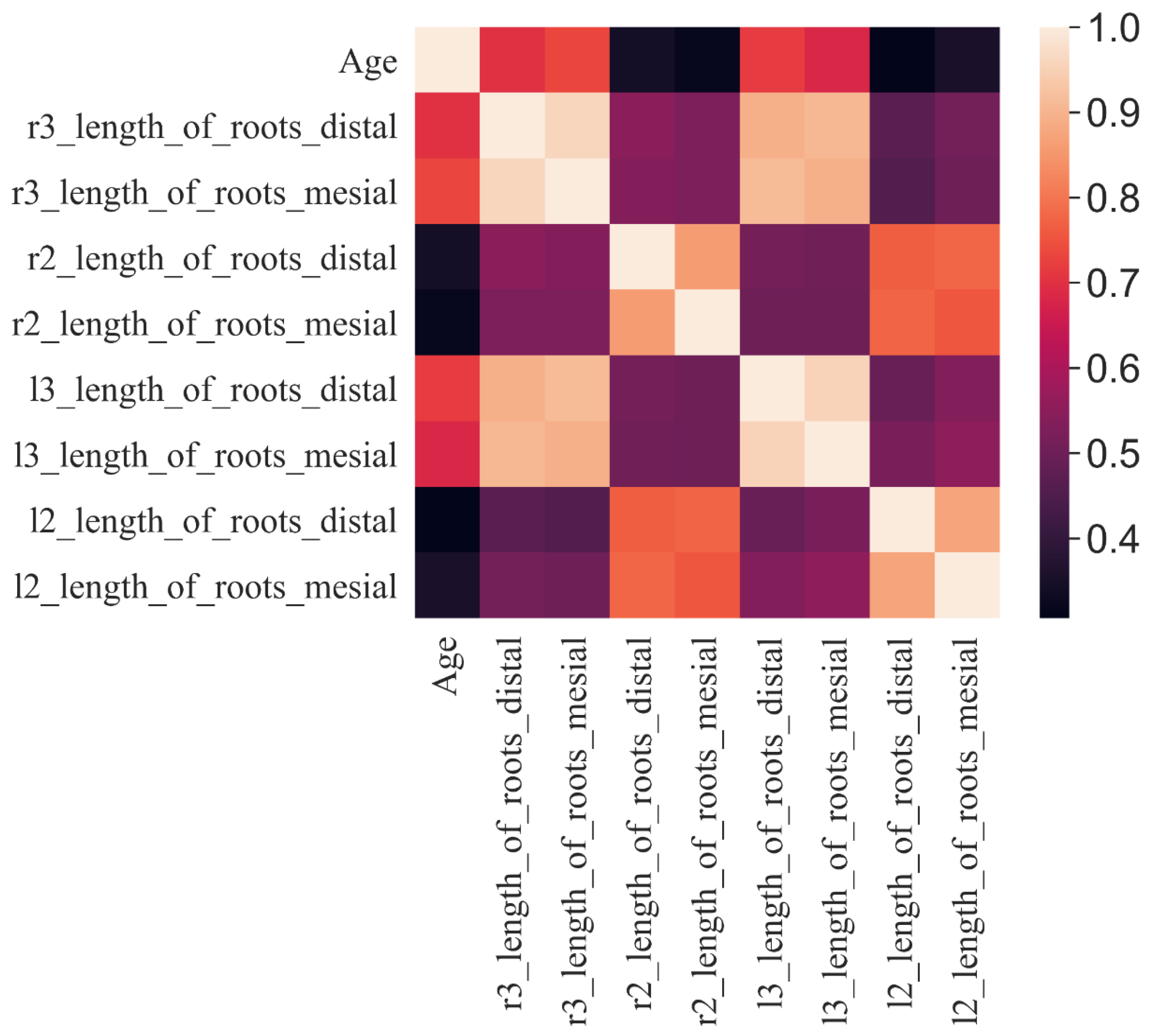
2.3. Data Processing
2.4. Computational Techniques
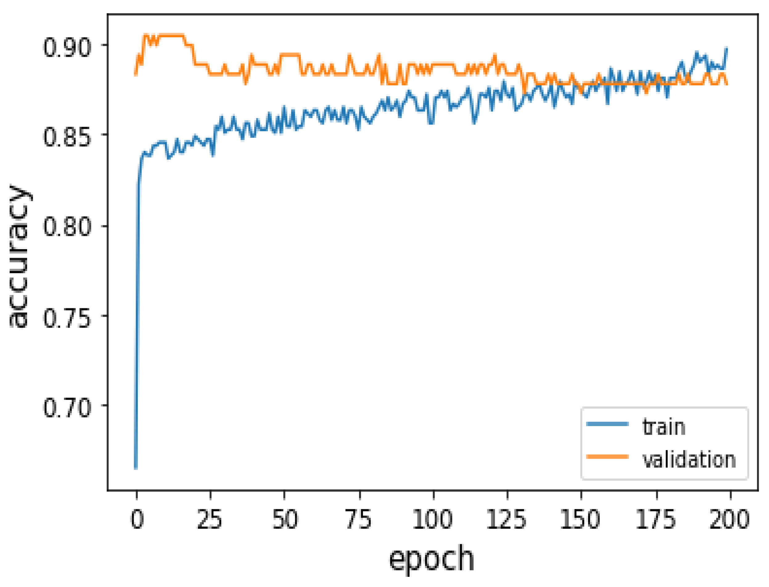
2.5. Performance Measurement
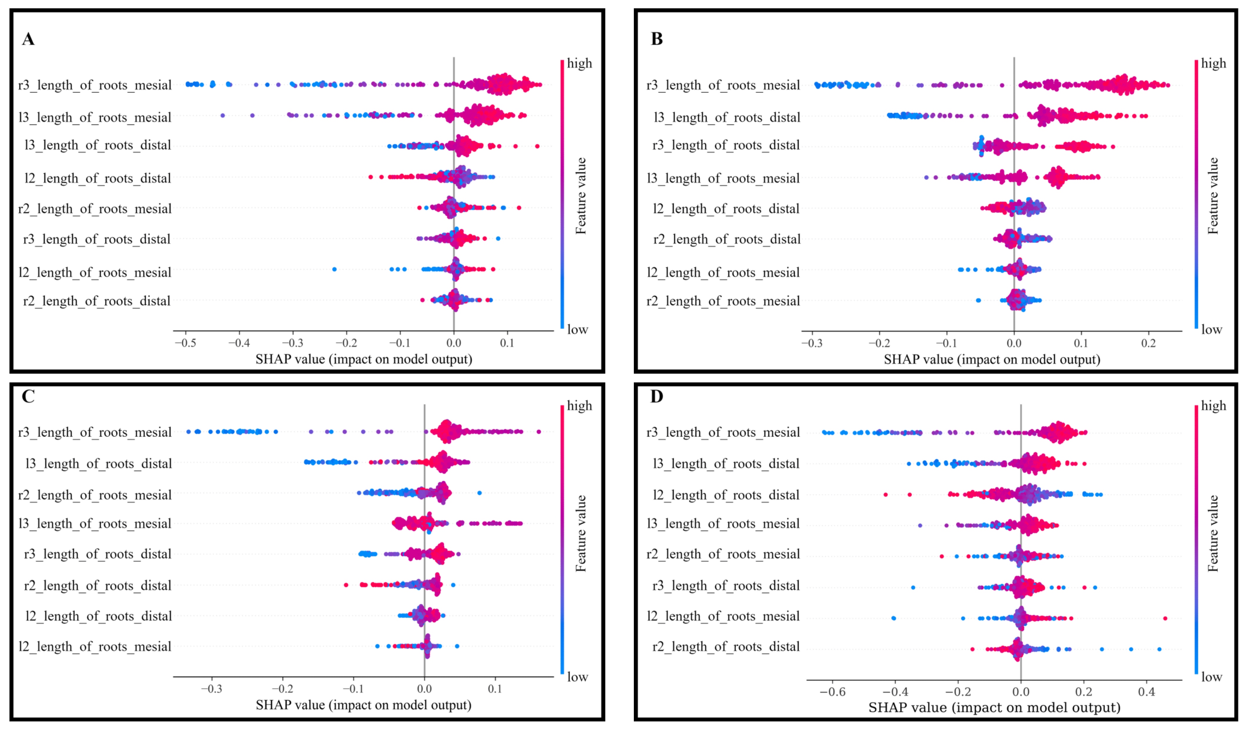
2.6. Feature Importance
3. Results
4. Regression
5. Discussion
6. Conclusions
Author Contributions
Funding
Institutional Review Board Statement
Informed Consent Statement
Data Availability Statement
Acknowledgments
Conflicts of Interest
References
- Kurniawan, A.; Chusida, A.; Atika, N.; Gianosa, T.K.; Solikhin, M.D.; Margaretha, M.S.; Utomo, H.; Marini, M.I.; Rizky, B.N.; Prakoeswa, B.F.W.R.; et al. The Applicable Dental Age Estimation Methods for Children and Adolescents in Indonesia. Int. J. Dent. 2022, 2022, 6761476. [Google Scholar] [CrossRef]
- Lossois, M.; Baccino, E. Forensic age estimation in migrants: Where do we stand? WIREs Forensic Sci. 2020, 3, e1408. [Google Scholar] [CrossRef]
- Manjrekar, S.; Deshpande, S.; Katge, F.; Jain, R.; Ghorpade, T. Age Estimation in Children by the Measurement of Open Apices in Teeth: A Study in the Western Indian Population. Int. J. Dent. 2022, 2022, 9513501. [Google Scholar] [CrossRef] [PubMed]
- Swami, D.; Mishra, V.K.; Bahal, L.; Rao, C.M. Age estimation from eruption of temporary teeth in Himachal Pradesh. J. Forensic. Med. Toxicol. 1992, 9, 3–7. [Google Scholar]
- Uzuner, F.D.; Kaygısız, E.; Darendeliler, N. Defining Dental Age for Chronological Age Determination. Post Mortem Exam Autops. 2018, 6, 77–104. [Google Scholar] [CrossRef]
- Panchbhai, A. Dental radiographic indicators, a key to age estimation. Dentomaxillofacial Radiol. 2011, 40, 199–212. [Google Scholar] [CrossRef]
- Singh, C.; Singal, K. Teeth as a tool for age estimation: A mini review. Age 2017, 11, 4–56. [Google Scholar] [CrossRef]
- AlQahtani, S. Dental Age Assessment. Forensic Odontology: An Essential Guide; John Wiley & Sons: Hoboken, NJ, USA, 2014; pp. 137–166. [Google Scholar]
- Kvaal, S.I.; Kolltveit, K.M.; Thomsen, I.O.; Solheim, T. Age estimation of adults from dental radiographs. Forensic Sci. Int. 1995, 74, 175–185. [Google Scholar] [CrossRef]
- Narnbiar, P. Age estimation using third molar development. Malaysian J. Pathol. 1995, 17, 31–34. [Google Scholar]
- Guo, Y.-C.; Chu, G.; Olze, A.; Schmidt, S.; Schulz, R.; Ottow, C.; Pfeiffer, H.; Chen, T.; Schmeling, A. Age estimation of Chinese children based on second molar maturity. Int. J. Leg. Med. 2017, 132, 807–813. [Google Scholar] [CrossRef]
- Fins, P.; Pereira, M.L.; Afonso, A.; Pérez–Mongiovi, D.; Caldas, I.M. Chronology of mineralization of the permanent mandibular second molar teeth and forensic age estimation. Forensic Sci. Med. Pathol. 2017, 13, 272–277. [Google Scholar] [CrossRef] [PubMed]
- Schwendicke, F.; Samek, W.; Krois, J. Artificial Intelligence in Dentistry: Chances and Challenges. J. Dent. Res. 2020, 99, 769–774. [Google Scholar] [CrossRef] [PubMed]
- Sweet, D. Why a dentist for identification? Dent. Clin. N. Am. 2001, 45, 237–251. [Google Scholar] [CrossRef] [PubMed]
- Jambunath, U.; Govindraju, P.; Balaji, P.; Poornima, C.; Latha, S.F. Sex determination by using mandibular ramus and gonial angle—A preliminary comparative study. Int. J. Contem. Med. Res. 2016, 3, 3278–3280. [Google Scholar]
- Acharya, A.B.; Prabhu, S.; Muddapur, M.V. Odontometric sex assessment from logistic regression analysis. Int. J. Leg. Med. 2010, 125, 199–204. [Google Scholar] [CrossRef]
- Angadi, P.V.; Hemani, S.; Prabhu, S.; Acharya, A.B. Analyses of odontometric sexual dimorphism and sex assessment accuracy on a large sample. J. Forensic Leg. Med. 2013, 20, 673–677. [Google Scholar] [CrossRef]
- Patil, V.; Vineetha, R.; Vatsa, S.; Shetty, D.K.; Raju, A.; Naik, N.; Malarout, N. Artificial neural network for gender determination using mandibular morphometric parameters: A comparative retrospective study. Cogent Eng. 2020, 7, 1723783. [Google Scholar] [CrossRef]
- Santosh, K.C.; Pradeep, N.; Goel, V.; Ranjan, R.; Pandey, E.; Shukla, P.K.; Nuagah, S.J. Machine Learning Techniques for Human Age and Gender Identification Based on Teeth X–Ray Images. J. Health Eng. 2022, 2022, 8302674. [Google Scholar] [CrossRef] [PubMed]
- Kim, S.; Lee, Y.-H.; Noh, Y.-K.; Park, F.C.; Auh, Q.-S. Age–group determination of living individuals using first molar images based on artificial intelligence. Sci. Rep. 2021, 11, 1073. [Google Scholar] [CrossRef]
- Kahaki, S.M.M.; Nordin, J.; Ahmad, N.S.; Arzoky, M.; Ismail, W. Deep convolutional neural network designed for age assessment based on orthopantomography data. Neural Comput. Appl. 2019, 32, 9357–9368. [Google Scholar] [CrossRef]
- Vishwanathan, S.V.; Smola, A.; Murty, N. SSVM: A simple SVM algorithm. In Proceedings of the 2002 International Joint Conference on Neural Networks, Honolulu, HI, USA, 12–17 May 2002; Volume 3, pp. 2393–2398. [Google Scholar]
- Biau, G. Analysis of a random forests model. J. Mach. Learn. Res. 2012, 13, 1063–1095. [Google Scholar]
- Nusinovici, S.; Tham, Y.C.; Yan, M.Y.C.; Ting, D.S.W.; Li, J.; Sabanayagam, C.; Wong, T.Y.; Cheng, C.-Y. Logistic regression was as good as machine learning for predicting major chronic diseases. J. Clin. Epidemiol. 2020, 122, 56–69. [Google Scholar] [CrossRef] [PubMed]
- Minderer, M.; Djolonga, J.; Romijnders, R.; Hubis, F.; Zhai, X.; Houlsby, N.; Tran, D.; Lucic, M. Revisiting the calibration of modern neural networks. Adv. Neural Inf. Process. Syst. 2021, 34, 15682–15694. [Google Scholar]
- Dong, S.; Wang, P.; Abbas, K. A survey on deep learning and its applications. Comput. Sci. Rev. 2021, 40, 100379. [Google Scholar] [CrossRef]
- Janiesch, C.; Zschech, P.; Heinrich, K. Machine learning and deep learning. Electron. Mark. 2021, 31, 685–695. [Google Scholar] [CrossRef]
- Bartlett, P.L.; Montanari, A.; Rakhlin, A. Deep learning: A statistical viewpoint. Acta Numer. 2021, 30, 87–201. [Google Scholar] [CrossRef]
- Kerrigan, G.; Smyth, P.; Steyvers, M. Combining human predictions with model probabilities via confusion matrices and calibration. Adv. Neural Inf. Process. Syst. 2021, 34, 4421–4434. [Google Scholar]
- Naik, N.; Hameed, B.M.Z.; Shetty, D.K.; Swain, D.; Shah, M.; Paul, R.; Aggarwal, K.; Ibrahim, S.; Patil, V.; Smriti, K.; et al. Legal and Ethical Consideration in Artificial Intelligence in Healthcare: Who Takes Responsibility? Front. Surg. 2022, 9, 862322. [Google Scholar] [CrossRef]
- Naik, N.; Rallapalli, Y.; Krishna, M.; Vellara, A.S.; Shetty, D.K.; Patil, V.; Hameed, B.Z.; Paul, R.; Prabhu, N.; Rai, B.P.; et al. Demystifying the Advancements of Big Data Analytics in Medical Diagnosis: An Overview. Eng. Sci. 2022, 19, 42–58. [Google Scholar] [CrossRef]
- Hameed, M.M.; AlOmar, M.K.; Khaleel, F.; Al–Ansari, N. An Extra Tree Regression Model for Discharge Coefficient Prediction: Novel, Practical Applications in the Hydraulic Sector and Future Research Directions. Math. Probl. Eng. 2021, 2021, 7001710. [Google Scholar] [CrossRef]
- Memon, N.; Patel, S.B.; Patel, D.P. Comparative analysis of artificial neural network and XGBoost algorithm for PolSAR image classification. In Proceedings of the International Conference on Pattern Recognition and Machine Intelligence 2019, Tezpur, India, 17–20 December 2019; Springer: Berlin/Heidelberg, Germany; pp. 452–460. [Google Scholar]
- Rapp, M. BOOMER—An algorithm for learning gradient boosted multi–label classification rules. Softw. Impacts 2021, 10, 100137. [Google Scholar] [CrossRef]
- Sugiharti, E.; Arifudin, R.; Wiyanti, D.T.; Susilo, A.B. Integration of convolutional neural network and extreme gradient boosting for breast cancer detection. Bull. Electr. Eng. Inform. 2022, 11, 803–813. [Google Scholar] [CrossRef]
- Antwarg, L.; Miller, R.M.; Shapira, B.; Rokach, L. Explaining anomalies detected by autoencoders using Shapley Additive Explanations. Expert Syst. Appl. 2021, 186, 115736. [Google Scholar] [CrossRef]
- Chadaga, K.; Prabhu, S.; Umakanth, S.; Bhat, K.; Sampathila, N.; Chadaga, R. COVID–19 Mortality Prediction among Patients using Epidemiological parameters: An Ensemble Machine Learning Approach. Eng. Sci. 2021, 16, 221–233. [Google Scholar] [CrossRef]
- Maber, M.; Liversidge, H.; Hector, M. Accuracy of age estimation of radiographic methods using developing teeth. Forensic Sci. Int. 2006, 159, S68–S73. [Google Scholar] [CrossRef]
- Logan, W.H.; Kronfeld, R. Development of the human jaws and surrounding structures from birth to the age of fifteen years. J. Am. Dent. Assoc. 1933, 20, 379–428. [Google Scholar] [CrossRef]
- Boonpitaksathit, T.; Hunt, N.; Roberts, G.J.; Petrie, A.; Lucas, V.S. Dental age assessment of adolescents and emerging adults in United Kingdom Caucasians using censored data for stage H of third molar roots. Eur. J. Orthod. 2010, 33, 503–508. [Google Scholar] [CrossRef]
- Gunst, K.; Mesotten, K.; Carbonez, A.; Willems, G. Third molar root development in relation to chronological age: A large sample sized retrospective study. Forensic Sci. Int. 2003, 136, 52–57. [Google Scholar] [CrossRef]
- Mohammed, R.B. Accuracy of Four Dental Age Estimation Methods in Southern Indian Children. J. Clin. Diagn. Res. 2015, 9, HC01–HC08. [Google Scholar] [CrossRef]
- Willmot, S.E.; Hector, M.P.; Liversidge, H.M. Accuracy of estimating age from eruption levels of mandibular teeth. Dent. Anthr. J. 2018, 26, 56–62. [Google Scholar] [CrossRef]
- Mesotten, K.; Gunst, K.; Carbonez, A.; Willems, G. Dental age estimation and third molars: A preliminary study. Forensic Sci. Int. 2002, 129, 110–115. [Google Scholar] [CrossRef] [PubMed]


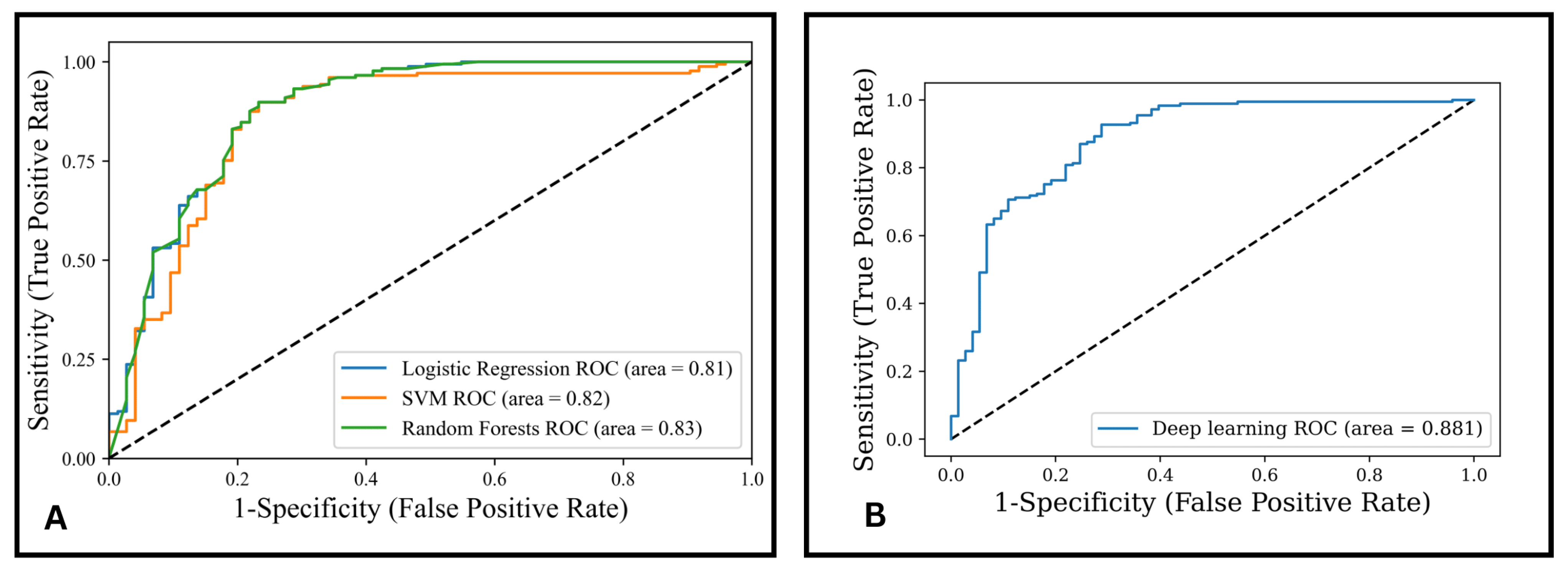
| Class Division | Classifier | Accuracy | AUC | Recall | Precision |
|---|---|---|---|---|---|
| 2–Class | SVM | 86.8 | 0.82 | 0.93 | 0.89 |
| RF | 86.0 | 0.83 | 0.90 | 0.90 | |
| Logistic Regression | 84.8 | 0.81 | 0.90 | 0.88 | |
| 3–Class | SVM | 66.0 | – | 0.58 | 0.50 |
| RF | 60.0 | 0.69 | 0.67 | ||
| Logistic Regression | 60.4 | 0.69 | 0.62 | ||
| 5–Class | SVM | 44.0 | – | 0.50 | 0.50 |
| RF | 42.4 | 0.42 | 0.43 | ||
| Logistic Regression | 40.4 | 0.51 | 0.46 |
| Class Division | Classifier | Accuracy | AUC | Recall | Precision |
|---|---|---|---|---|---|
| 2–Class | SVM | 86.4 | 0.82 | 0.93 | 0.88 |
| RF | 85.6 | 0.80 | 0.93 | 0.87 | |
| Logistic Regression | 84.0 | 0.79 | 0.90 | 0.87 | |
| 3–Class | SVM | 66.0 | – | 0.58 | 0.50 |
| RF | 60.0 | 0.60 | 0.65 | ||
| Logistic Regression | 60.4 | 0.67 | 0.62 | ||
| 5–Class | SVM | 42.8 | – | 0.50 | 0.49 |
| RF | 47.6 | 0.47 | 0.44 | ||
| Logistic Regression | 40.4 | 0.47 | 0.44 |
| Class Division | Model | Accuracy | AUC | Recall | Precision |
|---|---|---|---|---|---|
| 2–Class | Classification using Deep Learning | 87.2 | 0.88 | 0.96 | 0.87 |
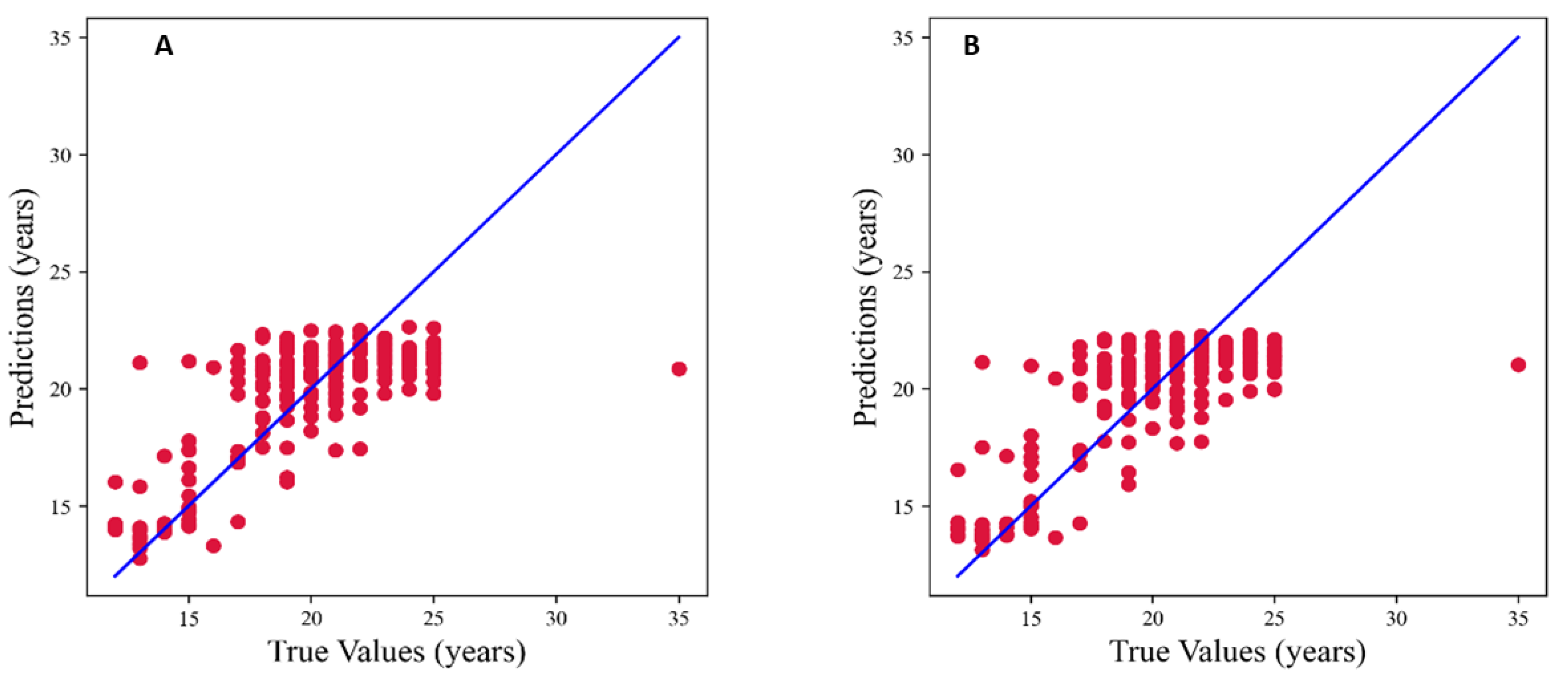
| Regressor | R Square Value | MAE | RMSE |
|---|---|---|---|
| Random Forest Regressor | 0.58 | 1.83 | 2.40 |
| Extra Tree Regressor | 0.58 | 1.81 | 2.38 |
| XGBoost Regressor | 0.57 | 1.83 | 2.41 |
| Gradient Boosting Regressor | 0.57 | 1.85 | 2.41 |
Disclaimer/Publisher’s Note: The statements, opinions and data contained in all publications are solely those of the individual author(s) and contributor(s) and not of MDPI and/or the editor(s). MDPI and/or the editor(s) disclaim responsibility for any injury to people or property resulting from any ideas, methods, instructions or products referred to in the content. |
© 2023 by the authors. Licensee MDPI, Basel, Switzerland. This article is an open access article distributed under the terms and conditions of the Creative Commons Attribution (CC BY) license (https://creativecommons.org/licenses/by/4.0/).
Share and Cite
Patil, V.; Saxena, J.; Vineetha, R.; Paul, R.; Shetty, D.K.; Sharma, S.; Smriti, K.; Singhal, D.K.; Naik, N. Age Assessment through Root Lengths of Mandibular Second and Third Permanent Molars Using Machine Learning and Artificial Neural Networks. J. Imaging 2023, 9, 33. https://doi.org/10.3390/jimaging9020033
Patil V, Saxena J, Vineetha R, Paul R, Shetty DK, Sharma S, Smriti K, Singhal DK, Naik N. Age Assessment through Root Lengths of Mandibular Second and Third Permanent Molars Using Machine Learning and Artificial Neural Networks. Journal of Imaging. 2023; 9(2):33. https://doi.org/10.3390/jimaging9020033
Chicago/Turabian StylePatil, Vathsala, Janhavi Saxena, Ravindranath Vineetha, Rahul Paul, Dasharathraj K. Shetty, Sonali Sharma, Komal Smriti, Deepak Kumar Singhal, and Nithesh Naik. 2023. "Age Assessment through Root Lengths of Mandibular Second and Third Permanent Molars Using Machine Learning and Artificial Neural Networks" Journal of Imaging 9, no. 2: 33. https://doi.org/10.3390/jimaging9020033