
CNN-Based Classification for Highly Similar Vehicle Model Using Multi-Task Learning

Abstract
:1. Introduction
- Modifications of the CNN architecture by adding multi-task learning have increased the efficiency of the classification because it can provide two types of output (one for vehicle make and one for vehicle model) in one recognition cycle;
- Investigation of multiple CNN base architectures to perform multi-task learning for two tasks (vehicle brand and vehicle model classification) on highly similar vehicles has resulted in improved performance for all tasks across all CNN base architectures;
- Evaluation of the proposed method employing a dataset of images captured by a dashboard camera has provided a new and unique perspective in comparison to other existing car datasets.
2. Related Works
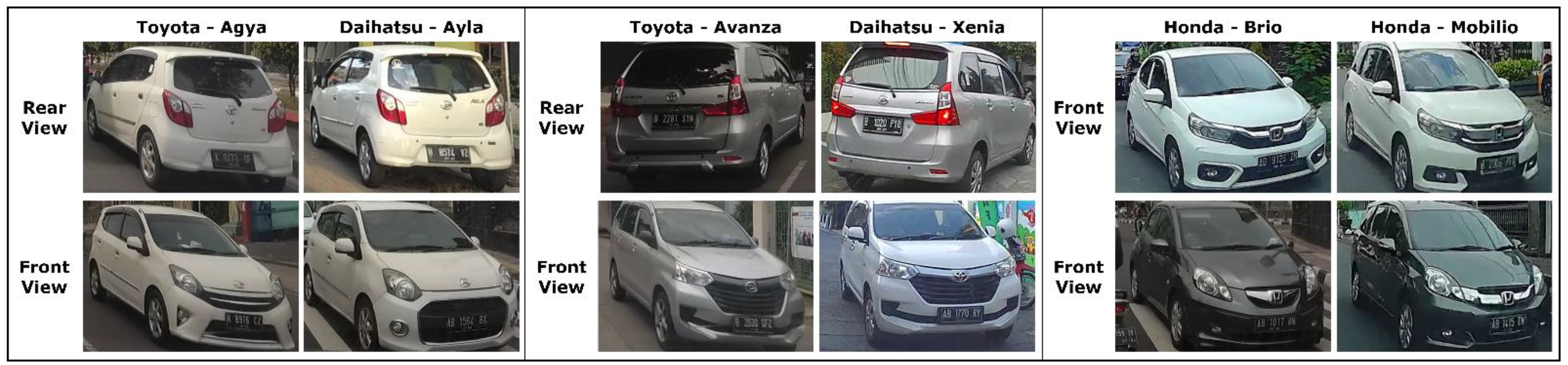
3. Dataset
InaV-Dash Dataset
4. Proposed Method
4.1. Single-Task and Multi-Task Learning
4.2. Convolutional Neural Network
4.3. Proposed Multi-Task Convolutional Neural Network
4.3.1. Convolutional Layer
4.3.2. Max-Pool Layer
4.3.3. Global Average Pooling Layer
4.3.4. Dense Layer
4.3.5. Dropout Layer
4.3.6. Activation Functions
4.3.7. Loss Function
4.4. Performance Evaluation Method
5. Results and Discussion
5.1. Experimental Setup
5.2. Experimental Results on Single-Task CNN
5.3. Experimental Results on Multi-Task CNN
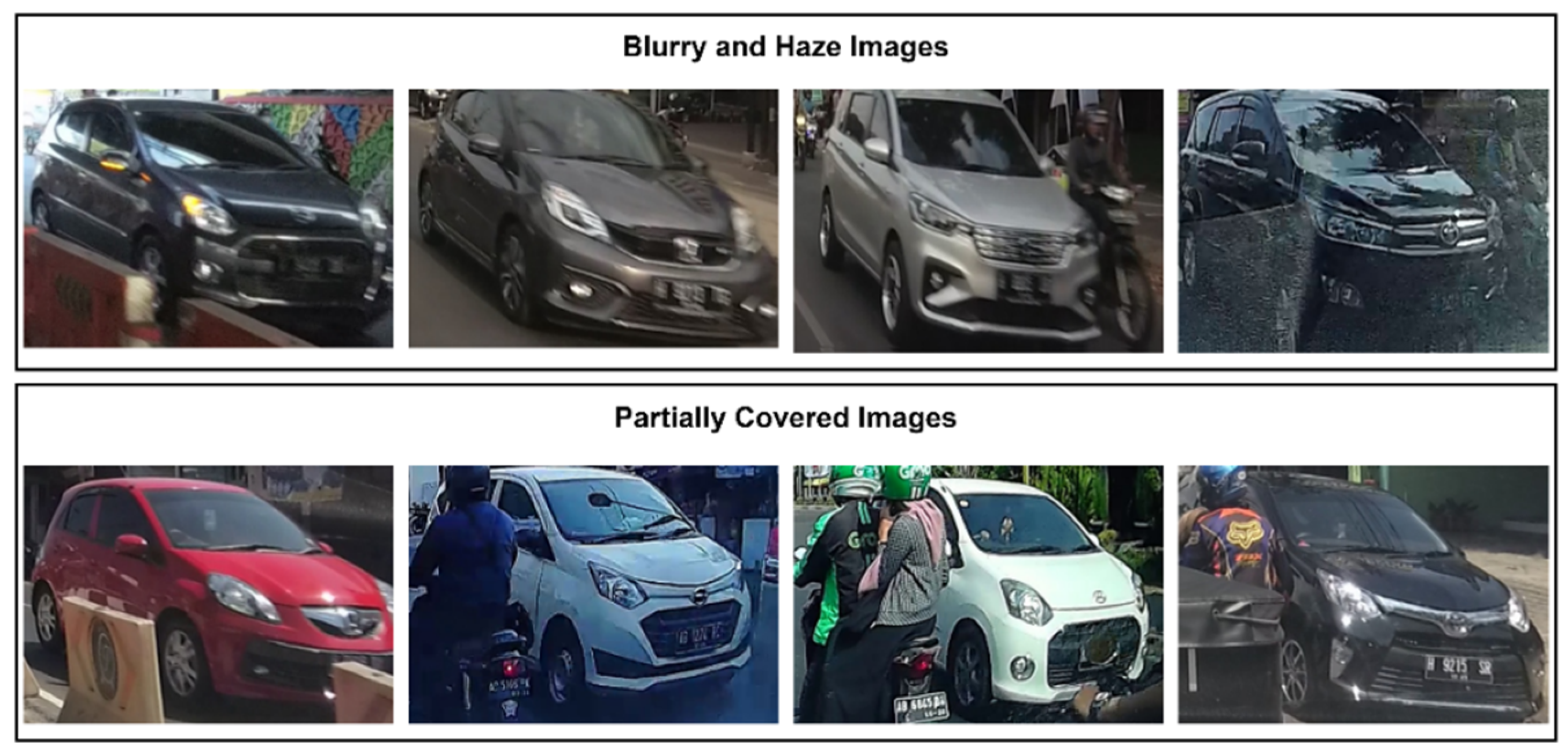
6. Limitations
7. Conclusions
Author Contributions
Funding
Institutional Review Board Statement
Informed Consent Statement
Data Availability Statement
Conflicts of Interest
References
- Akinyelu, A.A.; Zaccagna, F.; Grist, J.T.; Castelli, M.; Rundo, L. Brain Tumor Diagnosis Using Machine Learning, Convolutional Neural Networks, Capsule Neural Networks and Vision Transformers, Applied to MRI: A Survey. J. Imaging 2022, 8, 205. [Google Scholar] [CrossRef] [PubMed]
- Ahmad, S.F.; Rahmat, M.K.; Mubarik, M.S.; Alam, M.M.; Hyder, S.I. Artificial Intelligence and Its Role in Education. Sustainability 2021, 13, 12902. [Google Scholar] [CrossRef]
- Aligholi, S.; Khajavi, R.; Khandelwal, M.; Armaghani, D.J. Mineral Texture Identification Using Local Binary Patterns Equipped with a Classification and Recognition Updating System (CARUS). Sustainability 2022, 14, 11291. [Google Scholar] [CrossRef]
- Abduljabbar, R.; Dia, H.; Liyanage, S.; Bagloee, S.A. Applications of Artificial Intelligence in Transport: An Overview. Sustainability 2019, 11, 189. [Google Scholar] [CrossRef] [Green Version]
- Murali, A.; Nair, B.B.; Rao, S.N. Comparative Study of Different CNNs for Vehicle Classification. In Proceedings of the 2018 IEEE International Conference on Computational Intelligence and Computing Research (ICCIC), Madurai, India, 13–15 December 2018. [Google Scholar]
- Abbas, A.F.; Sheikh, U.U.; Mohd, M.N.H. Recognition of vehicle make and model in low light conditions. Bull. Electr. Eng. Inform. 2020, 9, 550–557. [Google Scholar] [CrossRef]
- Leotta, M.J.; Mundy, J.L. Vehicle Surveillance with a Generic, Adaptive, 3D Vehicle Model. IEEE Trans. Pattern Anal. Mach. Intell. 2011, 33, 1457–1469. [Google Scholar] [CrossRef] [PubMed]
- Satar, B.; Dirik, A.E. Deep Learning Based Vehicle Make-Model Classification. In Proceedings of the 27th International Conference on Artificial Neural Networks, Rhodes, Greece, 4–7 October 2018. [Google Scholar]
- Ghassemi, S.; Fiandrotti, A.; Caimotti, E.; Francini, G.; Magli, E. Vehicle joint make and model recognition with multiscale attention windows. Signal Process. Image Commun. 2019, 72, 69–79. [Google Scholar] [CrossRef]
- Soon, F.C.; Khaw, H.Y.; Chuah, J.H.; Kanesan, J. PCANet-Based Convolutional Neural Network Architecture for a Vehicle Model Recognition System. IEEE Trans. Intell. Transp. Syst. 2019, 20, 749–759. [Google Scholar] [CrossRef]
- Sochor, J.; Špaňhel, J.; Herout, A. BoxCars: Improving Fine-Grained Recognition of Vehicles Using 3-D Bounding Boxes in Traffic Surveillance. IEEE Trans. Intell. Transp. Syst. 2019, 20, 97–108. [Google Scholar] [CrossRef] [Green Version]
- Manzoor, M.A.; Morgan, Y. Vehicle Make and Model classification system using bag of SIFT features. In Proceedings of the 2017 IEEE 7th Annual Computing and Communication Workshop and Conference (CCWC), Las Vegas, NV, USA, 9–11 January 2017. [Google Scholar]
- Al-Maadeed, S.; Boubezari, R.; Kunhoth, S.; Bouridane, A. Robust feature point detectors for car make recognition. Comput. Ind. 2018, 100, 129–136. [Google Scholar] [CrossRef]
- Manzoor, M.A.; Morgan, Y. Vehicle make and model recognition using random forest classification for intelligent transportation systems. In Proceedings of the 2018 IEEE 8th Annual Computing and Communication Workshop and Conference (CCWC), Las Vegas, NV, USA, 8–10 January 2018. [Google Scholar]
- Yang, J.; Chen, Z.; Zhang, J.; Zhang, C.; Zhou, Q.; Yang, J. HOG and SVM algorithm based on vehicle model recognition. In Proceedings of the Eleventh International Symposium on Multispectral Image Processing and Pattern Recognition (MIPPR2019), Wuhan, China, 2–3 November 2019. [Google Scholar]
- Sotheeswaran, S.; Ramanan, A. A Coarse-to-Fine Strategy for Vehicle Logo Recognition from Frontal-View Car Images. Pattern Recognit. Image Anal. 2018, 28, 142–154. [Google Scholar] [CrossRef]
- Manzoor, M.A.; Morgan, Y.; Bais, A. Real-Time Vehicle Make and Model Recognition System. Mach. Learn. Knowl. Extr. 2019, 1, 611–629. [Google Scholar] [CrossRef] [Green Version]
- Zulkeflie, S.A.; Fammy, F.A.; Ibrahim, Z.; Sabri, N. Evaluation of basic convolutional neural network, alexnet and bag of features for indoor object recognition. Int. J. Mach. Learn. Comput. 2019, 9, 801–806. [Google Scholar] [CrossRef]
- Hsieh, J.; Chen, L.; Chen, D. Symmetrical SURF and Its Applications to Vehicle Detection and Vehicle Make and Model Recognition. IEEE Trans. Intell. Transp. Syst. 2014, 15, 6–20. [Google Scholar] [CrossRef]
- Boukerche, A.; Ma, X. A Novel Smart Lightweight Visual Attention Model for Fine-Grained Vehicle Recognition. IEEE Trans. Intell. Transp. Syst. 2021, 28, 1–17. [Google Scholar] [CrossRef]
- Siddiqui, A.J.; Boukerche, A. A Novel Lightweight Defense Method Against Adversarial Patches-Based Attacks on Automated Vehicle Make and Model Recognition Systems. J. Netw. Syst. Manag. 2021, 29, 41. [Google Scholar] [CrossRef]
- Ma, X.; Boukerche, A. An AI-based Visual Attention Model for Vehicle Make and Model Recognition. In Proceedings of the 2020 IEEE Symposium on Computers and Communications (ISCC), Rennes, France, 7–10 July 2020. [Google Scholar]
- Naseer, S.; Shah, S.M.A.; Aziz, S.; Khan, M.U.; Iqtidar, K. Vehicle Make and Model Recognition using Deep Transfer Learning and Support Vector Machines. In Proceedings of the 2020 IEEE 23rd International Multitopic Conference (INMIC), Bahawalpur, Pakistan, 5–7 November 2020. [Google Scholar]
- Liu, D.; Wang, Y. Monza: Image Classification of Vehicle Make and Model Using Convolutional Neural Networks and Transfer Learning; Stanford University: Stanford, CA, USA, 2017. [Google Scholar]
- Balci, B.; Elihos, A.; Turan, M.; Alkan, B.; Artan, Y. Front-View Vehicle Make and Model Recognition on Night-Time NIR Camera Images. In Proceedings of the 2019 16th IEEE International Conference on Advanced Video and Signal Based Surveillance (AVSS), Taipei, Taiwan, 18–21 September 2019. [Google Scholar]
- Balci, B.; Artan, Y. Few-Shot Learning for Vehicle Make & Model Recognition: Weight Imprinting vs. Nearest Class Mean Classifiers. In Proceedings of the 2020 IEEE 23rd International Conference on Intelligent Transportation Systems (ITSC), Rhodes, Greece, 20–23 September 2020. [Google Scholar]
- Zhang, Y.; Yang, Q. An overview of multi-task learning. Natl. Sci. Rev. 2017, 5, 30–43. [Google Scholar] [CrossRef] [Green Version]
- Huo, Z.; Xia, Y.; Zhang, B. Vehicle type classification and attribute prediction using multi-task RCNN. In Proceedings of the 2016 9th International Congress on Image and Signal Processing, BioMedical Engineering and Informatics (CISP-BMEI), Datong, China, 15–17 October 2016. [Google Scholar]
- Xia, Y.; Feng, J.; Zhang, B. Vehicle Logo Recognition and attributes prediction by multi-task learning with CNN. In Proceedings of the 2016 12th International Conference on Natural Computation, Fuzzy Systems and Knowledge Discovery (ICNC-FSKD), Changsha, China, 13–15 August 2016. [Google Scholar]
- Sun, J.; Jia, C.; Shi, Z. Vehicle Attribute Recognition Algorithm Based on Multi-task Learning. In Proceedings of the 2019 IEEE International Conference on Smart Internet of Things (SmartIoT), Tianjin, China, 9–11 August 2019. [Google Scholar]
- Xu, C.; Wang, Y.; Bao, X.; Li, F. Vehicle Classification Using an Imbalanced Dataset Based on a Single Magnetic Sensor. Sensors 2018, 18, 1690. [Google Scholar] [CrossRef] [PubMed] [Green Version]
- Molina-Cabello, M.A.; Luque-Baena, R.M.; López-Rubio, E.; Thurnhofer-Hemsi, K. Vehicle type detection by ensembles of convolutional neural networks operating on super resolved images. Integr. Comput. Aided Eng. 2018, 25, 321–333. [Google Scholar] [CrossRef]
- Zhang, Y.; Yang, Q. A Survey on Multi-Task Learning. IEEE Trans. Knowl. Data Eng. 2021; in press. [Google Scholar]
- Thung, K.-H.; Wee, C.-Y. A brief review on multi-task learning. Multimed. Tools Appl. 2018, 77, 29705–29725. [Google Scholar] [CrossRef]
- LeCun, Y.; Bengio, Y.; Hinton, G. Deep learning. Nature 2015, 521, 436–444. [Google Scholar] [CrossRef] [PubMed]
- Sharma, N.; Jain, V.; Mishra, A. An Analysis Of Convolutional Neural Networks For Image Classification. Procedia Comput. Sci. 2018, 132, 377–384. [Google Scholar] [CrossRef]
- Jena, M.; Mishra, S.P.; Mishra, D. Empirical Analysis of Activation Functions and Pooling Layers in CNN for Classification of Diabetic Retinopathy. In Proceedings of the 2019 International Conference on Applied Machine Learning (ICAML), Bhubaneswar, India, 25–26 May 2019. [Google Scholar]
- Aamir, M.; Rahman, Z.; Abro, W.A.; Tahir, M.; Ahmed, S.M. An optimized architecture of image classification using convolutional neural network. Int. J. Image Graph. Signal Process. 2019, 10, 30. [Google Scholar] [CrossRef] [Green Version]
- Jahan, N.; Islam, S.; Foysal, M.F.A. Real-Time Vehicle Classification Using CNN. In Proceedings of the 2020 11th International Conference on Computing, Communication and Networking Technologies (ICCCNT), Kharagpur, India, 1–3 July 2020. [Google Scholar]
- Maungmai, W.; Nuthong, C. Vehicle Classification with Deep Learning. In Proceedings of the 2019 IEEE 4th International Conference on Computer and Communication Systems (ICCCS)., Singapore, 23–25 February 2019. [Google Scholar]
- Kim, P.; Lim, K. Vehicle Type Classification Using Bagging and Convolutional Neural Network on Multi View Surveillance Image. In Proceedings of the 2017 IEEE Conference on Computer Vision and Pattern Recognition Workshops (CVPRW), Honolulu, HI, USA, 21–26 July 2017. [Google Scholar]
- Hsu, S.C.; Huang, C.L.; Chuang, C.H. Vehicle detection using simplified fast R-CNN. In Proceedings of the 2018 International Workshop on Advanced Image Technology (IWAIT), Chiang Mai, Thailand, 7–9 January 2018. [Google Scholar]
- Stančić, A.; Vyroubal, V.; Slijepčević, V. Classification Efficiency of Pre-Trained Deep CNN Models on Camera Trap Images. J. Imaging 2022, 8, 20. [Google Scholar] [CrossRef] [PubMed]
- Simonyan, K.; Zisserman, A. Very deep convolutional networks for large-scale image recognition. arXiv 2014, arXiv:1409.1556. [Google Scholar]
- He, K.; Zhang, X.; Ren, S.; Sun, J. Deep residual learning for image recognition. In Proceedings of the IEEE conference on computer vision and pattern recognition, Las Vegas, NV, USA, 26 June–1 July 2016. [Google Scholar]
- Szegedy, C.; Vanhoucke, V.; Ioffe, S.; Shlens, J.; Wojna, Z. Rethinking the inception architecture for computer vision. In Proceedings of the IEEE conference on computer vision and pattern recognition, Las Vegas, NV, USA, 26 June–1 July 2016. [Google Scholar]
- Wen, L.; Li, X.; Gao, L. A transfer convolutional neural network for fault diagnosis based on ResNet-50. Neural Comput. Appl. 2020, 32, 6111–6124. [Google Scholar] [CrossRef]
- Szegedy, C.; Wei, L.; Yangqing, J.; Sermanet, P.; Reed, S.; Anguelov, D.; Erhan, D.; Vanhoucke, V.; Rabinovich, A. Going deeper with convolutions. In Proceedings of the 2015 IEEE Conference on Computer Vision and Pattern Recognition (CVPR), Boston, MA, USA, 7–12 June 2015. [Google Scholar]
- McNeely-White, D.; Beveridge, J.R.; Draper, B.A. Inception and ResNet features are (almost) equivalent. Cogn. Syst. Res. 2020, 59, 312–318. [Google Scholar] [CrossRef]
- Ioffe, S.; Szegedy, C. Batch normalization: Accelerating deep network training by reducing internal covariate shift. In Proceedings of the International Conference on Machine Learning, Lille, France, 6–11 July 2015. [Google Scholar]
- Szegedy, C.; Ioffe, S.; Vanhoucke, V.; Alemi, A.A. Inception-v4, inception-resnet and the impact of residual connections on learning. In Proceedings of the Thirty-First AAAI Conference on Artificial Intelligence, San Francisco, CA, USA, 4–9 February 2017. [Google Scholar]
- Peng, S.; Huang, H.; Chen, W.; Zhang, L.; Fang, W. More trainable inception-ResNet for face recognition. Neurocomputing 2020, 411, 9–19. [Google Scholar] [CrossRef]
- Howard, A.G.; Zhu, M.; Chen, B.; Kalenichenko, D.; Wang, W.; Weyand, T.; Andreetto, M.; Adam, H. Mobilenets: Efficient convolutional neural networks for mobile vision applications. arXiv 2017, arXiv:1704.04861. [Google Scholar]
- Shakeel, M.F.; Bajwa, N.A.; Anwaar, A.M.; Sohail, A.; Khan, A.; Haroon-ur-Rashid. Detecting Driver Drowsiness in Real Time through Deep Learning Based Object Detection. In Proceedings of the 15th International Work-Conference on Artificial Neural Networks, Gran Canaria, Spain, 12–14 June 2019. [Google Scholar]
- Kulkarni, U.; Meena, S.M.; Gurlahosur, S.V.; Bhogar, G. Quantization Friendly MobileNet (QF-MobileNet) Architecture for Vision Based Applications on Embedded Platforms. Neural Netw. 2021, 136, 28–39. [Google Scholar] [CrossRef] [PubMed]
- Rabano, S.L.; Cabatuan, M.K.; Sybingco, E.; Dadios, E.P.; Calilung, E.J. Common Garbage Classification Using MobileNet. In Proceedings of the 2018 IEEE 10th International Conference on Humanoid, Nanotechnology, Information Technology, Communication and Control, Environment and Management (HNICEM), Baguio City, Philippines, 29 November–2 December 2018. [Google Scholar]
- Wang, W.; Li, Y.; Zou, T.; Wang, X.; You, J.; Luo, Y. A Novel Image Classification Approach via Dense-MobileNet Models. Mob. Inf. Syst. 2020, 2020, 7602384. [Google Scholar] [CrossRef] [Green Version]
- Chen, W.; Sun, Q.; Wang, J.; Dong, J.J.; Xu, C. A Novel Model Based on AdaBoost and Deep CNN for Vehicle Classification. IEEE Access 2018, 6, 60445–60455. [Google Scholar] [CrossRef]
- O’Shea, T.; Hoydis, J. An Introduction to Deep Learning for the Physical Layer. IEEE Trans. Cogn. Commun. Netw. 2017, 3, 563–575. [Google Scholar] [CrossRef] [Green Version]
- Hinton, G.E.; Srivastava, N.; Krizhevsky, A.; Sutskever, I.; Salakhutdinov, R.R. Improving neural networks by preventing co-adaptation of feature detectors. arXiv 2012, arXiv:1207.0580. [Google Scholar]
- Wu, H.; Gu, X. Towards dropout training for convolutional neural networks. Neural Netw. 2015, 71, 1–10. [Google Scholar] [CrossRef] [Green Version]
- Wang, S.-H.; Chen, Y. Fruit category classification via an eight-layer convolutional neural network with parametric rectified linear unit and dropout technique. Multimed. Tools Appl. 2020, 79, 15117–15133. [Google Scholar] [CrossRef]
- Yang, J.; Yang, G. Modified Convolutional Neural Network Based on Dropout and the Stochastic Gradient Descent Optimizer. Algorithms 2018, 11, 28. [Google Scholar] [CrossRef] [Green Version]
- Kim, D.; Kim, J.; Kim, J. Elastic exponential linear units for convolutional neural networks. Neurocomputing 2020, 406, 253–266. [Google Scholar] [CrossRef]
- Ciuparu, A.; Nagy-Dăbâcan, A.; Mureşan, R.C. Soft++, a multi-parametric non-saturating non-linearity that improves convergence in deep neural architectures. Neurocomputing 2020, 384, 376–388. [Google Scholar] [CrossRef]
- Sharma, S.; Sharma, S.; Athaiya, A. Activation functions in neural networks. Int. J. Eng. Appl. Sci. Technol. 2020, 4, 310–316. [Google Scholar] [CrossRef]
- Dong, Z.; Wu, Y.; Pei, M.; Jia, Y. Vehicle Type Classification Using a Semisupervised Convolutional Neural Network. IEEE Trans. Intell. Transp. Syst. 2015, 16, 2247–2256. [Google Scholar] [CrossRef]
- Biratu, E.S.; Schwenker, F.; Ayano, Y.M.; Debelee, T.G. A Survey of Brain Tumor Segmentation and Classification Algorithms. J. Imaging 2021, 7, 179. [Google Scholar] [CrossRef] [PubMed]
- Aldahoul, N.; Karim, H.A.; Abdullah, M.H.L.; Wazir, A.S.B.; Fauzi, M.F.A.; Tan, M.J.T.; Mansor, S.; Lyn, H.S. An Evaluation of Traditional and CNN-Based Feature Descriptors for Cartoon Pornography Detection. IEEE Access 2021, 9, 39910–39925. [Google Scholar] [CrossRef]
- Markoulidakis, I.; Rallis, I.; Georgoulas, I.; Kopsiaftis, G.; Doulamis, A.; Doulamis, N. Multiclass Confusion Matrix Reduction Method and Its Application on Net Promoter Score Classification Problem. Technologies 2021, 9, 81. [Google Scholar] [CrossRef]
- Tajbakhsh, N.; Shin, J.Y.; Gurudu, S.R.; Hurst, R.T.; Kendall, C.B.; Gotway, M.B.; Liang, J. Convolutional Neural Networks for Medical Image Analysis: Full Training or Fine Tuning? IEEE Trans. Med. Imaging 2016, 35, 1299–1312. [Google Scholar] [CrossRef] [PubMed]


| Vehicle Make | Vehicle Model | Trainset | Testset |
|---|---|---|---|
| Toyota | Agya | 143 | 65 |
| Toyota | Calya | 196 | 93 |
| Toyota | Avanza | 767 | 322 |
| Toyota | Innova | 526 | 229 |
| Daihatsu | Ayla | 138 | 44 |
| Daihatsu | Sigra | 117 | 43 |
| Daihatsu | Xenia | 277 | 117 |
| Suzuki | Ertiga | 235 | 95 |
| Honda | Brio | 323 | 143 |
| Honda | Mobilio | 212 | 107 |
| 2934 | 1258 |
| Item | Content |
|---|---|
| Processor | Intel core i7-6700(CPU) with 3.4 GHz |
| Graphical Processing Unit (GPU) | NVIDIA GeForce GTX 980 Ti |
| Memory | 8.0 GB |
| Operating System | Windows 10 |
| Python | Python 3.6.4 |
| Cuda | CUDA 9.0 |
| CuDNN | CuDNN 7.0.5 |
| No. | CNN Architecture | Vehicle Brand Accuracy | F1-Score Daihatsu | F1-Score Honda | F1-Score Suzuki | F1-Score Toyota | Macro Average F1-Score |
|---|---|---|---|---|---|---|---|
| 1. | VGG-16 | 56.36 | 0.00 | 0.00 | 0.00 | 0.72 | 0.18 |
| 2. | VGG-19 | 56.36 | 0.00 | 0.00 | 0.00 | 0.72 | 0.18 |
| 3. | ResNet50 | 95.39 | 0.87 | 0.99 | 0.98 | 0.96 | 0.95 |
| 4. | Inception | 94.83 | 0.85 | 1.00 | 0.98 | 0.96 | 0.95 |
| 5. | InceptionResNet | 94.75 | 0.85 | 1.00 | 0.98 | 0.95 | 0.95 |
| 6. | MobileNet | 91.49 | 0.75 | 0.99 | 0.98 | 0.93 | 0.91 |
| No. | CNN Architecture | Vehicle Model Accuracy | F1-Score Agya | F1-Score Avanza | F1-Score Ayla | F1-Score Brio | F1-Score Calya | F1-Score Ertiga | F1-Score Innova | F1-Score Mobilio | F1-Score Sigra | F1-Score Xenia | Macro Average F1-Score |
|---|---|---|---|---|---|---|---|---|---|---|---|---|---|
| 1. | VGG-16 | 25.60 | 0.00 | 0.41 | 0.00 | 0.00 | 0.00 | 0.00 | 0.00 | 0.00 | 0.00 | 0.00 | 0.04 |
| 2. | VGG-19 | 11.37 | 0.00 | 0.00 | 0.00 | 0.20 | 0.00 | 0.00 | 0.00 | 0.00 | 0.00 | 0.00 | 0.02 |
| 3. | ResNet50 | 95.95 | 0.93 | 0.96 | 0.89 | 0.97 | 0.97 | 0.98 | 0.98 | 0.99 | 0.94 | 0.91 | 0.95 |
| 4. | Inception | 93.88 | 0.88 | 0.93 | 0.87 | 0.99 | 0.92 | 0.98 | 0.99 | 0.99 | 0.84 | 0.80 | 0.92 |
| 5. | InceptionResNet | 90.70 | 0.80 | 0.90 | 0.80 | 0.97 | 0.91 | 0.97 | 0.97 | 0.95 | 0.81 | 0.75 | 0.88 |
| 6. | MobileNet | 91.73 | 0.87 | 0.90 | 0.83 | 0.99 | 0.92 | 0.99 | 0.99 | 0.99 | 0.80 | 0.69 | 0.90 |
| No. | CNN Architecture | Vehicle Brand Accuracy | Vehicle Model Accuracy |
|---|---|---|---|
| 1. | VGG-16 MT | 98.73 | 97.69 |
| 2. | VGG-19 MT | 96.58 | 92.77 |
| 3. | ResNet50 MT | 97.62 | 96.50 |
| 4. | Inception MT | 96.90 | 96.66 |
| 5. | InceptionResNet MT | 97.38 | 96.66 |
| 6. | MobileNet MT | 96.42 | 95.47 |
| No. | Vehicle Brand | Specificity/Precision (PR) | Sensitivity/Recall (RE) |
|---|---|---|---|
| 1. | Daihatsu | 0.99 | 0.95 |
| 2. | Honda | 1.00 | 1.00 |
| 3. | Suzuki | 1.00 | 0.97 |
| 4. | Toyota | 0.98 | 1.00 |
| No. | Vehicle Model | Specificity/Precision (PR) | Sensitivity/Recall (RE) |
|---|---|---|---|
| 1. | Agya | 0.89 | 0.95 |
| 2. | Avanza | 0.98 | 0.99 |
| 3. | Ayla | 0.97 | 0.89 |
| 4. | Brio | 1.00 | 0.97 |
| 5. | Calya | 1.00 | 0.97 |
| 6. | Ertiga | 1.00 | 0.97 |
| 7. | Innova | 0.97 | 0.99 |
| 8. | Mobilio | 0.96 | 1.00 |
| 9. | Sigra | 0.98 | 1.00 |
| 10. | Xenia | 0.99 | 0.96 |
| No. | CNN Architecture | F1-Score Vehicle Brand | F1-Score Vehicle Model | ||||||||||||||
|---|---|---|---|---|---|---|---|---|---|---|---|---|---|---|---|---|---|
| Daihatsu | Honda | Suzuki | Toyota | Macro Average | Agya | Avanza | Ayla | Brio | Calya | Ertiga | Innova | Mobilio | Sigra | Xenia | Macro Average | ||
| 1. | VGG-16 MT | 0.97 | 1.00 | 0.98 | 0.99 | 0.98 | 0.92 | 0.98 | 0.93 | 0.98 | 0.98 | 0.98 | 0.98 | 0.98 | 0.99 | 0.97 | 0.97 |
| 2. | VGG-19 MT | 0.94 | 0.97 | 0.92 | 0.98 | 0.95 | 0.80 | 0.97 | 0.78 | 0.93 | 0.92 | 0.92 | 0.96 | 0.91 | 0.84 | 0.93 | 0.90 |
| 3. | ResNet50 MT | 0.93 | 0.99 | 0.99 | 0.98 | 0.97 | 0.90 | 0.96 | 0.92 | 0.99 | 0.95 | 0.99 | 0.99 | 1.00 | 0.95 | 0.91 | 0.96 |
| 4. | Inception MT | 0.91 | 1.00 | 0.99 | 0.97 | 0.97 | 0.96 | 0.96 | 0.94 | 0.99 | 0.97 | 0.99 | 0.99 | 0.99 | 0.96 | 0.88 | 0.96 |
| 5. | InceptionResNet MT | 0.92 | 1.00 | 0.99 | 0.98 | 0.97 | 0.94 | 0.96 | 0.95 | 0.99 | 0.96 | 0.99 | 0.98 | 1.00 | 0.94 | 0.92 | 0.96 |
| 6. | MobileNet MT | 0.90 | 0.99 | 0.96 | 0.97 | 0.96 | 0.92 | 0.95 | 0.92 | 0.99 | 0.96 | 0.96 | 0.98 | 0.98 | 0.93 | 0.88 | 0.95 |
| Sample Image |  |  |  |
| Sample Name | sample 1 | sample 2 | sample 3 |
| Correct Class | Daihatsu Ayla | Honda Brio | Daihatsu Xenia |
| Predicted Class | Toyota Agya | Honda Mobilio | Toyota Avanza |
| Sample Image |  |  |  |
| Sample Name | sample 4 | sample 5 | sample 6 |
| Correct Class | Daihatsu Xenia | Daihatsu Xenia | Daihatsu Ayla |
| Predicted Class | Toyota Avanza | Toyota Avanza | Toyota Agya |
Publisher’s Note: MDPI stays neutral with regard to jurisdictional claims in published maps and institutional affiliations. |
© 2022 by the authors. Licensee MDPI, Basel, Switzerland. This article is an open access article distributed under the terms and conditions of the Creative Commons Attribution (CC BY) license (https://creativecommons.org/licenses/by/4.0/).
Share and Cite
Avianto, D.; Harjoko, A.; Afiahayati. CNN-Based Classification for Highly Similar Vehicle Model Using Multi-Task Learning. J. Imaging 2022, 8, 293. https://doi.org/10.3390/jimaging8110293
Avianto D, Harjoko A, Afiahayati. CNN-Based Classification for Highly Similar Vehicle Model Using Multi-Task Learning. Journal of Imaging. 2022; 8(11):293. https://doi.org/10.3390/jimaging8110293
Chicago/Turabian StyleAvianto, Donny, Agus Harjoko, and Afiahayati. 2022. "CNN-Based Classification for Highly Similar Vehicle Model Using Multi-Task Learning" Journal of Imaging 8, no. 11: 293. https://doi.org/10.3390/jimaging8110293