Remaining Useful Life Prediction of Lithium-Ion Batteries Based on a Cubic Polynomial Degradation Model and Envelope Extraction

Abstract

Remaining useful life (RUL) prediction has become one of the key technologies for reducing costs and improving safety of lithium-ion batteries. To our knowledge, it is difficult for existing nonlinear degradation models of the Wiener process to describe the complex degradation process of lithium-ion batteries, and there is a problem with low precision in parameter estimation. Therefore, this paper proposes a method for predicting the RUL of lithium-ion batteries based on a cubic polynomial degradation model and envelope extraction. Firstly, based on the degradation characteristics of lithium-ion batteries, a cubic polynomial function is used to fit the degradation trajectory and compared with other nonlinear degradation models for verification. Secondly, a subjective parameter estimation method based on envelope extraction is proposed that estimates the actual degradation trajectory by using the average of the upper and lower envelope curves of the degradation data of lithium-ion batteries and uses the maximum likelihood estimation (MLE) method to estimate the unknown model parameters in two steps. Finally, for comparison with several typical nonlinear models, experiments are carried out based on the practical degradation data of lithium-ion batteries. The effectiveness of the proposed method to improve the accuracy of RUL prediction for lithium-ion batteries was demonstrated in terms of the mean square error (MSE) of the model and MSE of RUL prediction.

1. Introduction

As an energy storage device, lithium-ion batteries have been widely used in various fields such as transportation, aerospace, and defense industries due to their advantages of large energy storage capacity, strong charge retention ability, and no memory effect [1,2,3]. With the increase of cycles during lithium-ion battery use, electrode impedance increase, electrolyte loss, and thin film formation on the electrode inside the lithium-ion batteries could occur. It could also result in insufficient power or capacity, short circuits, and electrolyte leakage, which could further cause loss of function or even catastrophic consequences [4,5,6]. Therefore, it is crucial to improve system reliability, reduce overall life-cycle costs, and minimize the probability of accidents. Prognostics and health management (PHM) is an efficient technology to solve this problem that predicts the future status of lithium-ion batteries by combining real-time monitoring information with historical degradation information and expert knowledge, and implements timely and effective health management [7,8]. In PHM, remaining useful time (RUL) prediction is a core concept that has become a widely discussed issue in the past decade.

RUL prediction of lithium-ion batteries uses historical degradation data and on-site degradation data to predict the remaining lifetime of lithium-ion batteries [9,10]. RUL prediction methods for lithium-ion batteries mainly include physics-of-failure methods and data-driven methods [11]. Physics-of-failure methods generally require a deep understanding of the physical failure mechanisms of lithium-ion batteries, which mainly include mechanism models, empirical models, and equivalent circuit models [12,13]. However, due to the complex structure and different material properties inside lithium-ion batteries, it is difficult to accurately describe the internal chemical reactions through constant mathematical models, and thus physics-of-failure methods have been limited in practical application [14,15].

Compared with physics-of-failure methods, data-driven methods for RUL prediction do not require an in-depth understanding of the degradation mechanisms of lithium-ion batteries [16]. Instead, data-driven methods use artificial intelligence or statistical mathematical models to model the degradation data of lithium-ion batteries. These methods are mainly divided into three types: artificial intelligence methods, statistical modeling methods [17], and combined methods [18]. Artificial intelligence methods use machine learning to train degradation data and fit it with known degradation data to predict the RUL [19]. It mainly includes support vector machines (SVM) [20], relevance vector machines (RVM) [21], gaussian process regression (GPR) [22], artificial neural networks (ANN) [23], etc. Although artificial intelligence methods have the advantages of high computing accuracy and adaptability to dynamic conditions, they cannot quantify the uncertainty of predicted RUL and require substantial amounts of degradation data to support their performance [24].

Statistical modeling methods can quantify the uncertainty of prediction results by calculating the probability density function (PDF) of RUL. These methods can be mainly divided into two types: random coefficient regression (RCR) models and stochastic degradation process. RCR models generally use a nonlinear model to track the degradation trajectory of equipment, describing the differences and common characteristics of equipment through random coefficients and fixed parameters [25]. As an effective tool for modeling degradation data, RCR models were first proposed by Lu and Meeker [26] and have been widely applied in degradation modeling of, for example, bearing vibrations [27] and semiconductors [28].

He et al. [29] proposed a RCR model based on a double exponential function to fit the degradation process of lithium-ion batteries, and then used the Bayesian Monte Carlo method to update the parameters based on new measurement data through the particle filtering method. Subsequently, research on RUL prediction methods based on RCR models mainly focused on two aspects. The first aspect was selecting different nonlinear models and fitting the degradation process in order to improve the fitting accuracy. Currently, there are various types of nonlinear models for modeling lithium-ion batteries, such as the double exponential function [30,31,32], the combination of the exponential function and the linear function [33,34], the combination of the exponential function and the quadratic function [35], the combination of the power function and the exponential function [21], the combination of the logarithmic function and the polynomial [36], and polynomial functions (quadratic polynomial [37,38], cubic polynomial [39], quintic polynomial [40]). However, current research focuses mostly on analyzing the effects of different nonlinear functions from the perspective of model fitting of data, and there are few comparisons of typical performance degradation characteristics of lithium-ion batteries. Moreover, in order to represent individual variances between different equipment, most of the above-mentioned methods assume that multiple parameters in the nonlinear function are random. Accordingly, multiple parameters in the nonlinear function need to be updated during RUL prediction, which increases the difficulty of parameter updating. In addition, the methods based on RCR models generally assume that the nonlinear degradation process of lithium-ion batteries is a deterministic process, which makes its uncertainty difficult to describe.

The most typical method for predicting the RUL of lithium-ion batteries based on the stochastic degradation process is the Wiener process [41,42]. It consists of two parts: the drift coefficient and Brownian motion, where the drift coefficient represents the potential average degradation trend, and Brownian motion describes the uncertainty in the degradation process. The Wiener process can not only describe monotonic degradation processes but also non-monotonic degradation processes, and has been widely applied to RUL prediction of lithium-ion batteries [43]. For lithium-ion batteries, the potential degradation trajectories of lithium-ion batteries are generally represented by a nonlinear function, and the typical nonlinear functions for the Wiener process include $\Lambda \left(t;\mathit{\theta }\right)=t^b$ and $\Lambda \left(t;\mathit{\theta }\right)=\exp (bt)-1$ [44]. However, it is difficult for these nonlinear models with a relatively simple degradation rate to describe the complex degradation characteristics of lithium-ion batteries. The degradation process of lithium-ion batteries represented by capacity exhibits the following characteristics [45]: During the early stage of degradation, the capacity degradation rate of lithium-ion batteries is relatively high, and capacity decreases rapidly in this period. With the rate of capacity degradation decreasing during a relatively short period of time, the capacity degradation process enters a stage of relatively slow degradation. After this slow-degradation stage, the degradation rate of lithium-ion batteries continuously increases with increasing cycles until failure. Therefore, describing this typical non-monotonic degradation process of rapid degradation in the early stage, slow degradation in the middle stage, and rapid degradation until failure in the last stage based on the Wiener process is a problem that needs to be solved in RUL prediction of lithium-ion batteries.

In addition, since measurement error (ME) could also arise during the measurement process of lithium-ion batteries, it has also been introduced in RUL prediction of lithium-ion batteries [46]. Tang et al. [47] have predicted the RUL of lithium-ion batteries based on a linear Wiener process with ME. Feng et al. [43] used a state-space model that considered ME for RUL prediction of lithium-ion batteries but did not consider the impact of uncertainty in the drift coefficient. Subsequently, Han et al. [44] predicted the RUL of lithium-ion batteries based on a nonlinear Wiener process with ME. To reduce the impact of the ME, Chen and Liu [48] used an Savitzky–Golay (SG) filter to smooth the original degradation data. However, ME was not considered in the final RUL prediction. In the above works, offline parameter estimation was generally performed under the framework of maximum likelihood estimation (MLE). In theory, if the assumed theoretical model matches the actual degradation data, it could obtain satisfactory results of parameter estimation. However, there may exist a modeling error between the actual degradation trajectory and the theoretical model. In this case, the results of parameter estimation obtained by using MLE directly may not be the optimal estimation, nor may they produce higher accuracy of RUL prediction. For the Wiener degradation process with a ME, obtaining parameter estimation results that are closer to the actual degradation characteristics of lithium-ion batteries has become a worthwhile research topic.

This paper attempts to investigate the above-mentioned issues based on the nonlinear Wiener process with ME from two aspects. Firstly, a cubic polynomial model is proposed as the nonlinear function of the Wiener degradation process, which is inspired by the existing research achievements of nonlinear RCR models. This is the first contribution of this paper, since the cubic polynomial model has not been applied in the Wiener degradation process before. This cubic polynomial model can naturally model the special degradation characteristic of lithium-ion batteries of the degradation rate of capacity decreasing during the early stage and then increasing during the last stage of degradation. Secondly, based on the nonlinear Wiener degradation process with a ME, a subjective parameter estimation method via envelope extraction is proposed to make the estimation results closer to the actual degradation characteristics of lithium-ion batteries. This method calculates the average value of the upper and lower envelope curves of lithium-ion batteries’ degradation data and regards it as the estimation of the actual degradation trajectory. Then, the model parameters are estimated in two steps. This leads to the second contribution that has not been reported before. This subjective parameter estimation method outperforms the traditional MLE method by reducing the modeling error and is worth further study and application. Finally, experimental verification is conducted based on practical degradation data of lithium-ion batteries.

The remaining chapters of this paper are arranged as follows: Section 2 establishes a Wiener degradation model based on a cubic polynomial function and compares it with several typical nonlinear degradation models. Section 3 updates the current degradation and random parameters by using the Kalman filter and predicts the RUL. Section 4 introduces the subjective parameter estimation method based on envelope extraction. Section 5 verifies the proposed method based on practical degradation data of lithium-ion batteries. Section 6 summarizes the main conclusions of this paper.

2. Capacity Degradation Modeling of Lithium-Ion Batteries

2.1. Modeling of Lithium-Ion Batteries by Nonlinear Wiener Process with ME

Fully discharged capacity during the charging and discharging process is a suitable characteristic for describing the state of lithium-ion batteries [9]. Let represent the actual capacity of lithium-ion battery at time $t$; then, the nonlinear degradation process based on the Wiener process can be expressed as [43,44]:

$$x(t)=x_0+\lambda \Lambda \left(t;\mathit{\theta }\right)+{\sigma }_{B}B(t)$$

(1)

where $x_0$ represents the initial state, which refers to the initial cycle capacity of the lithium-ion battery. $\lambda$ is the drift coefficient, which is generally defined as a random parameter to represent individual variance between different pieces of equipment. Here, it is assumed that $\lambda$ follows the normal distribution, i.e., $\lambda ~N({\mu }_{\lambda },{\sigma }_{\lambda }^2)$. Since it only assumes the multiplication factor $\lambda$ of the nonlinear function as a random variable, only the drift coefficient $\lambda$ needs to be updated in the subsequent parameter updating process. Compared with the traditional RCR model for lithium-ion batteries, this approach can reduce the difficulty of parameter updating. $B(t)$ is the standard Brownian motion, which represents the dynamic random characteristics of the degradation process, and ${\sigma }_B$ is the diffusion coefficient. $\lambda$ and $B(t)$ are assumed to be independent of each other. $\Lambda \left(t;\mathit{\theta }\right)$ is a nonlinear function that characterizes the degradation process of lithium batteries, and $\mathit{\theta }$ is the nonlinear coefficient. For instance, $\mathit{\theta }$ is b for $\Lambda \left(t;\mathit{\theta }\right)=t^b$, and $\mathit{\theta }$ is $\{b,c\}$ for $\Lambda \left(t;\mathit{\theta }\right)=\exp (bt)+c{t}^2$.

In addition, the degradation data of lithium-ion batteries are inevitably affected by noise, and the observed measurement results may also contain a ME [47]. The observed measurement results can be expressed as:

$$y(t)=x(t)+\epsilon$$

(2)

where $\epsilon$ represents the ME, and x(t) is the nonlinear degradation process in Equation (1). It is assumed that $\epsilon$ follows the normal distribution, i.e., $\epsilon ~N(0,{\sigma }_{\epsilon }^2)$, and $\epsilon$ is assumed to be independent of $\lambda$ and $B(t)$. The diffusion coefficient ${\sigma }_B$, nonlinear coefficient $\mathit{\theta }$, and error variance ${\sigma }_{\epsilon }{}^2$ represent the common characteristics of a class of equipment. Only $\lambda$ is used to represent individual variance between different pieces of equipment. In other words, these parameters are with the same value for the same type of equipment. The MLE method is generally used for offline parameter estimation based on the historical degradation data of similar equipment.

2.2. Nonlinear Degradation Model Based on a Cubic Polynomial Function

Establishing a degradation model that conforms to the typical degradation characteristics of lithium-ion batteries is an important way to improve the accuracy of RUL. The degradation rate of lithium-ion batteries shows a characteristic of initially decreasing and then increasing, indicating an inflection point where the rate transitions from decreasing to increasing [45]. This behavior corresponds with the symmetry around the symmetry axis of a quadratic function. Therefore, as the integral of a quadratic polynomial function, the degradation model based on a cubic polynomial function can fit the actual degradation characteristics of lithium-ion batteries better and reflect the degradation features more accurately and achieve fitting results [39]. Based on this, this paper adopts a cubic polynomial function to describe the potential nonlinear degradation process of lithium-ion batteries, as shown in the following equation.

$$\Lambda \left(t;\mathit{\theta }\right)=t^3+b{t}^2+ct$$

(3)

Next, we compare the cubic polynomial function with four other typical nonlinear functions, which are denoted as $\Lambda \left(t;\mathit{\theta }\right)=t^b$, $\Lambda \left(t;\mathit{\theta }\right)=\exp (bt)-1$, $\Lambda \left(t;\mathit{\theta }\right)=\exp (bt)+c\exp (dt)$ [30,31,32], and $\Lambda \left(t;\mathit{\theta }\right)=\exp (bt)+c{t}^2$ [35]. In order to visually compare the fitting effect of these nonlinear degradation models, the lithium-ion batteries’ degradation data CS235 from University of Maryland were selected for experimental verification, and the results are shown in Figure 1. The specific description of this data can be found in Section 5.1. More details about this data can be found in [49].

It can be observed that the variation trends of nonlinear functions $\Lambda \left(t;\mathit{\theta }\right)=t^b$ and $\Lambda \left(t;\mathit{\theta }\right)=\exp (bt)-1$ are relatively simple. It only shows a monotonic trend of increasing or decreasing degradation rate and cannot simultaneously describe the high degradation rates in the initial and late degradation stages. Compared with simple power functions and exponential functions, the double-exponential function $\Lambda \left(t;\mathit{\theta }\right)=\exp (bt)+c\exp (dt)$ can describe the rapid degradation stage in the later period. However, it cannot capture the rapid decrease stage of capacity in the initial degradation stage. The function $\Lambda \left(t;\mathit{\theta }\right)=\exp (bt)+c{t}^2$ is a combination of functions, but its performance is similar to that of $\Lambda \left(t;\mathit{\theta }\right)=t^b$ and $\Lambda \left(t;\mathit{\theta }\right)=\exp (bt)-1$, which cannot adequately describe the typical degradation characteristics of lithium-ion batteries.

In order to quantify the accuracy of different degradation models, the mean squared error of the model (MSE_M) was introduced to measure the degree of model fitting. That is

$$MS{E}_{\mathrm{M}}=\frac{1}{n}{\displaystyle \sum _{i=1}^n{\left(y_i-{\widehat{y}}_i\right)}^2}$$

(4)

where $y_i$ is the measured capacity of lithium-ion batteries, ${\widehat{y}}_i$ is the fitting value of the function model, and $n$ is the number of measured data. The smaller the value of MSE_M is, the lower the deviation and the better the fitting performance of the fitted data from the measured values. The MSE_M of different battery fitting models CS235–CS238 were calculated as shown in

Table 1. The MSE_M of different nonlinear degradation models.

Model	${\mathit{t}}^3+\mathit{b}{\mathit{t}}^2+\mathit{c}\mathit{t}$	${\mathit{t}}^{\mathit{b}}$	$\mathbf{exp}(\mathit{b}\mathit{t})-1$	$\mathbf{exp}(\mathit{b}\mathit{t})+\mathit{c}\mathbf{exp}(\mathit{d}\mathit{t})$	$\mathbf{exp}(\mathit{b}\mathit{t})+\mathit{c}{\mathit{t}}^2$
CS235	3.49 × 10−4	4.28 × 10−3	2.72 × 10−3	4.53 × 10−4	4.28 × 10−3
CS236	5.02 × 10−4	2.37 × 10−3	1.15 × 10−3	5.34 × 10−4	2.67 × 10−3
CS237	3.18 × 10−4	4.34 × 10−3	2.42 × 10−3	4.31 × 10−4	4.56 × 10−3
CS238	2.50 × 10−4	3.60 × 10−3	2.52 × 10−3	3.87 × 10−4	4.02 × 10−3

. It can be observed that the MSE_M of $\Lambda \left(t;\mathit{\theta }\right)=t^b$, $\Lambda \left(t;\mathit{\theta }\right)=\exp (bt)-1$ and $\Lambda \left(t;\mathit{\theta }\right)=\exp (bt)+c{t}^2$ were significantly smaller than those of $\Lambda \left(t;\mathit{\theta }\right)=t^3+b{t}^2+ct$ and $\Lambda \left(t;\mathit{\theta }\right)=\exp (bt)+c\exp (dt)$. In addition, the MSE_M of $\Lambda \left(t;\mathit{\theta }\right)=t^3+b{t}^2+ct$ was smaller than that of $\Lambda \left(t;\mathit{\theta }\right)=\exp (bt)+c\exp (dt)$, because $\Lambda \left(t;\mathit{\theta }\right)=\exp (bt)+c\exp (dt)$ could not capture the rapid degradation process of the initial capacity in lithium-ion batteries. Overall, the cubic polynomial function had the smallest MSE_M and the best model fitting performance. Therefore, this paper used the cubic polynomial function to describe the potential nonlinear degradation process of lithium-ion batteries.

3. RUL Prediction

Although historical degradation data of similar lithium-ion batteries can reflect their common degradation characteristics, there are still individual differences due to the variance of manufacturing and usage conditions. Therefore, during the RUL prediction process, it is necessary to update the random parameters in the degradation model with on-site degradation data to make the prediction adapt to the individual characteristics of the lithium-ion battery being evaluated. For nonlinear Wiener degradation processes with a ME, the Kalman filter can be used to update the drift coefficient and current actual degradation state online based on the on-site degradation data and then calculate the RUL based on the updated random parameters.

3.1. Online Updating of Random Parameters Based on Kalman Filtering

Let $Y_{0:k}$ be the observed capacity of lithium-ion batteries at time $t_k$; then, the state-space equation at time $t_k$ can be expressed as [50,51,52]:

$$\left\{\begin{array}{l}{x}_k=x_{k-1}+{\lambda }_{k-1}\left(\Lambda (t_k;\mathit{\theta })-\Lambda (t_{k-1};\mathit{\theta })\right)+v_k\\ {\lambda }_k={\lambda }_{k-1}\\ y_k=x_k+{\epsilon }_k\end{array}\right.$$

(5)

where ${\lambda }_k={\lambda }_{k-1}$. It indicates that for an individual lithium-ion battery, the drift coefficient $\lambda$ remains constant, which means that the potential nonlinear degradation trend for an individual lithium-ion battery remains unchanged. $v_k={\sigma }_B\left(B(t_k)-B(t_{k-1})\right)$. ${\epsilon }_k$ represents the ME at time $t_k$, and it is assumed that ${\{v_k\}}_{k\ge 1}$ and ${\{{\epsilon }_k\}}_{k\ge 1}$ are independently identically distributed. According to the properties of the Wiener process, it can be derived that $v_k={\sigma }_{B}B(\Delta t_k)$ and $v_k~N(0,{\sigma }_B^2\Delta t_k)$, where $\Delta t_k=t_k-t_{k-1}$. Then, the state-space model can be transformed into

$$\left\{\begin{array}{l}{\mathit{z}}_k={\mathit{A}}_k{\mathit{z}}_{k-1}+{\mathit{\eta }}_k\\ y_k=\mathit{C}{\mathit{z}}_k+{\epsilon }_k\end{array}\right.$$

(6)

where ${\mathit{z}}_k\in {\mathrm{R}}^{2\times 1}$, ${\mathit{A}}_k\in {\mathrm{R}}^{2\times 2}$, ${\mathit{\eta }}_k\in {\mathrm{R}}^{2\times 1}$, $\mathit{C}\in {\mathrm{R}}^{1\times 2}$, ${\mathit{Q}}_k\in {\mathrm{R}}^{2\times 2}$, and ${\mathit{\eta }}_k~N(0,{\mathit{Q}}_k)$. The specific value can be expressed as:

$$\begin{array}{c}{\mathit{z}}_k=\left[\begin{array}{l}{x}_k\\ {\lambda }_k\end{array}\right], {\mathit{A}}_k=\left[\begin{array}{cc}1& \Lambda (t_k;\mathit{\theta })-\Lambda (t_{k-1};\mathit{\theta })\\ 0& 1\end{array}\right], {\mathit{\eta }}_k=\left[\begin{array}{l}{v}_k\\ 0\end{array}\right],\\ \mathit{C}={\left[\begin{array}{l}1\\ 0\end{array}\right]}^T, {\mathit{Q}}_k=\left[\begin{array}{cc}{\sigma }_B^2(t_k-t_{k-1})& 0\\ 0& 0\end{array}\right]\end{array}$$

Then, the parameters can be recursively estimated based on the above state-space model by using the Kalman filter. First, the expected value and variance of the latent variable ${\mathit{z}}_k$ at time $t_k$ are defined as follows:

$${\widehat{\mathit{z}}}_{k\left|k\right.}=\left[\begin{array}{l}{\widehat{x}}_{k\left|k\right.}\\ {\widehat{\lambda }}_{k\left|k\right.}\end{array}\right]=E\left({\mathit{z}}_k\left|Y_{0:k}\right.\right), {\mathit{P}}_{k\left|k\right.}=\left[\begin{array}{cc}{\kappa }_{x,k}^2& {\kappa }_{x\lambda ,k}^2\\ {\kappa }_{x\lambda ,k}^2& {\kappa }_{\lambda ,k}^2\end{array}\right]=\mathrm{cov}\left({\mathit{z}}_k\left|Y_{0:k}\right.\right)$$

where

$$\begin{array}{c}{\widehat{x}}_{k\left|k\right.}=E\left(x_k\left|Y_{0:k}\right.\right), {\widehat{\lambda }}_{k\left|k\right.}=E\left({\lambda }_k\left|Y_{0:k}\right.\right),\\ {\kappa }_{x,k}^2=\mathrm{var}\left(x_k\left|Y_{0:k}\right.\right), {\kappa }_{\lambda ,k}^2=\mathrm{var}\left({\lambda }_k\left|Y_{0:k}\right.\right), {\kappa }_{x\lambda ,k}^2=\mathrm{cov}\left(x_k{\lambda }_k\left|Y_{0:k}\right.\right).\end{array}$$

The one-step predictive mean and covariance of the latent variable ${\mathit{z}}_k$ can be defined as:

$${\widehat{\mathit{z}}}_{k\left|k-1\right.}=\left[\begin{array}{l}{\widehat{x}}_{k\left|k-1\right.}\\ {\widehat{\lambda }}_{k\left|k-1\right.}\end{array}\right]=E\left({\mathit{z}}_k\left|Y_{0:k-1}\right.\right), {\mathit{P}}_{k\left|k-1\right.}=\left[\begin{array}{ll}{\kappa }_{x,k-1}^2& {\kappa }_{x\lambda ,k-1}^2\\ {\kappa }_{x\lambda ,k-1}^2& {\kappa }_{\lambda ,k-1}^2\end{array}\right]=\mathrm{cov}\left({\mathit{z}}_k\left|Y_{0:k-1}\right.\right)$$

The Kalman filter is mainly divided into two steps, namely prediction and updating. The specific implementation steps are as follows:

Prediction:

$$\left\{\begin{array}{l}{\widehat{\mathit{z}}}_{k\left|k-1\right.}={\mathit{A}}_k{\widehat{\mathit{z}}}_{k-1\left|k-1\right.}\\ {\mathit{P}}_{k\left|k-1\right.}={\mathit{A}}_k{\mathit{P}}_{k-1\left|k-1\right.}{\mathit{A}}_k^T+{\mathit{Q}}_k\end{array}\right.,$$

(7)

Updating:

$$\left\{\begin{array}{l}{\widehat{\mathit{z}}}_{k\left|k\right.}={\widehat{\mathit{z}}}_{k\left|k-1\right.}+\mathit{K}(k)(y_k-\mathit{C}{\widehat{\mathit{z}}}_{k\left|k-1\right.})\\ {\mathit{P}}_{k\left|k\right.}={\mathit{P}}_{k\left|k-1\right.}-\mathit{K}(k)\mathit{C}{\mathit{P}}_{k\left|k-1\right.}\\ \mathit{K}(k)={\mathit{P}}_{k\left|k-1\right.}{\mathit{C}}^T{[\mathit{C}{\mathit{P}}_{k\left|k-1\right.}{\mathit{C}}^T+{\sigma }_{\epsilon }^2]}^{-1}\end{array}\right.$$

(8)

where the value of the initial state is

$${\widehat{\mathit{z}}}_{0\left|0\right.}=\left[\begin{array}{l}0\\ {\mu }_{\lambda }\end{array}\right], {\mathit{P}}_{0\left|0\right.}=\left[\begin{array}{cc}0& 0\\ 0& {\sigma }_{\lambda }^2\end{array}\right].$$

The posterior distribution ${\mathit{z}}_k\left|Y_{0:k}\right.$ follows multivariate normal distribution, that is ${\mathit{z}}_k\left|Y_{0:k}\right.~N({\widehat{\mathit{z}}}_{k\left|k\right.},{\mathit{P}}_{k\left|k\right.})$. According to the properties of multivariate distributions, it can be obtained that

$${\lambda }_k\left|Y_{1:k}\right.~N\left({\widehat{\lambda }}_{k\left|k\right.},{\kappa }_{\mathit{\theta },k}^2\right), x_k\left|Y_{1:k}\right.~N\left({\widehat{x}}_{k\left|k\right.},{\kappa }_{x,k}^2\right),$$

where ${\mu }_{x_k\left|\lambda ,k\right.}={\widehat{x}}_{k\left|k\right.}+{\rho }_k\frac{{\kappa }_{x,k}}{{\kappa }_{\lambda ,k}}({\lambda }_k-{\widehat{\lambda }}_{k\left|k\right.})$, ${\sigma }_{x_k\left|\lambda ,k\right.}^2={\kappa }_{x,k}^2(1-{\rho }_k^2)$, and ${\rho }_k={\kappa }_{x\lambda ,k}^2/({\kappa }_{\lambda ,k}{\kappa }_{x,k})$.

3.2. RUL Prediction

The first hitting time (FHT) to reach the failure threshold is usually used to define the lifetime of lithium-ion batteries, which is the time when the capacity reaches the predefined failure threshold for the first time, as shown in the following equation.

$$T=\inf \left\{t:x(t)\ge w|x_0<w\right\}$$

(9)

where $w$ represents the failure threshold.

Based on the concept of FHT, the RUL at time $t_k$ can be transformed into the first arrival time of degradation process $\{X(l_k),l_k\ge 0\}$ crossing the threshold $w_k=w-x_k$, which is expressed as:

$$L_k=\inf \left\{l_k:X(l_k+t_k)\ge w\left|Y_{0:k}\right.\right\}=\inf \left\{l_k:X(l_k)\ge w-x_k\left|Y_{0:k}\right.\right\}$$

(10)

where $l_k=t-t_k$ represents the RUL.

Then, the PDF of the RUL of a lithium-ion battery at time $t_k$ can be obtained through the law of total probability, which can be finally expressed as [50,51,52]:

$$f_{L_k\left|Y_{0:k}\right.}^{\prime }(l_k\left|Y_{0:k}\right.)\approx \frac{1}{F}{f}_{L_k\left|Y_{0:k}\right.}(l_k\left|Y_{0:k}\right.)$$

(11)

where

$$\begin{array}{l}{f}_{L_k\left|Y_{0:k}\right.}(l_k\left|Y_{0:k}\right.)\approx \frac{1}{\sqrt{2\pi l_k{}^2\left(B_k{}^2{\kappa }_{\mathit{\theta },k}^2+C_k\right)}}\\ \hspace{1em}\hspace{1em}\hspace{1em}\hspace{1em}\hspace{1em}\hspace{1em}\left[w_k-A_k{\widehat{\lambda }}_{k\left|k\right.}-\left(A_k{B}_k{\kappa }_{\mathit{\theta },k}^2+{\sigma }_{x_k\left|\lambda ,k\right.}^2\right)\frac{w_k-B_k{\widehat{\lambda }}_{k\left|k\right.}}{B_k{}^2{\kappa }_{\mathit{\theta },k}^2+C_k}\right]\exp \left[-\frac{{\left(w_k-B_k{\widehat{\lambda }}_{k\left|k\right.}\right)}^2}{2\left(B_k{}^2{\kappa }_{\mathit{\theta },k}^2+C_k\right)}\right]\end{array}$$

(12)

$$\left\{\begin{array}{l}{A}_k={\rho }_k\frac{{\kappa }_{x,k}}{{\kappa }_{\lambda ,k}}+\beta (l_k),B_k=\phi (l_k)+{\rho }_k\frac{{\kappa }_{x,k}}{{\kappa }_{\lambda ,k}},C_k={\sigma }_{x_k\left|\lambda ,k\right.}^2+{\sigma }_B^2{l}_k\\ w_k=w-{\widehat{x}}_{k\left|k\right.}+{\rho }_k\frac{{\kappa }_{x,k}}{{\kappa }_{\lambda ,k}}{\widehat{\lambda }}_{k\left|k\right.},F={\displaystyle {\int }_0^{\infty }{f}_{L_k\left|Y_{0:k}\right.}(l_k\left|Y_{0:k}\right.)\mathrm{d}{l}_k}\end{array}\right.$$

(13)

More details regarding how to derive Equation (12) can be found in [50,51,52].

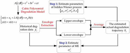
4. Subjective Parameter Estimation Based on Envelope Extraction

The parameters of a nonlinear Wiener process with a ME are commonly estimated by the MLE method. However, sometimes, the estimated parameters may not be able to reproduce the original data well. The reason is that the estimated parameters are based on the MLE of the selected mathematical model. However, there may exist a modeling error between the mathematical model and the actual degradation data. Therefore, it is unnecessarily optimal to use MLE directly for parameter estimation, especially when the modeling error is significant. It could also sometimes obtain a negative variance of the ME.

To address this issue, this section proposes a subjective parameter estimation method based on envelope extraction in two steps. That is, Step 1: estimate the parameters of the Wiener process; Step 2: estimate the parameter of the ME. The specific flowchart of this method is shown in Figure 2. Firstly, the upper and lower envelope curves of the lithium-ion batteries’ degradation data are calculated by envelope extraction. Secondly, the actual degradation trajectory is estimated by the average value of the upper and lower envelopes derived above. Then, the estimated actual degradation trajectory is used for parameter estimation of the hidden Wiener process. Secondly, the difference between the observed degradation data and the actual degradation trajectory is utilized to estimate the variance of the ME.

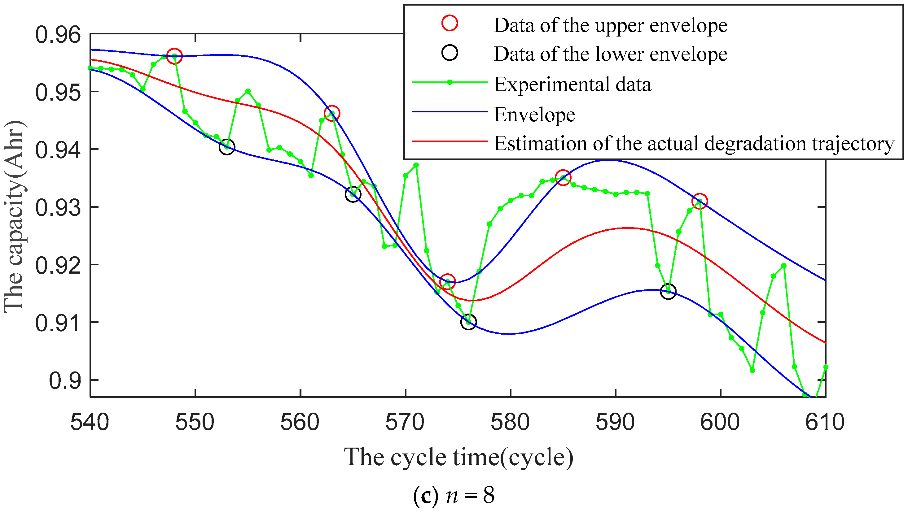
4.1. Estimation of Actual Degradation Trajectory of Lithium-Ion Batteries Based on Envelope Extraction

The purpose of envelope extraction is to estimate the actual degradation trajectory of lithium-ion batteries. Currently, signal envelope extraction is a relatively mature technology and has played an important role in many fields [53,54,55], which mainly include normalized Shannon entropy, the Hilbert transform, and the extreme value method.

Compared with traditional periodic signals, the degradation data of lithium-ion batteries shows non-periodic characteristics, a clear profile, and a monotonic decreasing trend. Therefore, this paper uses the extreme value method, with which it is relatively simple to calculate the envelope of lithium-ion batteries’ degradation data, and estimates the actual degradation trajectory of lithium-ion batteries by taking the average of the upper and lower envelopes. To offer greater clarity on the implementation of the proposed model, we give the corresponding steps in

Table 2. The specific steps of the envelope extraction algorithm.

Algorithm: Envelope Extraction
1. Calculate the Upper Envelope Curve. Collect the historical degradation data and search for local maximum $y_{i|\max }$. Select the regional maximum $p_{i|\max }$ from the specified interval $n$. Connect the selected data $p_{i|\max }$ with cubic spline interpolation.
2. Calculate the Lower Envelope Curve. Collect the historical degradation data and search for local minimum $y_{i|\min }$. Select the regional minimum $q_{i|\min }$ from the specified interval $n$. Connect the selected data $q_{i|\min }$ with cubic spline interpolation.
3. Estimate the Actual Degradation Trajectory. Calculate the average of the upper curves and lower envelope curves.

.

To capture the overall degradation trend of lithium batteries smoothly and accurately, the cubic spline interpolation method is used to connect the regional maximum $p_{i|\max }$ for the upper envelope curve and the regional minimum $q_{i|\min }$ for the lower envelope curve. This is because the cubic spline interpolation method has high computational accuracy, great convergence and accurate curve fitting. Additionally, its first and second derivatives are continuous, which produces a smooth connection at the interpolating points. For example, by using partial capacity degradation data of lithium-ion batteries and following the steps in Table 2, the estimated degradation trajectory under a different interval $n$ is shown in Figure 3. It can be observed that if the interval $n$ is set too small, it may not capture the overall degradation trend. If the interval $n$ is too large, many experimental data could be ignored, and the nonlinear trend of degradation could not be effectively captured. According to multiple experimental studies and subjective evaluation, we selected a specific interval n = 6, the experimental effect of which was optimal.

We could also observe that the average curve of the upper and lower envelope curves could reflect the actual degradation trajectory of lithium-ion battery with reasonable accuracy from the view of the Wiener degradation process. The reason is that in Wiener degradation with a ME, the Wiener process represents the hidden degradation trajectory that is smoother than the original degradation data and can capture hidden nonlinear degradation characteristics. Meanwhile, the ME represents the fluctuation of the observed degradation data. By dividing the traditional MLE method into two steps, the proposed subjective method can make the results of parameter estimation closer to the practical degradation data, which could further reduce the impact of modeling errors on parameter estimation.

4.2. Offline Parameters Estimation

The estimation of the actual degradation trajectory based on envelope extraction is mainly used for offline parameter estimation. Offline parameter estimation proposed in this paper is divided into two steps. The first step is to estimate the parameters of the hidden Wiener process based on the actual degradation trajectory estimated by envelope extraction. Generally, the cycle lengths of the historical degradation data of lithium-ion batteries are not equal. Therefore, the method of using the same measurement time interval for parameter estimation is not applicable, and an empirical parameter estimation method under different measurement times can be used for parameter estimation of the Wiener process [56]. Then, the parameters can be estimated in the following two steps:

Step 1: Estimate the parameters of the hidden Wiener process. Suppose that there are n lithium-ion batteries, and the actual capacity of the ith lithium-ion battery at different times $t_{i,1},t_{i,2},\cdots ,t_{i,m_i}$ can be represented as

$$x_{i,j}=X_i(t_{i,j})={\lambda }_i\Lambda (t_{i,j};\mathit{\theta })+{\sigma }_{B}B(t_{i,j})$$

(14)

where $1\le i\le n$ and $1\le j\le m_i$. Let $\Delta x_{i,j}=X_i(t_{i,j})-X_i(t_{i,j-1})$, and $\Delta x_{i,j}$ can be written as

$$\Delta x_{i,j}=X_i(t_{i,j})-X_i(t_{i,j-1})={\lambda }_i\Delta v_{i,j}+{\sigma }_{B}B(\Delta t_{i,j})$$

(15)

where $\Delta v_{i,j}=\Lambda (t_{i,j};\mathit{\theta })-\Lambda (t_{i,j-1};\mathit{\theta })$. Let $\Delta x_i={\left(\Delta x_{i,1},\Delta x_{i,2},\cdots ,\Delta x_{i,m_i}\right)}^{\prime }$, $\Delta {\nu }_i={\left(\Delta {\nu }_{i,1},\Delta {\nu }_{i,2},\cdots ,\Delta {\nu }_{i,m_i}\right)}^{\prime }$ and $\mathrm{X}={\left(\Delta x_1^{\prime },\Delta x_2^{\prime },\cdots ,\Delta x_n^{\prime }\right)}^{\prime }$. Then, ${\mathit{x}}_i$ follows the multivariate normal distribution, i.e., ${\mathit{x}}_i~N\left({\mu }_{\lambda }\Delta {\mathit{v}}_i,{\mathbf{\Sigma }}_i\right)$, where ${\mathbf{\Sigma }}_i={\sigma }_{\lambda }^2\Delta {\mathit{v}}_i\Delta {\mathit{v}}_i^{\prime }+{\sigma }_B^2{\Omega }_i$ and

$${\Omega }_i=\left[\begin{array}{cccc}\Delta t_{i,1}& 0& 0& 0\\ 0& \Delta t_{i,2}& 0& 0\\ 0& 0& \ddots & ⋮\\ 0& 0& \cdots & \Delta t_{i,m_i}\end{array}\right]$$

(16)

Hence, the log-likelihood function of the prior parameters $\mathbf{\Theta }=\left\{{\mu }_{\lambda },{\sigma }_{\lambda }^2,{\sigma }_B^2,\mathit{\theta }\right\}$ can be written as

$$\ln L(\mathbf{\Theta }|\mathbf{X})=-\frac{\ln 2\pi }{2}{\displaystyle \sum _{i=1}^n{m}_i}-\frac{1}{2}{\displaystyle \sum _{i=1}^n\ln \left|{\Sigma }_i\right|}-\frac{1}{2}{\displaystyle \sum _{i=1}^n{\left(\Delta {\mathit{x}}_i-{\mu }_{\lambda }\Delta {\mathit{v}}_i\right)}^{\prime }}{\mathbf{\Sigma }}_i^{-1}\left(\Delta {\mathit{x}}_i-{\mu }_{\lambda }\Delta {\mathit{v}}_i\right)$$

(17)

where $\left|{\mathbf{\Sigma }}_i\right|$ and ${\mathbf{\Sigma }}_i^{-1}$ can be calculated as follows.

$$\left|{\mathbf{\Sigma }}_i\right|=({\sigma }_B^2{)}^{m_i-1}\left({\sigma }_B^2+{\sigma }_{\lambda }^2\Delta {\mathit{v}}_i^{\prime }{\Omega }_i^{-1}\Delta {\mathit{v}}_i\right){\displaystyle \prod _{j=1}^{m_i}\Delta t_{i,j}}$$

(18)

$${\mathbf{\Sigma }}_i^{-1}=\frac{1}{{\sigma }_B^2}\left({\Omega }_i^{-1}-\frac{{\sigma }_{\lambda }^2}{{\sigma }_B^2+{\sigma }_{\lambda }^2\Delta {\mathit{v}}_i^{\prime }{\Omega }_i^{-1}\Delta {\mathit{v}}_i}{\Omega }_i^{-1}\Delta {\mathit{v}}_i\Delta {\mathit{v}}_i^{\prime }{\Omega }_i^{-1}\right)$$

(19)

By substituting Equations (18) and (19) into (17), we can obtain the profile likelihood function as follows.

$$\begin{array}{l}\ln L(\mathbf{\Theta }|X_{1:N})=-\frac{\ln 2\pi }{2}{\displaystyle \sum _{i=1}^n{m}_i}-\frac{\ln \left({\sigma }_B^2\right)}{2}{\displaystyle \sum _{i=1}^n\left(m_i-1\right)}-\frac{1}{2}{\displaystyle \sum _{i=1}^n\ln \left({\sigma }_B^2+{\sigma }_{\lambda }^2\Delta {\mathit{v}}_i^{\prime }{\Omega }_i^{-1}\Delta {\mathit{v}}_i\right)}-\frac{1}{2}{\displaystyle \sum _{i=1}^n{\displaystyle \sum _{j=1}^{m_i}\Delta t_{i,j}}}\\ \hspace{1em}\hspace{1em}\hspace{1em}\hspace{1em}-\frac{1}{2{\sigma }_B^2}{\displaystyle \sum _{i=1}^n\left(\Delta x_i^{\prime }{\Omega }_i^{-1}\Delta x_i-\frac{{\left(\Delta x_i^{\prime }{\Omega }_i^{-1}\Delta {\mathit{v}}_i\right)}^2}{\Delta {\mathit{v}}_i^{\prime }{\Omega }_i^{-1}\Delta {\mathit{v}}_i}\right)}-\frac{1}{2}{{\displaystyle \sum _{i=1}^n\frac{\Delta {\mathit{v}}_i^{\prime }{\Omega }_i^{-1}\Delta {\mathit{v}}_i}{{\sigma }_B^2+{\sigma }_{\lambda }^2\Delta {\mathit{v}}_i^{\prime }{\Omega }_i^{-1}\Delta {\mathit{v}}_i}\left({\mu }_{\lambda }-\frac{\Delta x_i^{\prime }{\Omega }_i^{-1}\Delta {\mathit{v}}_i}{\Delta {\mathit{v}}_i^{\prime }{\Omega }_i^{-1}\Delta {\mathit{v}}_i}\right)}}^2\end{array}$$

(20)

Due to the unequal lengths of the degradation data, it is difficult to obtain a closed-form expression for parameter estimation. In order to avoid falling into the local minimum during parameter searching, an empirical parameter estimation method can be used. Tang et al. [56] gave an empirical expression for parameter estimation based on the estimation results at the same measurement times. That is,

$${\widehat{\mu }}_{\lambda }\left(\mathit{\theta }\right)=\frac{1}{n}{\displaystyle \sum _{i=1}^n\frac{\Delta x_i^{\prime }{\Omega }_i^{-1}\Delta {\mathit{v}}_i}{\Delta {\mathit{v}}_i^{\prime }{\Omega }_i^{-1}\Delta {\mathit{v}}_i}}$$

(21)

$${\widehat{\sigma }}_{\lambda }^2\left(\mathit{\theta }\right)=\frac{1}{n}{\displaystyle \sum _{i=1}^n{\left({\widehat{\mu }}_{\lambda }-{\widehat{\lambda }}_i\right)}^2}-\frac{1}{n}{\displaystyle \sum _{i=1}^n\frac{{\left(\Delta {\mathit{x}}_i-{\widehat{\lambda }}_i\Delta {\mathit{v}}_i\right)}^{\prime }{\Omega }_i^{-1}\left(\Delta {\mathit{x}}_i-{\widehat{\lambda }}_i\Delta {\mathit{v}}_i\right)}{\left(m_i-1\right)\Delta {\mathit{v}}_i^{\prime }{\Omega }_i^{-1}\Delta {\mathit{v}}_i}}$$

(22)

$${\widehat{\sigma }}_B^2\left(\mathit{\theta }\right)=\frac{1}{n}{\displaystyle \sum _{i=1}^n\frac{{\left(\Delta {\mathit{x}}_i-{\widehat{\lambda }}_i\Delta {\mathit{v}}_i\right)}^{\prime }{\Omega }_i^{-1}\left(\Delta {\mathit{x}}_i-{\widehat{\lambda }}_i\Delta {\mathit{v}}_i\right)}{\left(m_i-1\right)}}$$

(23)

where ${\widehat{\lambda }}_i=\frac{\Delta {\mathit{x}}_i^{\prime }{\Omega }_i^{-1}\Delta v_i}{\Delta {v^{\prime }}_i{\Omega }_i{}^{-1}\Delta {\mathit{v}}_i}$, $\Delta {\nu }_i$ is the ith term of $\Delta \nu$, and ${\Omega }_i$ is the ith term of $\Omega$.

By substituting Equations (21)–(23) into Equation (20) and maximizing it, we can obtain the estimated value of $\mathit{\theta }$, i.e., $\widehat{\mathit{\theta }}=\left\{\widehat{b},\widehat{c}\right\}$. Then, by substituting the estimated value of $\widehat{\mathit{\theta }}=\left\{\widehat{b},\widehat{c}\right\}$ into Equations (21)–(23), we can obtain the estimation of parameters ${\widehat{\mu }}_{\lambda }\left(\widehat{\mathit{\theta }}\right)$, ${\widehat{\sigma }}_{\lambda }^2\left(\widehat{\mathit{\theta }}\right)$, and ${\widehat{\sigma }}_B^2\left(\widehat{\mathit{\theta }}\right)$. It is worth noting that ${\widehat{\mu }}_{\lambda }\left(\widehat{\mathit{\theta }}\right)$ and ${\widehat{\sigma }}_B^2\left(\mathit{\theta }\right)$ are unbiased estimations, while ${\widehat{\sigma }}_{\lambda }^2\left(\mathit{\theta }\right)$ is a biased estimation. The unbiased estimation of ${\widehat{\sigma }}_{\lambda }^2\left(\mathit{\theta }\right)$ can be calculated based on the following equation.

$${\widehat{\sigma }}_{\lambda }^2\left(\mathit{\theta }\right)=\frac{1}{n-1}{\displaystyle \sum _{i=1}^n{\left({\widehat{\mu }}_{\lambda }-{\widehat{\lambda }}_i\right)}^2}-\frac{1}{n}{\displaystyle \sum _{i=1}^n\frac{{\left(\Delta {\mathit{x}}_i-{\widehat{\lambda }}_i\Delta {\mathit{v}}_i\right)}^{\prime }{\Omega }_i^{-1}\left(\Delta {\mathit{x}}_i-{\widehat{\lambda }}_i\Delta {\mathit{v}}_i\right)}{\left(m_i-1\right)\Delta {\mathit{v}}_i^{\prime }{\Omega }_i^{-1}\Delta {\mathit{v}}_i}}$$

(24)

Step 2: Estimate the parameter of the ME. The variance of the ME is estimated based on the actual degradation trajectory of lithium-ion batteries estimated by the average value of the upper and lower envelope curves. Since the ME is independent with the drift coefficient and Brownian motion, its variance can be estimated as

$${\sigma }_{\epsilon }^2=\frac{1}{n}{\displaystyle \sum _{i=1}^n{\displaystyle \sum _{j=1}^{m_i}\frac{{(y_{i,j}-x_{i,j})}^2}{m_i-1}}}$$

(25)

where $x_{i,j}$ is the estimated actual capacity of the ith lithium-ion battery in the jth cycle, and $y_{i,j}$ is the original observed capacity obtained from the ith lithium-ion battery in the jth cycle.

5. Experimental Studies

This section validates the effectiveness and practicality of the subjective parameter estimation method and the cubic polynomial function model based on the practical degradation data of lithium-ion batteries. First, the proposed subjective parameter estimation method was validated through simulation experiments. Then, the effectiveness of envelope extraction and the cubic polynomial function model were experimentally verified with practical degradation data of lithium-ion batteries.

5.1. Offline Parameter Estimation

In this section, the proposed method is validated using the capacity degradation data from the Center for Advanced Life Cycle Engineering (CALCE) of the University of Maryland [29,48,49]. All battery tests were conducted under ambient conditions at 25 °C. In the process of charging, the batteries underwent a constant current charge of 0.5 C until the voltage reached 4.2 V, followed by a constant voltage charge at 4.2 V until the current decreased to 0.05 A. In the process of discharging, these batteries were discharged to 2.7 V with a current of 1 C. The experimental data were generated by a group of four lithium-ion batteries with a nominal capacity of 1.1 Ahr, as shown in Figure 4. The CS237 lithium-ion battery was selected as the unit to be evaluated, and the remaining experimental data were used for prior parameter estimation. The subjective parameter estimation method based on envelope extraction was used to estimate the actual degradation trajectory, as shown in Figure 5. It can be observed that the actual degradation trajectory obtained in this paper was similar to that in [48]. These two smoothed graphs could both capture the nonlinear degradation characteristic of the capacity. However, this study’s degradation data of the battery in Figure 5 was smoother and thus better than that in [48].

In order to compare with traditional MLE methods with a ME [44], the Akaike information criterion (AIC) was introduced as a standard for evaluating the fitting effectiveness of different parameter estimation methods. That is,

$$\mathrm{AIC}=2(k-\ln L(\Theta ))$$

(26)

where k is the number of model parameters.

For simplicity, the method proposed in this paper is denoted as M₀, and the traditional MLE method with a ME is denoted as M₁. The parameter estimation results obtained by these two methods are shown in

Table 3. The estimated parameters of M₀ and M₁.

Method	M0	M1
${\mu }_1$	2.42 × 10−9	3.21 × 10−9
${\sigma }_{\lambda }^2$	2.96 × 10−19	6.07 × 10−19
${\sigma }_B^2$	1.95 × 10−6	5.14 × 10−5
${\sigma }_{\epsilon }^2$	5.02 × 10−5	−5.16 × 10−6
b	−9.57 × 102	−1.01 × 103
c	3.93 × 105	3.91 × 105
LnL	1.45 × 104	6.18e × 103
AIC	−2.90 × 104	−1.24 × 104

. It can be observed that M₀ had a smaller AIC than M₁ did, indicating a better fit. This was because the estimated degradation trajectory obtained by envelope extraction was relatively smooth compared to the measurement data, which led to better fitting performance during the fitting process.

To further compare the effectiveness of parameter estimation by these two methods, a simulation experiment with simulated degradation data was implemented. The difference between the original degradation data and the simulated degradation data reflected the model fitting ability of the different methods. The degradation data was simulated based on the nonlinear Wiener process with a ME under the estimated parameters obtained in Table 3. Specifically, the nonlinear function was first calculated by the cubic polynomial function. Then, Brownian movement and the ME were simulated, respectively. By adding up these three parts, the degradation data could be simulated. By setting the detection cycle to 800 and the detection time interval to 1, 10 sets of degradation data were simulated based on the estimation results by M₀, as shown in Figure 6. Similarly, we obtain the simulated data by M₁, as shown in Figure 7.

It can be observed that the degradation data estimated by M₀ had a smaller diffusion range and were closer to the measurement data. The simulated data of M₁ had a relatively larger diffusion range. It could be explained by the fact that ${\sigma }_B^2$ estimated by M₁ was larger than that estimated by M₀. That is, the parameter ${\sigma }_B^2$ was overestimated by M₁. It could further be overwhelmed by the nonlinear characteristics of the degradation data and make it difficult to capture the potential nonlinear characteristics of the degradation process. It can also be observed that the degradation trajectory estimated by the subjective parameter estimation method was smoother than the original measured data. It indicates that this method was beneficial for capturing potential nonlinear characteristics of the degradation trajectory and reducing the impact of modeling error on the estimation results of traditional MLE. To make a quantitative analysis, MSE_M were calculated based on the data simulated by M₀ and M₁ using Equation (4). The results were 3.90 × 10⁻⁴ for M₀ and 3.08 × 10⁻³ for M₁, respectively. It could be obtained that the simulation experiment data of M₀ had a smaller MSE_M, indicating that the results simulated with M₀ could more accurately reflect the degradation state.

5.2. RUL Prediction

This subsection mainly validates the effectiveness of the proposed method for RUL prediction. Generally, lithium-ion batteries are considered to have failed when battery capacities are lower than 70–80% of the rated capacity. In this paper, it was assumed that the failure threshold for lithium-ion batteries was 75% (0.825 Ahr) of the rated capacity. Take battery CS237 as an example. Its capacity corresponding to 75% of the rated capacity was at the 643th cycle, so its actual lifetime was 643 cycles.

The PDFs of RUL calculated by M₀ and M₁ at different cycles are shown in Figure 8. The PDF of RUL at the 570th cycle is shown in Figure 9. It can be observed that although both methods could cover the actual RUL, the PDF of RUL estimated by M₀ was narrower and more concentrated around the actual RUL than that estimated by M₁. This was because the estimated actual degradation trajectory based on envelope extraction was smoother, resulting in a smaller estimation of ${\sigma }_B^2$. It could obtain a narrow confidence interval with more accuracy. This indicates that the estimation of the actual degradation trajectory by M₀ fit the nonlinear characteristics of the degradation process better. Additionally, the estimated uncertainty of the actual degradation trajectory by M₀ was smaller. Therefore, it could be concluded that M₀ could obtain a closer RUL and reduce the uncertainty of RUL prediction, which demonstrated that the accuracy of RUL prediction by M₀ was improved.

In order to compare the prediction performance of these two methods from a quantitative perspective, the mean squared error (MSE) of RUL prediction was used for comparison. That is,

$$MS{E}_k={\displaystyle {\int }_0^{\infty }{\left(l_k+t_k-T\right)}^2{f}_{L_k|Y_{0:k}}\left(l_k|Y_{0:k}\right)d{l}_k}$$

(27)

where $T$ represents the actual lifetime of the tested equipment, $l_k$ represents the RUL at time $t_k$, and $f_{L_k\left|Y_{0:k}\right.}(l_k\left|Y_{0:k}\right.)$ represents the estimated PDF of RUL at time $t_k$. The MSEs calculated by these two methods are shown in Figure 10, and it can be observed that the MSEs of M₀ were much smaller than those of M₁. This further illustrates that M₀ could effectively improve the accuracy of RUL prediction of lithium-ion batteries.

The above experimental studies have demonstrated the effectiveness of the subjective parameter estimation method based on envelope extraction. Next, RUL prediction performance of a cubic polynomial function and other nonlinear functions were compared. The cubic polynomial function degradation model $\Lambda \left(t;\mathit{\theta }\right)=t^3+b{t}^2+ct$ was denoted as M₀. The typical four nonlinear models for comparison were $\Lambda \left(t;\mathit{\theta }\right)=\exp (bt)+c\exp (dt)$, $\Lambda \left(t;\mathit{\theta }\right)=\exp (bt)-1$, $\Lambda \left(t;\mathit{\theta }\right)=t^b$, and $\Lambda \left(t;\mathit{\theta }\right)=\exp (bt)+c{t}^2$, which were denoted as M₂, M₃, M₄, and M₅, respectively. The parameter estimation results based on these nonlinear models are shown in

Table 4. Parameter estimation results of different nonlinear models.

Method	M0	M2	M3	M4	M5
${\mu }_1$	2.42 × 10−9	4.04 × 10−2	4.05 × 10−2	2.87 × 10−11	−3.82 × 10−6
${\sigma }_{\lambda }^2$	2.96 × 10−19	7.25 × 10−5	7.26 × 10−5	3.79 × 10−23	3.17 × 10−7
${\sigma }_B^2$	1.96 × 10−6	2.04 × 10−6	2.04 × 10−6	2.05 × 10−6	2.16 × 10−6
b	−9.87 × 102	3.26 × 10−3	3.26 × 10−6	3.54 × 10−6	−1.72 × 106
c	3.93 × 105	1.34 × 10−4	-	-	−2.57 × 10−4
d	-	1.23 × 10−6	-	-	-
Ln L	1.45 × 104	1.44 × 104	1.38 × 104	1.44 × 104	1.44 × 104
AIC	−2.90 × 104	−2.89 × 104	−2.76 × 104	−2.89 × 104	−2.87 × 104

. We could observe that, compared with those of other nonlinear models, M₀ had the smallest AIC, indicating that it had the best fit.

In order to intuitively compare the RUL prediction of the different models, the PDFs of RUL M₀ at different cycles were calculated and shown in Figure 11. It could be observed that all five models could completely cover the actual RUL. However, compared with those of the other four typical nonlinear models, M₀ had the highest PDF of RUL and was closest to the actual RUL under different cycles.

For illustrative purposes, we calculated the PDF of RUL at the 555th cycle, the actual RUL of which was 88 cycles, as shown in Figure 12. It could be observed that compared with that of the other four models, M₀ had a narrower and more concentrated PDF of RUL near the actual RUL. Combining the fitting performance of M₀ as shown in Figure 1, it could be observed that M₃, M₄, and M₅ had slow degradation rates and could not fit the rapid degradation characteristics of lithium-ion batteries in the last stage, which resulted in overestimation of remaining life by M₃, M₄, and M₅ and caused the PDF to deviate from the actual RUL and shift to the right of the abscissa axis. Although M₂ could fit the last stage of the degradation rate, its degradation model only considered the rapid decrease of the last stage of the degradation rate without the overall degradation process. As a result, although the PDF of M₂ was concentrated and near the actual state of degradation, its uncertainty was higher than that of M₀. It could result in a relatively lower height of PDF and larger uncertainty of RUL prediction.

In order to further quantify the superiority of the proposed method, the MSEs of these five models for RUL prediction were calculated, as shown in Figure 13. It could be observed that the MSEs of M₀ proposed in this paper were smaller than those of models M₂, M₃, M₄, and M₅. It indicates that the nonlinear degradation model established by the cubic polynomial function was more in line with the degradation characteristics of lithium-ion batteries and could improve the accuracy of RUL prediction.

Additionally, another cross validation was done for RUL prediction. As when battery CS237 was selected as the unit to be evaluated and the other three batteries were used for prior parameter estimation, we repeated this experimental study four times by selecting a different battery for testing. The total MSE by adding up the MSEs of each cycle is displayed in

Table 5. The total MSEs of RUL for different methods.

Selected Battery	M0	M1	M2	M3	M4	M5
CS 235	1.62 × 106	9.82 × 106	3.07 × 106	8.12 × 106	3.43 × 107	4.92 × 107
CS 236	6.32 × 106	9.94 × 107	2.08 × 107	2.06 × 107	5.82 × 107	3.24 × 107
CS 237	2.18 × 106	1.19 × 107	4.43 × 106	7.16 × 106	2.22 × 107	4.24 × 107
CS 238	6.51 × 106	1.98 × 107	6.70 × 106	1.21 × 107	2.46 × 107	4.14 × 107

. It could be observed that the results were similar to those of battery CS237. This further showed the robustness of the proposed method.

6. Conclusions

Accurately establishing a degradation model and conducting effective parameter estimation are prerequisites for ensuring the accuracy of RUL prediction of lithium-ion batteries. Since the existing degradation models based on the Wiener process are relatively simple and the effectiveness of parameters estimation is insufficient, this paper proposes a degradation model based on a cubic polynomial function and a subjective parameter estimation method based on envelope extraction. Firstly, based on the typical characteristics of the degradation process of lithium-ion batteries and existing degradation models, a cubic polynomial function model was selected as the nonlinear function for the Wiener process. Secondly, a subjective parameter estimation method based on envelope extraction was proposed to obtain smooth degradation trajectories of lithium-ion batteries. Finally, the effectiveness of the proposed method in improving the accuracy of RUL prediction was validated through simulation experiments and practical degradation data of lithium-ion batteries.

The summary of the main contributions of this paper is as follows:

(1)

A method based on envelope extraction was proposed to estimate the degradation trajectory, and algorithms for obtaining the upper/lower envelope curves and an expression for the estimation of the ME were proposed. The effectiveness and practicality of this method were validated through comparisons with traditional MLE methods considering the ME in terms of MSE_M.

(2)

The degradation trajectory was fitted using a cubic polynomial function model based on nonlinear Wiener processes. Through comparison and analysis with several typical nonlinear models, it was demonstrated that the cubic polynomial function model fit the typical degradation characteristics of lithium-ion batteries better and could improve the accuracy of RUL prediction for lithium-ion batteries in terms of MSE of RUL prediction.

In the future, we will focus on the physical models and ambient conditions such as temperature, charge current, and discharge current for predicting the RUL, as this is a valuable direction in improving the accuracy of prognostics of lithium-ion batteries. Additionally, the generality of a cubic polynomial degradation model is worth further researching.

References

1. Tian, H.; Qin, P.; Li, K.; Zhao, Z. A review of the state of health for lithium-ion batteries: Research status and suggestions. J. Clean. Prod. 2020, 261, 120813. [Google Scholar] [CrossRef]
2. Wang, S.; Jin, S.; Bai, D.; Fan, Y.; Shi, H.; Fernandez, C. A critical review of improved deep learning methods for the remaining useful life prediction of lithium-ion batteries. Energy Rep. 2021, 7, 5562–5574. [Google Scholar] [CrossRef]
3. Dai, Q.; Kelly, J.C.; Gaines, L.; Wang, M. Life cycle analysis of lithium-ion batteries for automotive applications. Batteries 2019, 5, 48. [Google Scholar] [CrossRef]
4. Kurzweil, P.; Shamonin, M. State-of-charge monitoring by impedance spectroscopy during long-term self-discharge of supercapacitors and Lithium-Ion batteries. Batteries 2018, 4, 35. [Google Scholar] [CrossRef]
5. Liu, K.; Shang, Y.; Ouyang, Q.; Widanage, W.D. A data-driven approach with uncertainty quantification for predicting future capacities and remaining useful life of lithium-ion battery. IEEE Trans. Ind. Electron. 2021, 68, 3170–3180. [Google Scholar] [CrossRef]
6. Tomaszewska, A.; Chu, Z.; Feng, X.; O’kane, S.; Liu, X.; Chen, J.; Ji, C.; Endler, E.; Li, R.; Liu, L. Lithium-ion battery fast charging: A review. ETransportation 2019, 1, 100011. [Google Scholar] [CrossRef]
7. Pecht, M. Prognostics and health management of electronics. In Encyclopedia of Structural Health Monitoring; Wiley & Sons: New York, NY, USA, 2009. [Google Scholar] [CrossRef]
8. Meng, H.; Li, Y.-F. A review on prognostics and health management (PHM) methods of lithium-ion batteries. Renew. Sustain. Energy Rev. 2019, 116, 109405. [Google Scholar] [CrossRef]
9. Li, Y.; Liu, K.; Foley, A.M.; Zülke, A.; Berecibar, M.; Nanini-Maury, E.; Van Mierlo, J.; Hoster, H.E. Data-driven health estimation and lifetime prediction of lithium-ion batteries: A review. Renew. Sustain. Energy Rev. 2019, 113, 109254. [Google Scholar] [CrossRef]
10. Hu, X.; Xu, L.; Lin, X.; Pecht, M. Battery Lifetime Prognostics. Joule 2020, 4, 310–346. [Google Scholar] [CrossRef]
11. Ochella, S.; Shafiee, M.; Dinmohammadi, F. Artificial intelligence in prognostics and health management of engineering systems. Eng. Appl. Artif. Intell. 2022, 108, 104552. [Google Scholar] [CrossRef]
12. Xia, Q.; Wang, Z.; Ren, Y.; Tao, L.; Lu, C.; Tian, J.; Hu, D.; Wang, Y.; Su, Y.; Chong, J.; et al. A modified reliability model for lithium-ion battery packs based on the stochastic capacity degradation and dynamic response impedance. J. Power Sources 2019, 423, 40–51. [Google Scholar] [CrossRef]
13. Sgroi, M.F. Lithium-ion batteries aging mechanisms. Batteries 2022, 8, 205. [Google Scholar] [CrossRef]
14. Tran, M.-K.; DaCosta, A.; Mevawalla, A.; Panchal, S.; Fowler, M. Comparative study of equivalent circuit models performance in four common lithium-ion batteries: LFP, NMC, LMO, NCA. Batteries 2021, 7, 51. [Google Scholar] [CrossRef]
15. Yu, W.; Guo, Y.; Shang, Z.; Zhang, Y.; Xu, S. A review on comprehensive recycling of spent power lithium-ion battery in China. Etransportation 2022, 11, 100155. [Google Scholar] [CrossRef]
16. Su, L.; Wu, M.; Li, Z.; Zhang, J. Cycle life prediction of lithium-ion batteries based on data-driven methods. ETransportation 2021, 10, 100137. [Google Scholar] [CrossRef]
17. Lei, Y.; Li, N.; Guo, L.; Li, N.; Yan, T.; Lin, J. Machinery health prognostics: A systematic review from data acquisition to RUL prediction. Mech. Syst. Signal Process. 2018, 104, 799–834. [Google Scholar] [CrossRef]
18. Meng, J.; Azib, T.; Yue, M. Early-Stage end-of-Life prediction of lithium-Ion battery using empirical mode decomposition and particle filter. Proc. Inst. Mech. Eng. Part A J. Power Energy 2023, 237, 1090–1099. [Google Scholar] [CrossRef]
19. Zhang, Y.; Xiong, R.; He, H.; Pecht, M.G. Long Short-Term Memory Recurrent Neural Network for Remaining Useful Life Prediction of Lithium-Ion Batteries. IEEE Trans. Veh. Technol. 2018, 67, 5695–5705. [Google Scholar] [CrossRef]
20. Liu, D.; Zhou, J.; Pan, D.; Peng, Y.; Peng, X. Lithium-ion battery remaining useful life estimation with an optimized Relevance Vector Machine algorithm with incremental learning. Measurement 2015, 63, 143–151. [Google Scholar] [CrossRef]
21. Zhang, Y.; Xiong, R.; He, H.; Pecht, M. Validation and verification of a hybrid method for remaining useful life prediction of lithium-ion batteries. J. Clean. Prod. 2019, 212, 240–249. [Google Scholar] [CrossRef]
22. Liu, K.; Li, Y.; Hu, X.; Lucu, M.; Widanage, W.D. Gaussian process regression with automatic relevance determination kernel for calendar aging prediction of lithium-ion batteries. IEEE Trans. Ind. Inform. 2020, 16, 3767–3777. [Google Scholar] [CrossRef]
23. Li, X.; Zhang, L.; Wang, Z.; Dong, P. Remaining useful life prediction for lithium-ion batteries based on a hybrid model combining the long short-term memory and Elman neural networks. J. Energy Storage 2019, 21, 510–518. [Google Scholar] [CrossRef]
24. Lipu, M.S.H.; Hannan, M.A.; Hussain, A.; Hoque, M.M.; Ker, P.J.; Saad, M.H.M.; Ayob, A. A review of state of health and remaining useful life estimation methods for lithium-ion battery in electric vehicles: Challenges and recommendations. J. Clean. Prod. 2018, 205, 115–133. [Google Scholar] [CrossRef]
25. Bae, S.J.; Kvam, P.H. A nonlinear random-coefficients model for degradation testing. Technometrics 2004, 46, 460–469. [Google Scholar] [CrossRef]
26. Lu, C.J.; Meeker, W.O. Using degradation measures to estimate a time-to-failure distribution. Technometrics 1993, 35, 161–174. [Google Scholar] [CrossRef]
27. Gebraeel, N.Z.; Lawley, M.A.; Li, R.; Ryan, J.K. Residual-life distributions from component degradation signals: A Bayesian approach. IiE Trans. 2005, 37, 543–557. [Google Scholar] [CrossRef]
28. Su, C.; Lu, J.-C.; Chen, D.; Hughes-Oliver, J.M. A random coefficient degradation model with ramdom sample size. Lifetime Data Anal. 1999, 5, 173–183. [Google Scholar] [CrossRef]
29. He, W.; Williard, N.; Osterman, M.; Pecht, M. Prognostics of lithium-ion batteries based on Dempster–Shafer theory and the Bayesian Monte Carlo method. J. Power Sources 2011, 196, 10314–10321. [Google Scholar] [CrossRef]
30. Chen, L.; An, J.; Wang, H.; Zhang, M.; Pan, H. Remaining useful life prediction for lithium-ion battery by combining an improved particle filter with sliding-window gray model. Energy Rep. 2020, 6, 2086–2093. [Google Scholar] [CrossRef]
31. Zhang, Y.; Chen, L.; Li, Y.; Zheng, X.; Chen, J.; Jin, J. A hybrid approach for remaining useful life prediction of lithium-ion battery with Adaptive Levy Flight optimized Particle Filter and Long Short-Term Memory network. J. Energy Storage 2021, 44, 103245. [Google Scholar] [CrossRef]
32. Ma, G.; Wang, Z.; Liu, W.; Fang, J.; Zhang, Y.; Ding, H.; Yuan, Y. A two-stage integrated method for early prediction of remaining useful life of lithium-ion batteries. Knowl. Based Syst. 2023, 259, 110012. [Google Scholar] [CrossRef]
33. Hu, C.; Ye, H.; Jain, G.; Schmidt, C. Remaining useful life assessment of lithium-ion batteries in implantable medical devices. J. Power Sources 2018, 375, 118–130. [Google Scholar] [CrossRef]
34. Su, X.; Wang, S.; Pecht, M.; Zhao, L.; Ye, Z. Interacting multiple model particle filter for prognostics of lithium-ion batteries. Microelectron. Reliab. 2017, 70, 59–69. [Google Scholar] [CrossRef]
35. Xing, Y.; Ma, E.W.M.; Tsui, K.-L.; Pecht, M. An ensemble model for predicting the remaining useful performance of lithium-ion batteries. Microelectron. Reliab. 2013, 53, 811–820. [Google Scholar] [CrossRef]
36. Wang, R.; Zhu, M.; Zhang, X.; Pham, H. Lithium-ion battery remaining useful life prediction using a two-phase degradation model with a dynamic change point. J. Energy Storage 2023, 59, 106457. [Google Scholar] [CrossRef]
37. Micea, M.V.; Ungurean, L.; Cârstoiu, G.N.; Groza, V. Online state-of-health assessment for battery management systems. IEEE Trans. Instrum. Meas. 2011, 60, 1997–2006. [Google Scholar] [CrossRef]
38. Zhang, M.; Kang, G.; Wu, L.; Guan, Y. A method for capacity prediction of lithium-ion batteries under small sample conditions. Energy 2022, 238, 122094. [Google Scholar] [CrossRef]
39. Sun, Y.; Hao, X.; Pecht, M.; Zhou, Y. Remaining useful life prediction for lithium-ion batteries based on an integrated health indicator. Microelectron. Reliab. 2018, 88–90, 1189–1194. [Google Scholar] [CrossRef]
40. Chen, D.; Meng, J.; Huang, H.; Wu, J.; Liu, P.; Lu, J.; Liu, T. An empirical-data hybrid driven approach for remaining Useful Life prediction of lithium-ion batteries considering capacity diving. Energy 2022, 245, 123222. [Google Scholar] [CrossRef]
41. Ansari, S.; Ayob, A.; Hossain Lipu, M.S.; Hussain, A.; Saad, M.H.M. Remaining useful life prediction for lithium-ion battery storage system: A comprehensive review of methods, key factors, issues and future outlook. Energy Rep. 2022, 8, 12153–12185. [Google Scholar] [CrossRef]
42. Xu, X.; Tang, S.; Yu, C.; Xie, J.; Han, X.; Ouyang, M. Remaining useful life prediction of lithium-ion batteries based on Wiener process under time-varying temperature condition. Reliab. Eng. Syst. Saf. 2021, 214, 107675. [Google Scholar] [CrossRef]
43. Feng, L.; Wang, H.; Si, X.; Zou, H. A state-space-based prognostic model for hidden and age-dependent nonlinear degradation process. IEEE Trans. Autom. Sci. Eng. 2013, 10, 1072–1086. [Google Scholar] [CrossRef]
44. Han, Y.; Ma, C.; Tang, S.; Wang, F.; Sun, X.; Si, X. Residual life estimation of lithium-ion batteries based on nonlinear Wiener process with measurement error. Proc. Inst. Mech. Eng. Part O J. Risk Reliab. 2022, 237, 133–151. [Google Scholar] [CrossRef]
45. Jin, G.; Matthews, D.E.; Zhou, Z. A Bayesian framework for on-line degradation assessment and residual life prediction of secondary batteries inspacecraft. Reliab. Eng. Syst. Saf. 2013, 113, 7–20. [Google Scholar] [CrossRef]
46. Tang, S.; Guo, X.; Zhou, Z. Mis-specification analysis of linear Wiener process–based degradation models for the remaining useful life estimation. Proc. Inst. Mech. Eng. Part O J. Risk Reliab. 2014, 228, 478–487. [Google Scholar] [CrossRef]
47. Tang, S.; Yu, C.; Wang, X.; Guo, X.; Si, X. Remaining useful life prediction of lithium-ion batteries based on the Wiener process with measurement error. Energies 2014, 7, 520–547. [Google Scholar] [CrossRef]
48. Chen, X.; Liu, Z. A long short-term memory neural network based Wiener process model for remaining useful life prediction. Reliab. Eng. Syst. Saf. 2022, 226, 108651. [Google Scholar] [CrossRef]
49. Battery Research Data. Available online: https://calce.umd.edu/data (accessed on 5 April 2023).
50. Zheng, J.F.; Si, X.S.; Hu, C.H.; Zhang, Z.X.; Jiang, W. A nonlinear prognostic model for degrading systems with three-source variability. IEEE Trans. Reliab. 2016, 65, 736–750. [Google Scholar] [CrossRef]
51. Yu, W.; Tu, W.; Kim, I.Y.; Mechefske, C. A nonlinear-drift-driven Wiener process model for remaining useful life estimation considering three sources of variability. Reliab. Eng. Syst. Saf. 2021, 212, 107631. [Google Scholar] [CrossRef]
52. Tang, S. Research on Availability Assessment and Remaining Useful Life Estimation for Storage Systems. Ph.D. Dissertation, High-Tech Institute, Xi’an, China, 2015. [Google Scholar]
53. Borghesani, P.; Ricci, R.; Chatterton, S.; Pennacchi, P. A new procedure for using envelope analysis for rolling element bearing diagnostics in variable operating conditions. Mech. Syst. Signal Process. 2013, 38, 23–35. [Google Scholar] [CrossRef]
54. Yang, Y.; Yu, D.; Cheng, J. A fault diagnosis approach for roller bearing based on IMF envelope spectrum and SVM. Measurement 2007, 40, 943–950. [Google Scholar] [CrossRef]
55. Nguyen, P.; Kang, M.; Kim, J.-M.; Ahn, B.-H.; Ha, J.-M.; Choi, B.-K. Robust condition monitoring of rolling element bearings using de-noising and envelope analysis with signal decomposition techniques. Expert Syst. Appl. 2015, 42, 9024–9032. [Google Scholar] [CrossRef]
56. Tang, S.; Wang, F.; Sun, X.; Xu, X.; Yu, C.; Si, X. Unbiased parameters estimation and mis-specification analysis of Wiener process-based degradation model with random effects. Appl. Math. Model. 2022, 109, 134–160. [Google Scholar] [CrossRef]
Figure 1. Fitting degradation data of Battery CS235 with different degradation models.
Batteries 09 00441 g001
Figure 2. The flowchart of the method based on envelope extraction.
Batteries 09 00441 g002
Figure 3. Estimation of the actual degradation trajectory of lithium-ion batteries.
Batteries 09 00441 g003aBatteries 09 00441 g003b
Figure 4. Capacity degradation data of lithium-ion batteries [49].
Batteries 09 00441 g004
Figure 5. The estimated actual degradation data of lithium-ion batteries based on envelope extraction.
Batteries 09 00441 g005
Figure 6. Degradation trajectories simulated by M0.
Batteries 09 00441 g006
Figure 7. Degradation trajectories simulated by M1.
Batteries 09 00441 g007
Figure 8. PDFs of RUL at different cycles by M0 and M1.
Batteries 09 00441 g008
Figure 9. Distribution of RUL at the 570th cycle.
Batteries 09 00441 g009
Figure 10. The MSEs of RUL for methods M0 and M1.
Batteries 09 00441 g010
Figure 11. PDFs of RUL at different cycles by M0, M2, M3, M4 and M5.
Batteries 09 00441 g011
Figure 12. The distribution of RUL for the 555th cycle.
Batteries 09 00441 g012
Figure 13. The MSEs of RUL for methods M0, M2, M3, M4, and M5.
Batteries 09 00441 g013