Article

Introducing the Loewner Method as a Data-Driven and Regularization-Free Approach for the Distribution of Relaxation Times Analysis of Lithium-Ion Batteries

1
Chair for Electrical Energy Systems, University of Bayreuth, Universitätsstraße 30, 95447 Bayreuth, Germany
2
Bavarian Center for Battery Technology, University of Bayreuth, Universitätsstraße 30, 95447 Bayreuth, Germany
3
Max Planck Institute for Dynamics and Complex Technical Systems, Sandtorstraße 1, 39106 Magdeburg, Germany
4
Electrical and Computer Engineering Department, Rice University, 6100 Mainstreet, Houston, TX 77005, USA
*
Author to whom correspondence should be addressed.
Batteries 2023, 9(2), 132; https://doi.org/10.3390/batteries9020132
Submission received: 13 January 2023 / Revised: 7 February 2023 / Accepted: 9 February 2023 / Published: 13 February 2023
(This article belongs to the Special Issue Feature Papers to Celebrate the First Impact Factor of Batteries)

Abstract

:
For the identification of processes in lithium-ion batteries (LIB) by electrochemical impedance spectroscopy, frequency data is often transferred into the time domain using the method of distribution of relaxation times (DRT). As this requires regularization due to the ill-conditioned optimization problem, the investigation of data-driven methods becomes of interest. One promising approach is the Loewner method (LM), which has already had a number of applications in different fields of science but has not been applied to batteries yet. In this work, it is first deployed on synthetic data with predefined time constants and gains. The results are analyzed concerning the choice of model order, the type of processes , i.e., distributed and discrete, and the signal-to-noise ratio. Afterwards, the LM is used to identify and analyze the processes of a cylindrical LIB. To verify the results of this assessment a comparison is made with the generalized DRT at two different states of health of the LIB. It is shown that both methods lead to the same qualitative results. For the assignment of processes as well as for the interpretation of minor gains, the LM shows advantageous behavior, whereas the generalized DRT shows better results for the determination of lumped elements and resistive–inductive processes.

1. Introduction

Electrochemical impedance spectroscopy (EIS) is a state-of-the-art method for the non-destructive characterization and analysis of electrochemical systems. Typical applications for energy systems are fuel cells [1,2], lithium-ion batteries [3,4,5] (LIB), and double-layer capacitors [6,7]. This technique was utilized for the analysis of individual frequency-dependent processes [8] and the behavior of characteristic features of the whole spectrum [9,10,11]. Applications include the estimation of the state of charge (SOC) [12,13], the state of health [12,14], the internal temperature [8,12], or the detection of lithium plating [15,16,17].
For post-processing and interpretation of impedance data, the distribution of relaxation times (DRT) and the analysis of physical impedance models are the most prominent methods. A comprehensive overview of impedance modeling is given by Gaddam et al. in [18]. Different equivalent circuit models (ECM) are discussed and application examples for LIBs as well as all solid state batteries are given. However, in their structure, ECMs strongly rely on pre-assumptions about the processes. If the number and the nature of the processes are not yet known or if the processes are entangled and difficult to separate, DRT becomes interesting. A basic form of the DRT is obtained by fitting a finite number of RC elements to the impedance spectrum, enabling the assignment of even hard-to-separate semicircles to individual processes [6,19]. The dynamics of the process correspond to the time constant and the polarization contribution to the resistance. This method has already been applied to a variety of problems, such as solid diffusivity [20], degradation mechanism analysis [21,22,23], analysis of single electrodes [22,24], and the detection of lithium plating in LIB [25,26]. Since the DRT method has the same name as its results, in the following the term distribution of gains (DG) is used for the results.
The DRT has been extended by a distribution of RL elements as well as lumped elements (R, L, and C) by Danzer [6] to the generalized distribution of relaxation times (gDRT) to make it applicable to impedance data, which does not only contain resistive–capacitive contributions. However, the challenge of regularization due to the ill-posed and ill-conditioned optimization problem still needs to be addressed. Different approaches to addressing this issue have already been investigated, such as the Tikhonov regularization [6,19], the Gold-, Richardson Lucy-, and sparse-spike algorithms [27]. Nevertheless, directly determining the DG without regularization would offer a sharper and more precise separation of the individual processes and, therefore, an advantage for the characterization of the electrochemical systems.
This can be achieved by applying the Loewner method (LM), which provides a data-driven analysis of the underlying electrochemical processes without regularization. Originally, this method was introduced in [28] as a rational approximation tool based on interpolation. Its original application was intended for approximating the frequency response of a large-scale linear time-invariant system by means of the response corresponding to a low-dimensional system.
For electrochemical systems, the LM has been recently applied to polymer electrolyte membrane fuel cells (PEMFC) by Patel [29] and Sorrentino et al. [30]. The authors investigated the distribution of gains obtained by the LM for different ECMs and compared these with the analytical solutions. Furthermore, they investigated the EIS measurements of a PEMFC in the purely data-driven setup and laid the the first steps towards extending the LM for data-driven nonlinear reduced-order modeling of PEMFCs [31].
However, the investigated ECMs are not directly applicable for LIB. Furthermore, although previously tackled in [32], such topics as the change in the distribution of gains for different model orders or the robustness of the method under measurement noise are illustrated in more detail in this work. Moreover, to our knowledge, this publication will for the first time apply the LM to batteries. The following key points are addressed in detail:
  • Analysis of the LM through different ECMs with known time constants and gains;
  • Detailed discussion of the correlation between model order, error, and distribution of gains for synthetic data;
  • Investigation of the effects of noise on the distribution of gains;
  • Application of the LM for process identification of LIB;
  • Comparison of LM and gDRT.
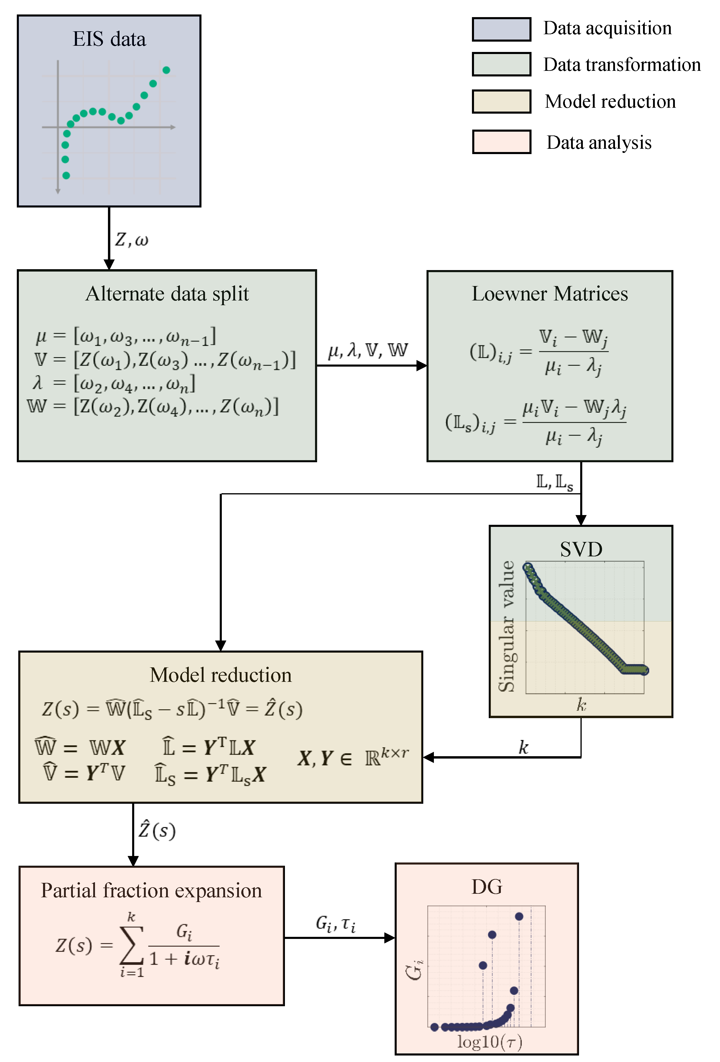
The work is structured as follows: Section 2 contemplates the mathematical and methodological approach of the LM. In Section 3 the LM is applied to different impedance data to determine the distribution of gains. Therefore, firstly, the DGs for different ECMs are determined and compared to their known time constants and gains. Afterwards, the impact of noise is investigated and, finally, an LIB is characterized through the approach. To verify the results, the distribution of gains obtained from the LM is compared to the gDRT in Section 4. Therefore, two impedance spectra, one at the begin of life (BOL) and one at the end of life (EOL), are analyzed. Finally, in Section 5, the results are summarized and suggestions for future work are given.

2. Loewner Method

Model order reduction usually refers to the sub-discipline of computing low-order dynamical systems of differential equations by means of numerical tools. Such models are required to approximate and preserve the properties and/or the structure of the original, potentially large-scale dynamical system.
However, in many engineering practices, the models expressed in the input–state–output framework are not exactly known, motivating the extension of the classical results to the data-driven model order reduction paradigm. Hence, analysis in the data-driven context is absolutely necessary. A purely-interpolatory, data-driven approach is the Loewner framework (LF) which was introduced in [28]. This can be used to learn/discover reduced-order dynamical models from frequency–response measurements, i.e., evaluations of the transfer function on a particular grid in the complex plane.
In this section, we present a short summary of the LF, as originally introduced in [28]. The main attribute of this data-driven approach is that it does not need any prior knowledge of the original hidden model, but only samples of the frequency response corresponding to it. Hence, without having access to the exact equations governing the original dynamics, LF reconstructs a surrogate model that matches well the input–output behavior of the hidden dynamical system. The reconstructed LF is subsequently extended by an eigenvalue decomposition to determine the gains and time constants of the underlying electrochemical processes of the impedance [30]. In this work, the entire evaluation process is described as the Loewner method. A procedure diagram of the whole process can be found in Figure 1.
For fairly extensive tutorial papers on LF for linear systems which tackle implementation issues and provide insights into many types of applications, we refer the reader to [33,34], as well as to the recent book on interpolation-based methods [35]. Furthermore, the problem of noisy/perturbed measurements was addressed in [36,37]. Finally, processing methods for identifying the polynomial terms in the transfer function from data were proposed in [38]. There, the behavior at is encoded by the presence of Jordan blocks in the system’s matrix pencil.
The LF is based on frequency–domain measurements { ( i ω , H ( i ω ) | 1 2 n } corresponding to the transfer function of the underlying unknown/hidden dynamical system, described in state–space representation by
E x ˙ ( t ) = A x ( t ) + B u ( t ) , y ( t ) = C x ( t ) + D u ( t ) .
We denote with N the order of the minimal linear dynamical system of equations in (1); there, x ( t ) R N is the state variable, u ( t ) is the control input, and y ( t ) is the observed output. Typically, in the LF, we do not have direct access to system matrices E , A R N × N , B , C T R N × 1 , or to D R . Instead, frequency response data are used, i.e., samples of the transfer function Z ( s ) = C ( s E A ) 1 B corresponding to system (1). Such data values can be inferred in various fields of engineering, from numberless types of practical experiments. The interpolation problem under hand is formulated as follows, given measured or computed data values partitioned into two disjoint subsets:
{ ( i ω , Z ( i ω ) | 1 2 n } right data : { λ j , Z ( λ j ) , j = 1 , , n } , and , left data : { μ i , Z ( μ i ) , i = 1 , , n }
Here, the λ j s and μ i s are selected from the measurement points i ω , typically in an alternate manner. We seek to find a low-order rational function H ^ ( s ) , corresponding to a reduced-order dynamical model, so that the following interpolation conditions hold:
Z ^ ( μ i ) = Z ( μ i ) : = v i , Z ^ ( λ j ) = Z ( λ j ) : = w j .
The first step is to re-arrange the data into matrix format; in this direction, let the Loewner matrix L C n × n and the shifted Loewner matrix L s C n × n be defined as follows:
L ( i , j ) = v i w j μ i λ j , L s ( i , j ) = μ i v i λ j w j μ i λ j ,
while the data vectors V C n × 1 , W C 1 × n are
V ( i , 1 ) = v i , W ( 1 , j ) = w j , for i , j = 1 , , k .
The raw, unprocessed LF model is composed of matrices
E ˜ = L , A ˜ = L s , B ˜ = V , C ˜ = W E ˜ x ˜ ˙ ( t ) = A ˜ x ˜ ( t ) + B ˜ u ( t ) , y ˜ ( t ) = C ˜ x ˜ ( t ) .
The data-driven state–space reconstructed model computed in (6) through the Loewner approach acts as a surrogate to the original linear model that generated the data, or as a faithful approximant thereof. The distinction will be clarified in the following paragraph.
In the case n = N , the original system in (1) is perfectly recovered. In case n < N we can compute merely an approximated model by means of interpolation, i.e., there are no guarantees that the information is fully recovered. If n > N , which is usually the case, we follow the compression procedure outlined below.
Consequently, in some practical applications characterized by large data sets, the matrix pair ( L s , L ) could be indeed singular, and hence, processing it may potentially cause numerical issues. This corresponds to the case k > n , i.e., “more data than necessary scenario”. In such scenarios, one needs to perform a singular value decomposition (SVD) of the Loewner matrices to extract the main/dominant characteristics, and to eliminate the inherent redundancies that cause the singularities to appear. Consequently, projection matrices X k , Y k C n × k are chosen as the left and, respectively, the right truncated singular vector matrices. More details can be found in [33]. Here, k N represents the truncation index and represents the order of the fitted model. When k = N , the original dynamics are perfectly recovered; however, a flexibility in choosing the value k is typically allowed in order to balance the accuracy of the fit and the complexity of the fitted model. The reduced-order Loewner matrices that contain the compressed data information are computed as follows:
L ^ = X k L Y k , L s ^ = X k L s Y k , V ^ = X k V , W ^ = W Y k .
The system matrices corresponding to a compressed LF of dimension k can be computed:
E ^ = L ^ , A ^ = L s ^ , B ^ = V ^ , C ^ = W ^ E ^ x ^ ˙ ( t ) = A ^ x ^ ( t ) + B ^ u ( t ) , y ^ ( t ) = C ^ x ^ ( t ) .
The transfer function of the fitted reduced-order model can be written as
Z ^ ( s ) = C ^ ( s E ^ A ^ ) 1 B ^ = W ^ ( L s ^ s L ^ ) 1 V ^ .
We now follow the procedure of the algorithm proposed in [29,30,32]. In order to extract time constants and gains from the matrices in (7), a generalized eigenvalue decomposition (EVD) of the matrix pair ( A r , E r ) needs to be performed:
L s ^ = L ^ V r Σ r V r 1 ,
with Σ r = diag ( λ 1 , , λ r ) C r × r as the matrix of eigenvalues, and V r = [ v 1 v 2 v r ] C r × r is the matrix of right eigenvectors. Let also V r 1 = [ v ˜ 1 v ˜ 2 v ˜ r ] C r × r . Then, in the case of invertible matrix E r , the transfer function in (9) is appropriately rewritten as
Z ^ ( s ) = W ^ ( L s ^ s L ^ ) 1 V ^ = W ^ ( s I r L ^ 1 L s ^ ) 1 ( L ^ 1 V ^ ) = W ^ ( s I r V r Σ r V r 1 ) 1 ( L ^ 1 V ^ ) = [ W ^ V r ] ( s I r Σ r ) 1 [ V r 1 L ^ 1 V ^ ] = i = 1 r r i s λ i .
The residues constitute the diagonal elements of the eigenvalues matrix Σ r , while the residues of transfer function Z r can be obtained by the following equation:
r i = [ W ^ v i ] [ v ˜ i T ( L ^ 1 V ^ ) ] .
Afterwards, the time constants and the poles can be computed by applying, respectively, the following formulas:
R i = r i λ i , τ i = 1 λ i , 1 i r ,
which transform Z r ( s ) = i = 1 r r i s λ i to Z r ( s ) = i = 1 r R i 1 + τ i s . More details are to be found in the flow chart from Figure 1, and in the original preceding publications [29,30].

3. Application of Loewner Method for Process Identification

The LM is applied to different ECMs in this section. This offers the possibility to compare the results with the known time constants of the assumed elements. At first, the SVD method is usedfor the determination of the model order as introduced in Section 2. The resulting model orders and DGs are analyzed and discussed in detail, as well as the influence of noise on the SVD , which is reviewed in Section 3.2. All calculations are performed on a Windows 11 home unit with an AMD Ryzen 5 Pro 4650U processor and 32 GB RAM using Matlab 2020b.

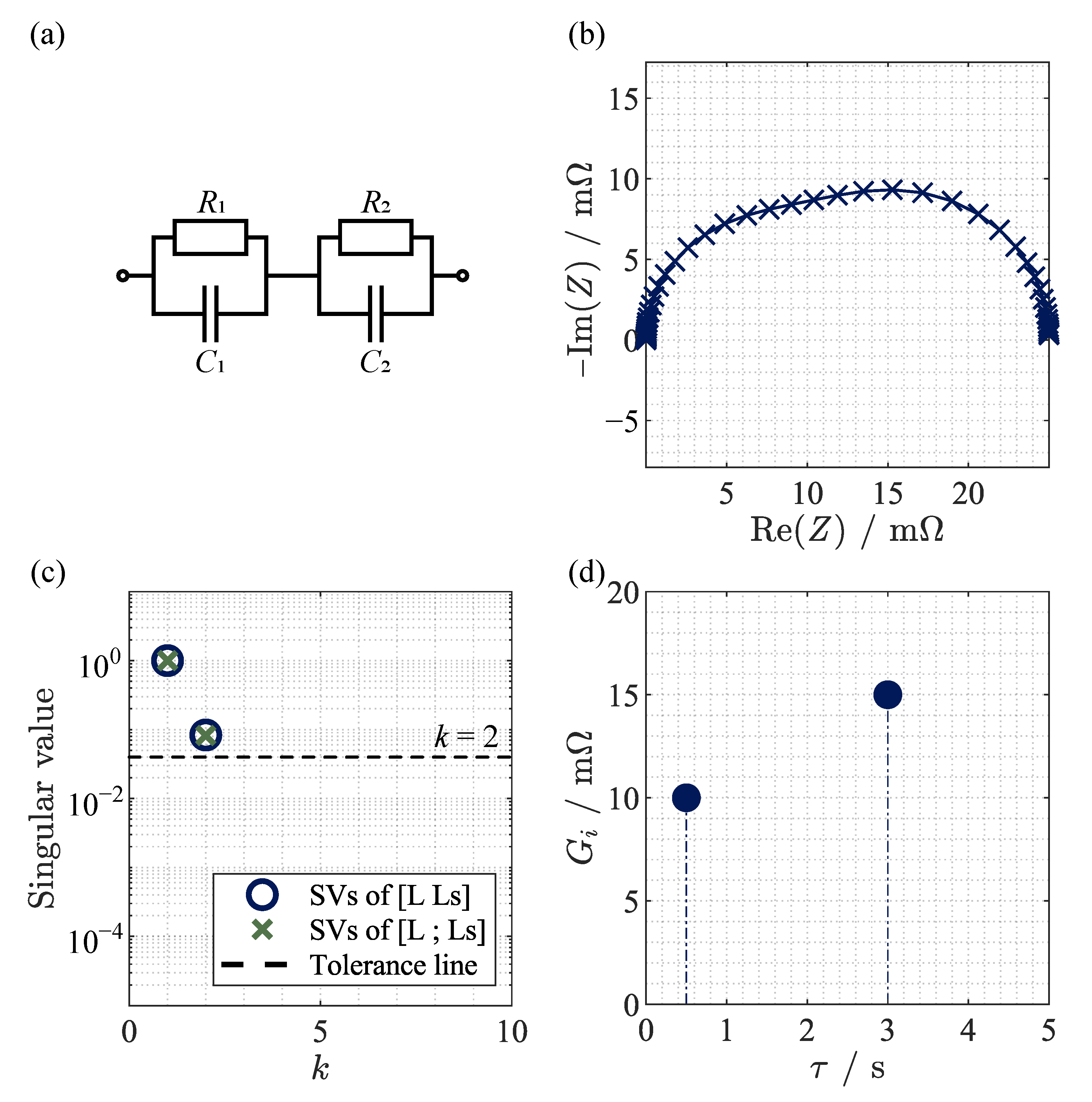
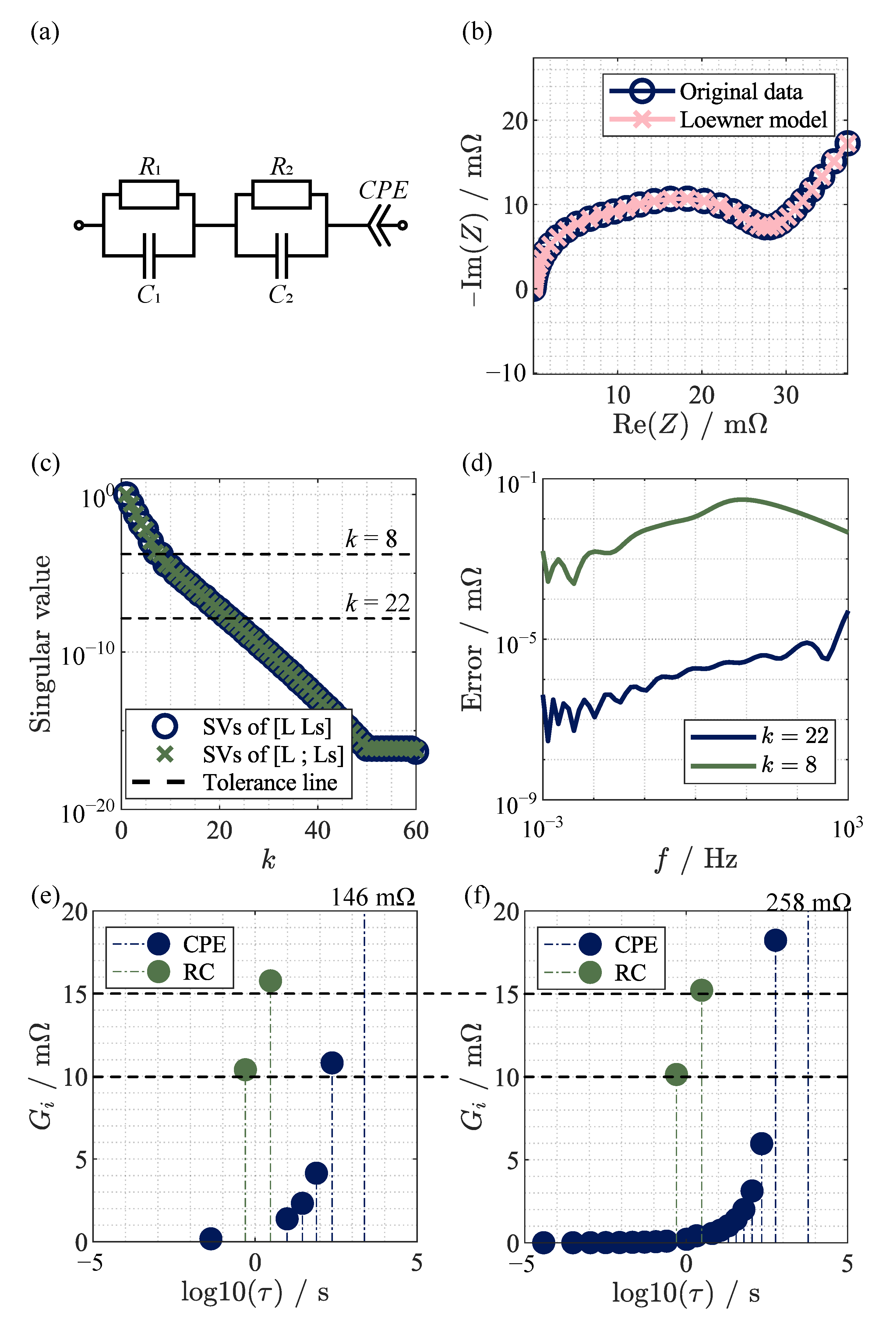
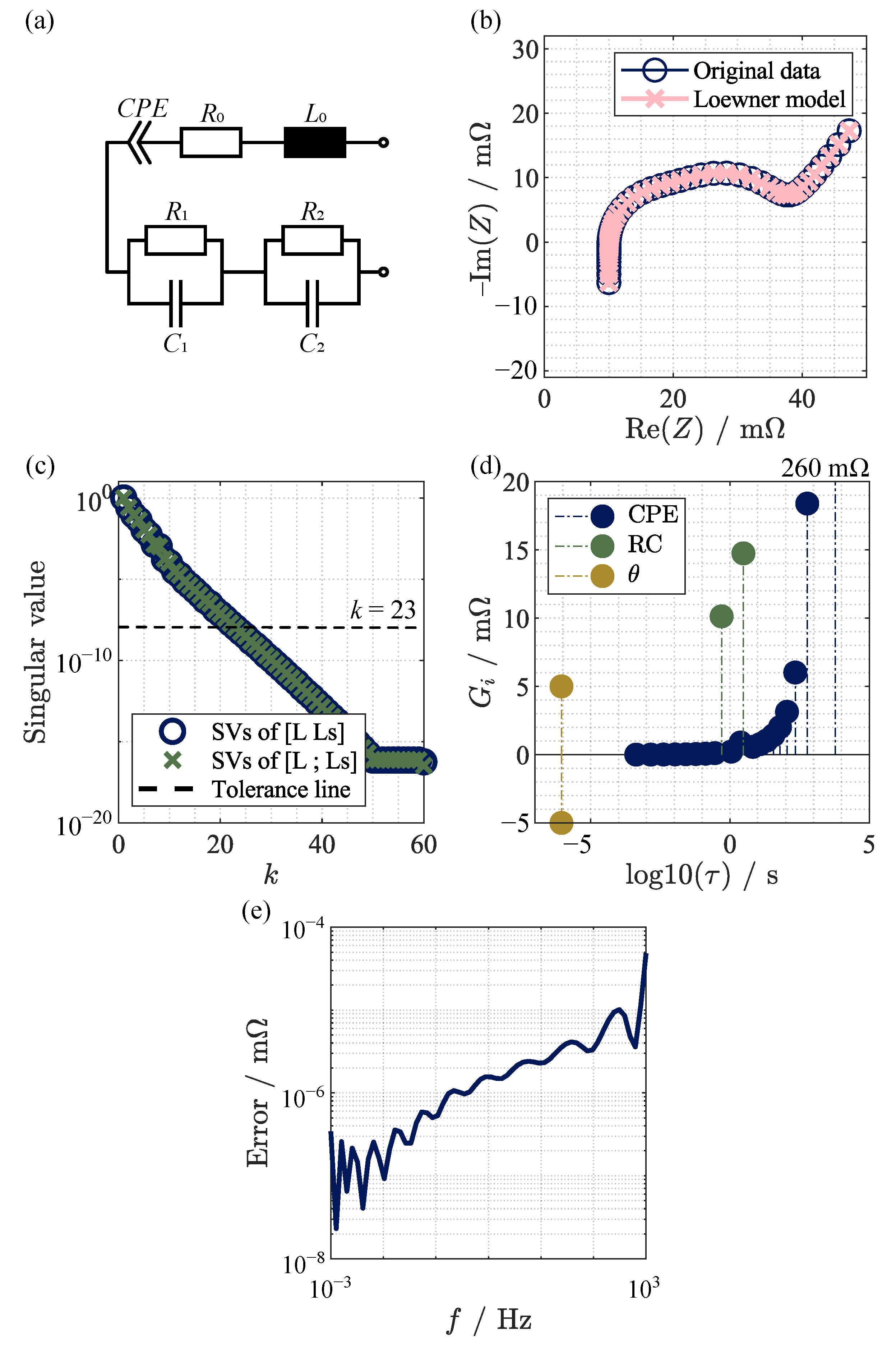
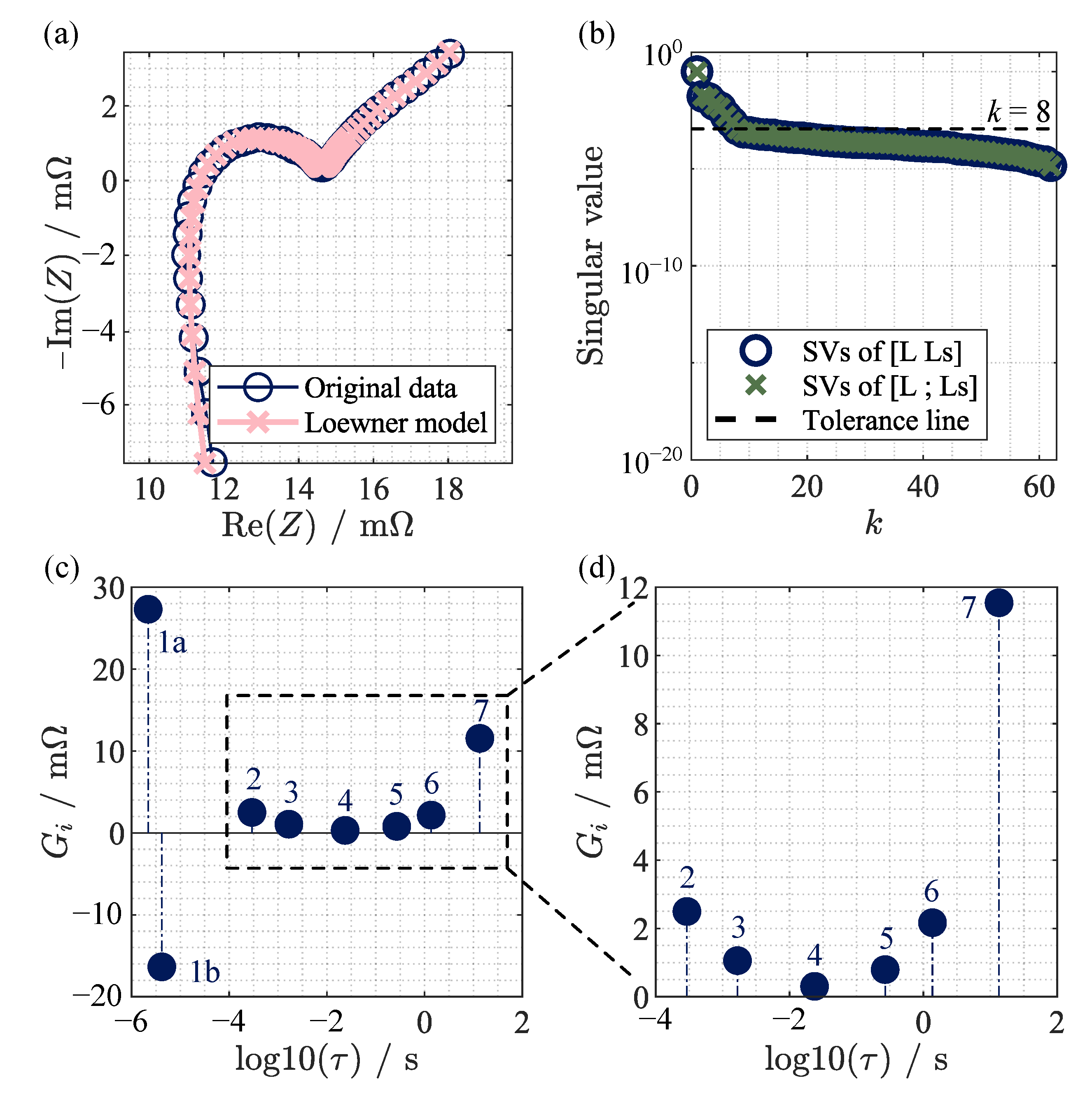
3.1. Analysis of Different Equivalent Circuit Models

The impedances used in this section are uniformly determined in a frequency range of 10 3 f 10 3 in a logarithmic distance with a total of 60 frequency points.
In the first ECM, two RC elements are connected in series, as shown in Figure 2a. The complex impedance Z RC is calculated through
Z RC = R 1 1 + i ω τ 1 + R 2 1 + i ω τ 2 ,
where R is the corresponding resistance of the RC element and τ = R C the time constant, taking the capacity C into account. The impedance is calculated for all frequency points, considering the angular frequency ω = 2 π f . The Nyquist plot of the resulting impedance spectrum for R 1 = 10 m Ω , R 2 = 15 m Ω , τ 2 =   0 , 5   s , and τ 1 = 3 s is shown in Figure 2b. It can be seen that in the superposition of the two semicircles the RC elements are difficult to separate.
As shown in Figure 2c, the SVD implies an existing model order of k = 2 , which fits to the order of Equation (14). Although singular values can be determined for higher model orders, these can be neglected since they have a magnitude of 10 17 and are therefore relegated to the numerical calculation.
The DG (Figure 2d) shows that the exact values of the time constants and gains can be recovered by employing the LM. Since the values in this simple example correspond exactly to the ECM diagram, no error analysis is performed.
However, RC elements represent only processes with a fixed time constant, so it is necessary to evaluate how the method behaves with distributed processes. For this reason, Sorrentino et al. [30] examined ZARC and Gerischer elements. However, those elements cannot directly represent the typical diffusion behavior of an LIB in the frequency domain. In the literature, a constant phase element (CPE) is often used to represent this characteristic low-frequency behavior [39,40]. Therefore, the previously investigated ECM is extended by a CPE, as shown in Figure 3a. The impedance
Z RC , CPE = R 1 1 + i ω τ 1 + R 2 1 + i ω τ 2 + 1 ( i ω ) ϕ C CPE ,
is expanded by the parameter C CPE = 1000 and the exponent ϕ = 0.6 . In the Nyquist plot (Figure 3b), the superposition of the RC elements and the CPE becomes visible. The low-frequency minimum and the diffusion branch arise through the model adaption, which are both characteristic features of LIBs.
The curve of the SVD in Figure 3c shows significantly different behaviour when considering elements with distributed time constants, offering three options for the choice of model order:
  • Using the bend point of the singular value curve, considering all values with the highest gradient, leading to k = 8 ;
  • Introducing a tolerance limit, here exemplary 10 8 leading to k = 22 ;
  • Choosing the first model order in which the singular values are (nearly) zero.
The last option will inevitably lead to over fitting due to the high arising model order. Furthermore, no zero values of the SVD occur for real measured data. For this reason the method is not further analyzed. The differences between the first two methods are discussed in detail below.
As can be seen in Figure 3d, a higher model order leads to a reduced error of the magnitude. However, the DG in Figure 3e,f shows that even for a lower model order, the qualitative course of the gains can be seen. The CPE element exhibits a continuously flattening progression from high time constants to low time constants. Thereby, at high time constants extremely high gains occur. This is attributed to the transfer function of the CPE, which cannot be determined directly with the partial fraction decomposition. In order to represent the behaviour of a CPE with the given Equation (3), the mentioned high values for high time constants are needed.
Furthermore, the DG shows a superposition of the RC elements and the CPE. The gains differ by 3.98 % and 5.15 % for k = 8 and 1.43 % and 1.45 % for k = 22 . Accordingly, the effect is reciprocal to the model order. The reason for this is that the peaks present at lower model order must cover a wider range of time constants. Another difference between the two cases is that the peak at the highest time constant increases significantly with the model order. This is attributed to the superposition of the individual peaks in combination with the impedance function of the CPE. At lower model order, the peak at the highest time constant must also cover other processes at lower time constants and is therefore limited in terms of its gain. With increasing model order, this effect will become less prominent and the gain of the peak is increased.
To illustrate the underlying effects in more detail, a video of the distribution of gains as a function of model order is included in the Supplementary part of this work. For the upcoming investigations, the tolerance method is chosen provided that a decent gradient of the singular values is present. If this is not the case (usually for measurement data), the method of the bend point is used.
Since purely resistive and inductive effects also need to be taken into account, the corresponding lumped elements are added to the ECM according to Figure 4a. Hence, the impedance is calculated through
Z Battery ( i ω ) = R 0 + i ω L 0 + R 1 1 + i ω τ 1 + R 2 1 + i ω τ 2 + 1 ( i ω ) ϕ Q CPE ,
considering the ohmic resistance R 0 = 10   m Ω and the inductance L 0 = 10   μ H . The resulting Nyquist plot, shown in Figure 4b, matches qualitatively to that of an LIB. The SVD pictured in Figure 4c no longer shows the characteristic first bend point but exhibits an almost constant gradient for a wide range of model orders. To allow fair comparison to the previous examined model, the tolerance value is chosen to be the same, resulting in a model order of k = 23 .
In the DG (Figure 4d), two peaks at 11 n s occur, which are assigned to the lumped elements since the polarization is quasi instantaneous. For clarity, these peaks are plotted as positive time constants with the corresponding gains. These peaks are represented in the partial fraction decomposition as Jordan blocks. This means that the time constant and the gain are complex values. Here, the amount of the real and imaginary part for both peaks are similar but differ in the sign of the imaginary part:
G Battery [ 5   m Ω i 556   m Ω , 5   m Ω + i 556   m Ω , ] ,
τ Battery [ 11   n s i 8.98   n s , 11   n s + i 8.98   n s , ] .
Consider the impedance function characterizing the behavior at of Z Battery ( i ω ) in (16) as Z ( i ω ) = R 0 + i ω L 0 . This polynomial of degree 1 can be realized by an order n = 2 DAE (differential-algebraic equation) system; a minimal realization can be written as
E = 0 1 0 0 , A = 1 0 0 1 , C = 1 0 , B = R 0 L 0 .
The dynamics are written as follows (here, x ( t ) = x 1 ( t ) x 2 ( t ) T ):
E x ˙ ( t ) = A x ( t ) + B u ( t ) , y ( t ) = C x ( t ) . x ˙ 2 ( t ) = x 1 ( t ) R 0 u ( t ) , 0 = x 2 ( t ) L 0 u ( t ) , y ( t ) = x 1 ( t ) .
It is to be noted that the second equation above, i.e., 0 = x 2 ( t ) L u ( t ) , is the algebraic condition (no dynamics, since the differential part is 0). Additionally, simple computations can confirm that
Z Battery ( i ω ) = C ( i ω E A ) 1 B = R 0 + i ω L 0 .
We note that E is a Jordan block with a double eigenvalue 0. Such matrices are very prone to perturbations, see [41]. By perturbing the entries of matrix E with ϵ > 0 , the 0 eigenvalues (time constants) will modify with a value of ϵ (in absolute value). This means that, for example, if ϵ = 10 12 , we actually perturb the time constants from a double 0 to ϵ ( 1 ± ı ı ˙ ) = 10 6 ( 1 ± ı ı ˙ ) . Additionally, such a Jordan block will be included in the large Loewner data matrix (before the compression step). After compression, the Jordan structure is most likely lost (because of numerical perturbations). It was shown in [38] that in order to preserve the Jordan structure (behavior at infinity), one needs to apply certain processing steps. Basically, these are needed to estimate the polynomial terms from data of the transfer function, i.e., R 0 and L 0 in (16) as a first step. Then, as a second step, the estimated polynomial part should be subtracted from the data, and the then classical Loewner approach can be applied to the processed data. Finally, the polynomial part is re-attached to the fitted (strictly-proper) transfer function to yield the required approximant.
However, the peaks associated with such Jordan blocks cannot be directly assigned to a lumped element. The sum of the two peaks is rather
θ = G 1 1 + i ω τ 1 + G 2 1 + i ω τ 2
a superposition of the resistance and the inductance. To determine the values of those lumped elements, the assumption
θ = R 0 + i ω L 0 ,
can be made. This requires that the peaks are not influenced by the effects of other elements (or processes), as will be further discussed in Section 3.3. Looking at the limit value consideration
lim ω 0 θ = R 0 = Re ( θ ) ,
it becomes clear that the real part of θ represents the pure ohmic part of the impedance. Consequently, the inductance L 0 can be determined by means of
L 0 = θ R 0 ω .
Pursuing this idea, a relative error of 0.03 % and 0.02 % can be determined for R 0 and L 0 , respectively. Therefore, this method can be used to determine the lumped elements.
Investigating the error of the magnitude in Figure 4e shows a progression over several orders of magnitude. In the low frequency range in which the CPE element has the highest polarization contribution, the largest deviations occur. As already described, these are due to the impedance function which cannot be represented precisely by means of the partial fraction decomposition due to the restricted model order. In the high frequency area the deviation becomes smaller, since the Jordan blocks offer an accurate method to display the inductive behavior. Comparing the error of the battery model with that of the model with two RC elements and CPE it can be seen that higher values arise. This is because the model order k for the DG has only been increased by one due to the SVD analysis. The model order of the impedance function on the other hand has increased by two. Furthermore, the superposition of the CPE and lumped elements, which the partial fraction decomposition cannot directly describe, has an impact on the deviation. However, the mean error remains in a low range with a value of 2.7 × 10 4 ‰.

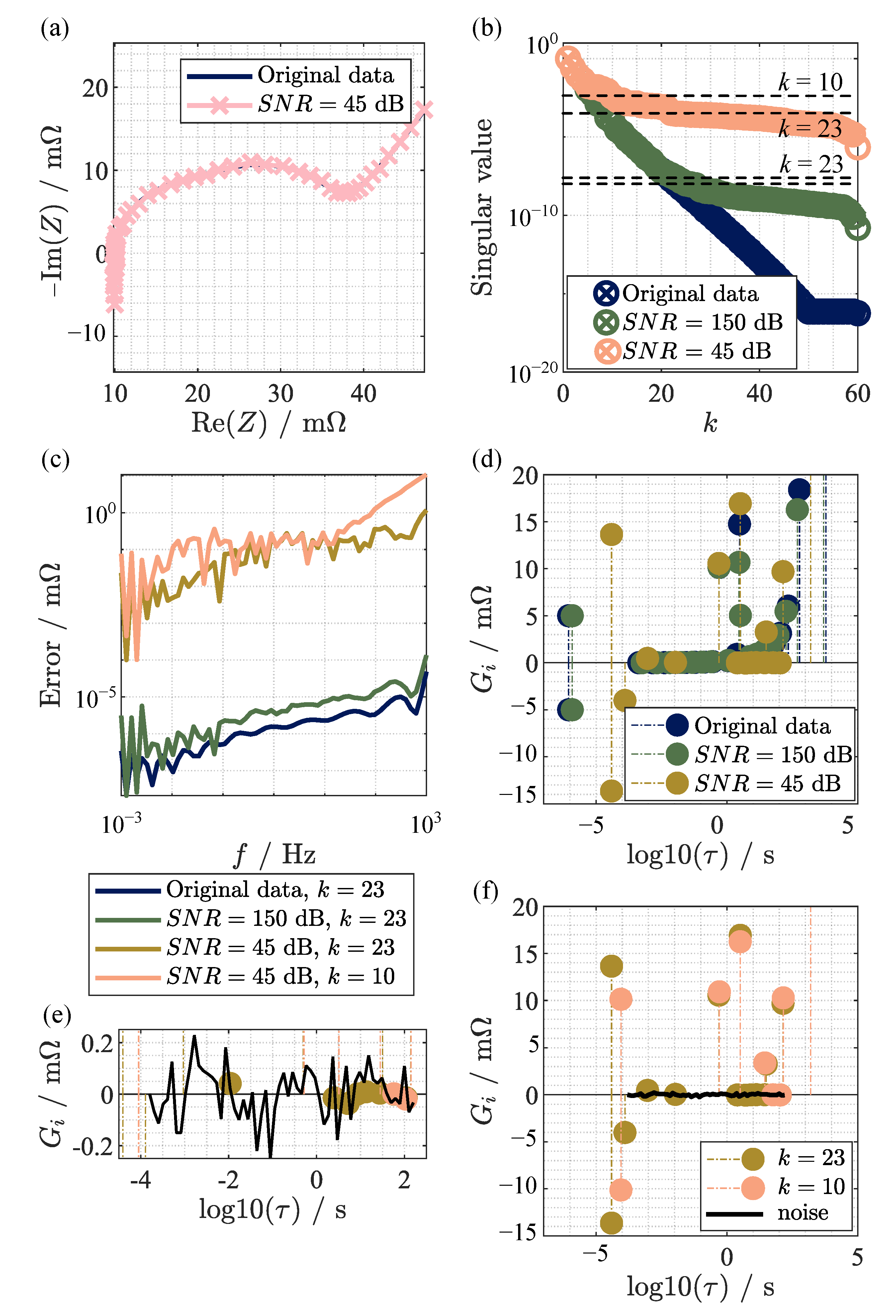
3.2. Analysis of Noise

To investigate the effect of measurement noise to the LM, complex valued white Gaussian noise was added to the impedance function (16) of the battery model. The model order was chosen in the same way as in Section 3.1 ( k = 23 ) to allow a fair comparison of the effects.
At first, a signal-to-noise ratio (SNR) of 150 was added to the impedance through the Matlab algorithm awgn. Since this small noise value leads to no visible deviations in the Nyquist plot, it is not shown separately. Nevertheless, these deviations already affect the singular values as shown in Figure 5b. The curve flattens significantly for higher model orders and shows a much higher minimal value. From Figure 5c, it is visible that there is a slight mean offset of about 5.8   μ Ω in magnitude between the original and S N R = 150 data. In the DG, those effects can be directly seen by three effects. The first is the shifting of time constants. Peaks at time constants below 62.4   s shift to higher values and peaks above this value shift to lower ones. The second effect is the slight change of gains, which is coupled with the shift of the time constants. The last effect is the split of the peak of the second RC element. Two new peaks are formed to the right and left of the original peak, which add up approximately to the magnitude of the original peak.
This effect becomes more clear when comparing the amplitude of noise with the DG according to Figure 5e. However, an investigation of the lower model order k displays only the peaks, which are due to the underlying processes. Choosing k = 10 through the previously mentioned bend point method results in the DG shown in Figure 5f. There, it can be seen that the number of peaks and the gains of the corresponding peaks differ. However, the characteristic course of the process-relevant peaks is still visible. The error of the magnitude underlines this behavior, as these deviate only slightly between the two model orders. Only at the lower frequency range do higher deviations occur, which are due to the fact that the CPE can only be represented to a certain extent by the lower model order.
In summary, it can be said that by applying noise, information about the underlying impedance function is lost. Therefore, choosing higher model orders is not recommended, since these partially represent the measurement noise. Using the bend point method as an indication for the model order has provided promising results. However, the proper determination of the model order remains a challenging task which must be carried out based on experience values.

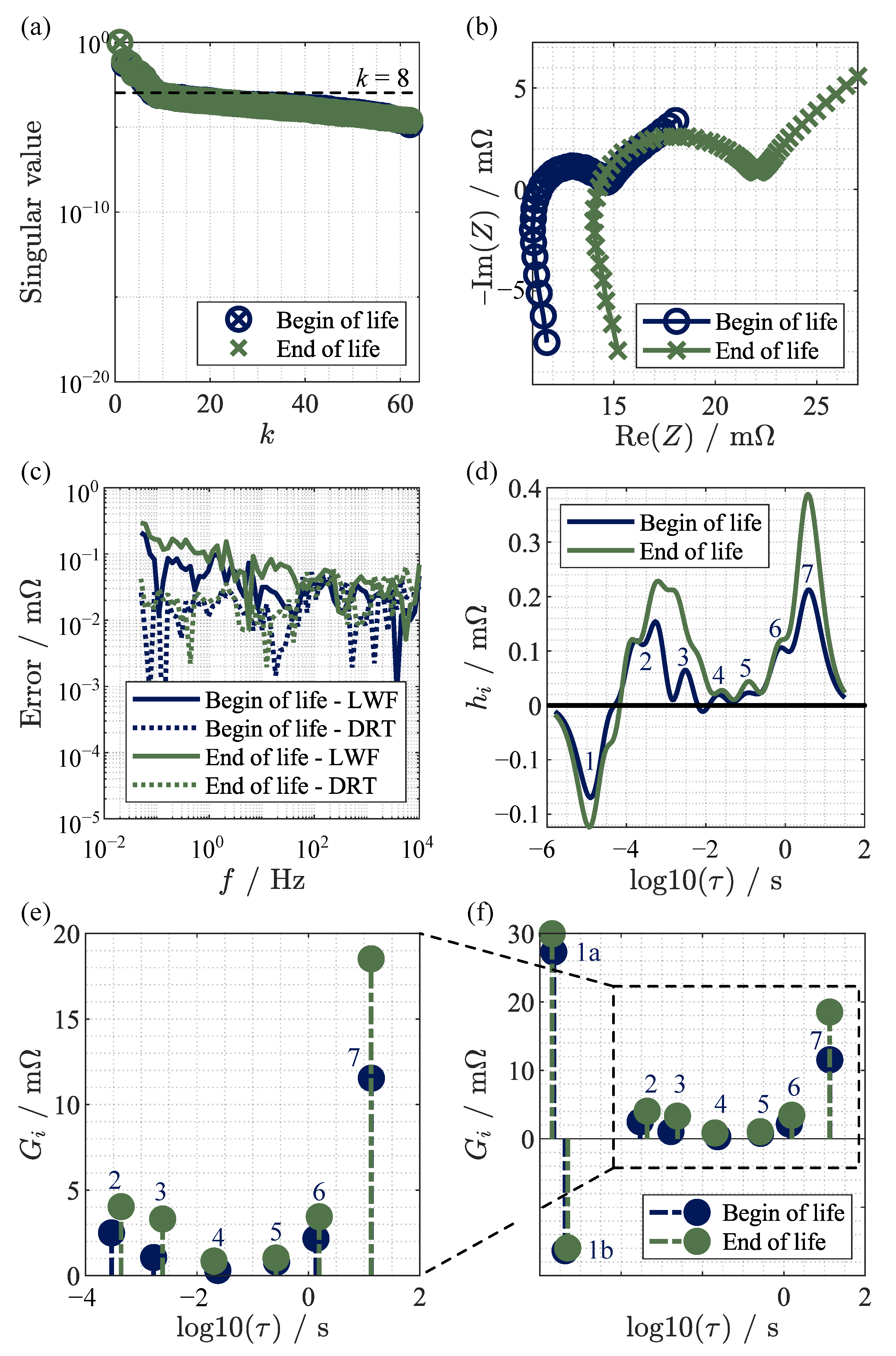
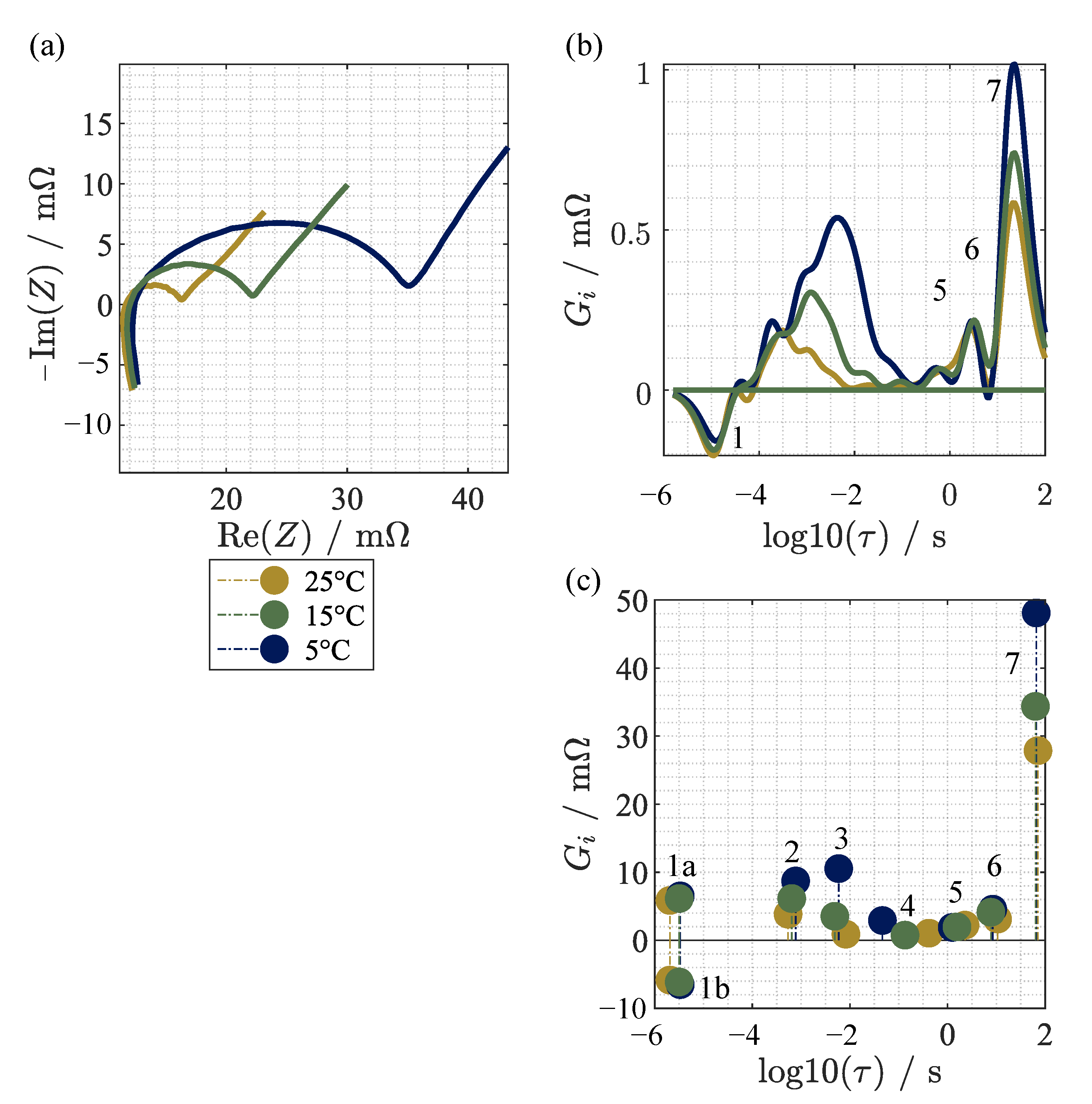
3.3. Measured Impedance Data

In a final step, the LM is applied to measured impedance spectra. The device under test is a cylindrical SAMSUNG INR21700-50E LIB with a nominal capacity of 4.9   A   h . The cell is charged to 50% and relaxed for multiple hours afterwards. The EIS is measured using a Zahner Zennium Pro. The measurements are conducted galvanostatically with an amplitude of 150   m A in a frequency range from 50   mHz to 10   kHz and validated with an extended Kramers–Kronig test according to Plank et al. [42]. The Nyquist plot of the resulting spectrum is shown in Figure 6a. The matching SVD is pictured in Figure 6b. Due to the noise in the measurement data, the perturbations of the SVD described in Section 3.2are apparent. The model order is therefore chosen through the bend point method leading to a model order of k = 8 . The DG that results from the measured impedance spectrum is plotted in Figure 6c. Clearly visible is a large inductive and resistive–inductive contribution at very low time constants. These are caused by the design of the cylindrical cell, where the rolled-up electrode sheets usually contribute largely to the inductive cell behavior. An apparent issue for the DG in this case is that due to the presence of inductive, resistive, and combined resistive–inductive behavior, the separation of those contributions is no longer possible. The peaks 1a and 1b, which are representative of this, are also no longer present as a Jordan block, since they differ in terms of time constants. It would therefore be necessary to determine the lumped elements prior for a comprehensive interpretation of the DG and determine the combined resistive–inductive behavior afterwards. Since this is less interesting for the analysis of the electrochemical cell behavior, it is neglected for further interpretation. A closer look is now taken at the processes at higher time constants with a close up of the distribution pictured in Figure 6d.
The remaining gains show a large contribution at high time constants which is usually assigned to the solid-state diffusion in the electrode particles. In the regime of time constants from 1 × 10 4 s to 1 s, the distribution shows five processes. The process with the lowest time constant lies in a regime that is too fast to be caused by charge transfer effects or the crossing of boundary layers. It can therefore be concluded that peak 2 is linked to electric effects such as particle–particle contact resistances or similar. The polarization contribution at peak 3 fits the dynamics of boundary layer crossing and is caused by the usually more dominant effects on the anode most likely linked to the anode’s solid electrolyte interphase (SEI). The three peaks between 1 × 10 2 s   s and 1 s   show dynamics that are often assigned to charge transfer of lithium ions. Whether the single gains are linked to charge transfer on the anode or cathode side can hardly be distinguished. To distinctively determine the electrochemical processes behind the polarization contributions visible in the distribution of gains, further measurements containing the variation of temperature and SOC is necessary, which is partly carried out in Section 4. Nevertheless, the polarization contributions, time constants, and number of processes that can be identified by the applied method are in very good agreement with process identification by EIS reported in the literature [22,43,44].

4. Comparison of Loewner Method and Generalized Distribution of Relaxation Times

To validate the results obtained from the LM, they are compared with the gDRT. For a detailed description and the mathematical background of the gDRT the reader is referred to Danzer [6]. Since the applied gDRT uses a Tikhonov regularization [6], its results are highly depending on the choice of its regularization parameter λ [19].There are several methods to determine this meta parameter [19,45,46,47]comprehensibly, but in this work the L-curve method introduced by Paul et al. [47] is used. The number of time constants n τ is chosen as three times the number of measuring points according to Hahn et al. [19].
First, the two methods are compared using the measurements introduced in Section 3.3 at the BOL of the cell. Afterwards, the cell was aged by cycling at 10   C with 1C in the CC phase for 20 cycles. With a total loss of about 19.9% of the initial capacity, the cell reached the initially defined EOL criterion. The capacity was measured during discharge using the CCCV method at a current of 0.5C and at 25 C . The cutoff current was set to 0.05C. Since the cell under test is a high-energy cell with a maximum continuous charging current of 0.5C specified in the data sheet, these are extraordinarily harsh fast charging conditions. Consequently, this let to a rapid decrease in available capacity. At this point, the impedance was measured similar to Section 3.3 and both results are compared. This comparison is of special interest since the ability of the LM to not simply describe the system under investigation but, beyond this, to enable a secure and easy track of the system’s behavior with changing parameters is investigated.
For the BOL measurement, it can be seen in Figure 7c that the mean error is 23.97   μ Ω lower for the gDRT. This is due to the significantly higher model order, which is 189 for the gDRT and 8 for the LM. By comparing the DG by the LM in Figure 7f and the DG by gDRT in Figure 7d, it is shownthat the peaks are located at approximately the same time constants and have the same qualitative course. However, for higher time constants, a mismatch can be found between the gDRT and LM. The reason for this is that both methods cannot represent the diffusion behavior directly. The regularization of the gDRT as well as the limited model order of the LM lead to the deviating results. Furthermore, process 2 of the gDRT shows multiple peaks, while the same process in the LM only shows a singular process in the middle of the time constants of the two peaks of the gDRT. The behavior of the gDRT could therefore be attributed to the combination of measurement noise in conjunction with regularization. The peaks 4 and 5 would not be analyzed if the distribution was analyzed by only the gDRT, due to the low polarization contribution. However, as discussed later, these peaks change due to aging and can therefore not be assigned to noise. Therefore the LM offers the possibility to analyze these polarization contributions. At low time constants of the gDRT, the inductive–resistive contribution occurs through peak 1. For the LM, it can be seen that the previous introduced θ splits up into the two peaks 1a and 1b, as discussed in Section 3.3 and Section 3.1. This can be attributed to the superposition of the inductive and inductive–resistive behavior. Since the inductive behavior is instantaneous, the peaks in the negative peak in the distribution of gains is shifted to lower time constants. The gDRT, however, only represents the resistive inductive part, since the pure inductive contributions are considered through a lumped element.
For the EOL measurement, the impedance shown in the Figure 7b arises. It is shifted by an ohmic offset and the half-circle width is extended. Investigating the SVD in Figure 7a reveals the same model order of k = 8 through the method of bend point. The mean difference between the error of the gDRT and the LM is with 5.1   μ Ω in the same order of magnitude as the BOL measurement. The comparison of the distribution of gains at BOL and EOL resulting from the LM is shown in Figure 7e,d. With the same same model order being optimal, the single polarization contributions can be clearly assigned to each other. The most apparent changes are visible for the peaks 2, 3, and 7. Peak 7, positioned at lower time constants, is usually attributed to solid-state diffusion. The growth of the gain at this peak is therefore a sign of worse diffusion processes in the electrode particles which is reported as a side effect of the reduced cell capacity [22]. The gains of the peaks 2 and 3 were attributed earlier to the crossing of boundary layers, such as the SEI by lithium ions. The larger contribution of these peaks to the cell polarization is most likely caused by the increased thickness of these boundary layers, either by further reaction between one of the electrodes and the electrolyte or by the metallic dissolution of metallic lithium on the anode. The latter is a common aging mechanism at low temperatures, high SOCs, and high charging currents [48], which matches the cycling parameters of the cell as well as the large capacity loss after only 20 cycles. Conclusively, the findings in the distribution of gains match the expected changes in the impedance of a cell that was strongly aged by metallic lithium deposition.
To further support the claims about the assignment of gains in the LM to electrochemical processes, two additional spectra taken at 15 C and 5 C are plotted in Figure A1 in the Appendix A. The DG accomplished by gDRT and LM both show a rising peak 7 with lower temperature, caused by the hindered solid-state diffusion at low temperatures. The bad low temperature performance of graphite is often attributed to rising charge transfer and SEI resistance in the literature [49,50,51]. Therefore, the rising polarization of peaks 2 and 3 at lower temperatures is a strong indication that these indeed show the crossing of boundary layers on the anode.
Comparatively, a more significant change in the resistive–inductive behavior is visible through gDRT, which cannot be separated from the change in purely resistive and inductive behavior by the LM. However, the allocation and separation of the individual processes is challenging in the gDRT, since the peaks change in terms of time constants and gains. Due to the regularization, a merge of peaks 2 and 3 occurs, which further challenges the interpretation of the results.
A quantitative comparison of the determined gains of the processes based on the two methods is not possible for two reasons. First, the gDRT, unlike the LM, provides a distribution of values for all processes rather than discrete values for individual processes. This leads to different magnitudes of the results. However, one could fit Gaussian peaks into the distribution function of the gDRT, as described in [19]. It remains questionable whether the assumption of this distribution function is correct. Moreover, the result of this peak fitting is subject to additional uncertainties due to the optimization algorithm used and the regularization of the gDRT. In Figure A2, it is shown that the number of peaks in the gDRT strongly depends on the regularization parameter. In addition, different regularization parameters can lead to the same number of peaks, resulting in different gains for the individual processes as can be seen in Table A2 for the BOL measurement. As mentioned earlier, identifying processes in EOL measurement with gDRT is challenging, further complicating the approach to quantification. Second, and probably more important, the two methods use distinctly different approaches to determine the results. Contrary to the LM, the gDRT does not consider the contribution of lumped elements (R, L, C) in the distribution of gains, but specifies these as additional values. Therefore, the values obtained by LM must be different to those of the gDRT at different time constants, which can be seen by comparing Table A1 and Table A2. Using the example of the polarization contribution of peak 7, it can be seen that the LM reaches higher values due to the capacitance considered. For this reason, only the previously conducted qualitative comparison of both methods is permissible.
Nevertheless, the interpretation of impedance data remains a difficult task that must be performed with care and by experts. Both the gDRT and the LM have different advantages and disadvantages which are summarized in Table 1. It can be concluded that neither method is superior and it may be beneficial to combine them in the future.

5. Conclusions

In this study, the Loewner method is introduced to determine the distribution of gains for the data-driven analysis and process identification of impedance spectra. The method is based on the model reduction by the Loewner framework, which is extended by an interpretation of the diagonal elements of the eigenvalue matrix.
In a first step, the method is verified using equivalent circuit models with known time constants and gains. Therefore, elements with fixed time constants (RC elements), distributed time constants (CPE), and lumped elements (R, L) are analyzed. Two challenges arise: the correct choice of the model order and the interpretation of lumped elements. For the first challenge, the bend point, tolerance limit, and zero singular value decomposition methods are examined. The results show that the tolerance method seems to be the most suitable for synthetic data, whereas for noisy data the bend point method seems to be advantageous. When interpreting the lumped elements, it is found that they are represented as Jordan blocks in the distribution of gains. With this knowledge, a method for determining the values of the lumped elements is developed and a deviation of 0.03% and 0.02% to the predefined values is obtained for the resistance and inductance, respectively. However, this method is only applicable to synthetic data containing resistive and inductive contributions only.
In a second step, the effects of the measurement noise are investigated. Already, a high signal-to-noise ratio leads to a significant change of the singular value decomposition which influences the choice of the model order. It is shown that analysis using the bending point method remains stable even under the influence of higher amplitudes of the measurement noise. Furthermore, it is found that the model order can be drastically reduced as the signal-to-noise ratio decreases without increasing the model error. The reason for this is the superposition of measurement noise and small polarization contributions.
In the third part of the study, the Loewner method is applied to measure impedance data of a cylindrical lithium-ion battery at two different states of health. The resulting distribution of gains is compared with the results obtained from the generalized distribution of relaxation times. Both methods show the same qualitative trajectories in the distribution function, with minor differences in error. It is found that process identification is easier with the Loewner method, since no peak fit needs to be conducted. In addition, aging effects are easier to assign since there is no overlap of peaks due to regularization as there are within the distribution of relaxation time analysis. This also leads to the effect that peaks with smaller gains can be evaluated. On the other hand, the interpretation of the lumped elements is challenging with this approach. For this purpose, the generalized distribution of relaxation times provides favorable behavior. In future work, both methods will be combined to overcome the disadvantages of each method. In addition, similar methods will be applied to time–domain data from lithium-ion batteries.
In summary, the Loewner method is an alternative, data-driven, and regularization-free approach for evaluating and analyzing impedance spectra from lithium-ion batteries as well as for the process identification of electrochemical storage and conversion systems.

Supplementary Materials

The following are available online at https://www.mdpi.com/article/10.3390/batteries9020132/s1.

Author Contributions

Conceptualization, T.R., I.V.G., A.C.A. and M.A.D.; methodology, T.R. and I.V.G.; software, I.V.G. and A.C.A.; validation, T.R. and L.J.; formal analysis, T.R., I.V.G. and L.J.; investigation, T.R., I.V.G. and L.J.; data curation, T.R. and L.J.; writing—original draft preparation, T.R., I.V.G. and L.J.; writing—review and editing, T.R., I.V.G., L.J., A.C.A. and M.A.D.; visualization, T.R.; supervision, A.C.A. and M.A.D. All authors have read and agreed to the published version of the manuscript.

Funding

This paper evolved from the research project ReDesign (Development of design guidelines for the recycling-oriented design of battery systems in context of the circular economy) which is funded by the Federal Ministry of Education and Research under grant number 03XP0318C. ReDesign is a part of the greenBatt cluster.

Data Availability Statement

Data available on request.

Conflicts of Interest

The authors declare no conflict of interest.

Abbreviations

The following abbreviations are used in this manuscript:
BOLBegin of life
CPEConstant phase element
DRTDistribution of relaxation times
ECMEquivalent circuit model
EISElectrochemical impedance spectroscopy
EOLEnd of life
gDRTGeneralized distribution of relaxation times
LIBLithium-ion battery
LMLoewner method
LWFLoewner framework
PEMFCPolymer electrolyte membrane fuel cell
SEISolid electrolyte interphase
SNRSignal-to-noise ratio
SOCState of charge
SVDSingular value decomposition

Appendix A

Figure A1. Nyquist plot (a), distribution of gains obtained by gDRT (b), distribution of gains obtained by LWF (c) of the measurement data at different temperatures.
Batteries 09 00132 g0a1
Figure A2. Number of peaks of the distribution of gains determined with gDRT as function of the regularization parameter.
Batteries 09 00132 g0a2
Table A1. Distribution of gains for the different processes obtained by LM.
1a 1b 2 3 4 5 6 7
BOL 27.30   m Ω 16.36   m Ω 2.50   m Ω 1.06   m Ω 0.30   m Ω 0.79   m Ω 2.17   m Ω 11.54   m Ω
EOL 29.96   m Ω 15.95   m Ω 4.03   m Ω 3.31   m Ω 0.85   m Ω 1.03   m Ω 3.44   m Ω 18.52   m Ω
Table A2. Distribution of gains for the different processes of the BOL measurement obtained by gDRT.
λ I II III IV V VI VII
0.08 3.58   m Ω 3.38   m Ω 0.67   m Ω 0.21   m Ω 1.46   m Ω 1.27   m Ω 3.65   m Ω
0.11 3.13   m Ω 3.38   m Ω 0.62   m Ω 0.20   m Ω 1.32   m Ω 1.22   m Ω 3.54   m Ω
0.14 2.99 m Ω 3.41   m Ω 0.60   m Ω 0.19   m Ω 1.19   m Ω 1.40   m Ω 3.28   m Ω

References

  1. Rodat, S.; Sailler, S.; Druart, F.; Thivel, P.X.; Bultel, Y.; Ozil, P. EIS measurements in the diagnosis of the environment within a PEMFC stack. J. Appl. Electrochem. 2009, 40, 911–920. [Google Scholar] [CrossRef]
  2. Fang, Q.; de Haart, U.; Schäfer, D.; Thaler, F.; Rangel-Hernandez, V.; Peters, R.; Blum, L. Degradation Analysis of an SOFC Short Stack Subject to 10,000 h of Operation. J. Electrochem. Soc. 2020, 167, 144508. [Google Scholar] [CrossRef]
  3. Middlemiss, L.A.; Rennie, A.J.; Sayers, R.; West, A.R. Characterisation of batteries by electrochemical impedance spectroscopy. Energy Rep. 2020, 6, 232–241. [Google Scholar] [CrossRef]
  4. Maheshwari, A.; Heck, M.; Santarelli, M. Cycle aging studies of lithium nickel manganese cobalt oxide-based batteries using electrochemical impedance spectroscopy. Electrochim. Acta 2018, 273, 335–348. [Google Scholar] [CrossRef]
  5. Katzer, F.; Rüther, T.; Plank, C.; Roth, F.; Danzer, M.A. Analyses of polarisation effects and operando detection of lithium deposition in experimental half- and commercial full-cells. Electrochim. Acta 2022, 436, 141401. [Google Scholar] [CrossRef]
  6. Danzer, M.A. Generalized Distribution of Relaxation Times Analysis for the Characterization of Impedance Spectra. Batteries 2019, 5, 53. [Google Scholar] [CrossRef]
  7. Yoo, H.D.; Jang, J.H.; Ryu, J.H.; Park, Y.; Oh, S.M. Impedance analysis of porous carbon electrodes to predict rate capability of electric double-layer capacitors. J. Power Sources 2014, 267, 411–420. [Google Scholar] [CrossRef]
  8. Schmidt, J.P.; Arnold, S.; Loges, A.; Werner, D.; Wetzel, T.; Ivers-Tiffée, E. Measurement of the internal cell temperature via impedance: Evaluation and application of a new method. J. Power Sources 2013, 243, 110–117. [Google Scholar] [CrossRef]
  9. McGrogan, F.P.; Bishop, S.R.; Chiang, Y.M.; van Vliet, K.J. Connecting Particle Fracture with Electrochemical Impedance in LiXMn2O4. J. Electrochem. Soc. 2017, 164, A3709–A3717. [Google Scholar] [CrossRef]
  10. Meddings, N.; Heinrich, M.; Overney, F.; Lee, J.S.; Ruiz, V.; Napolitano, E.; Seitz, S.; Hinds, G.; Raccichini, R.; Gaberšček, M.; et al. Application of electrochemical impedance spectroscopy to commercial Li-ion cells: A review. J. Power Sources 2020, 480, 228742. [Google Scholar] [CrossRef]
  11. Rüther, T.; Plank, C.; Schamel, M.; Danzer, M.A. Detection of inhomogeneities in serially connected lithium-ion batteries. Appl. Energy 2023, 332, 120514. [Google Scholar] [CrossRef]
  12. Carthy, K.M.; Gullapalli, H.; Ryan, K.M.; Kennedy, T. Review—Use of Impedance Spectroscopy for the Estimation of Li-ion Battery State of Charge, State of Health and Internal Temperature. J. Electrochem. Soc. 2021, 168, 080517. [Google Scholar] [CrossRef]
  13. Rivera-Barrera, J.; Muñoz-Galeano, N.; Sarmiento-Maldonado, H. SoC Estimation for Lithium-ion Batteries: Review and Future Challenges. Electronics 2017, 6, 102. [Google Scholar] [CrossRef]
  14. Galeotti, M.; Cinà, L.; Giammanco, C.; Cordiner, S.; Carlo, A.D. Performance analysis and SOH (state of health) evaluation of lithium polymer batteries through electrochemical impedance spectroscopy. Energy 2015, 89, 678–686. [Google Scholar] [CrossRef]
  15. Pan, Y.; Ren, D.; Han, X.; Lu, L.; Ouyang, M. Lithium Plating Detection Based on Electrochemical Impedance and Internal Resistance Analyses. Batteries 2022, 8, 206. [Google Scholar] [CrossRef]
  16. Schmidt, J.P.; Adam, A.; Wandt, J. Time-Resolved and Robust Lithium Plating Detection for Automotive Lithium-Ion Cells with the Potential for Vehicle Application. Batteries 2023, 9, 97. [Google Scholar] [CrossRef]
  17. Koseoglou, M.; Tsioumas, E.; Ferentinou, D.; Jabbour, N.; Papagiannis, D.; Mademlis, C. Lithium plating detection using dynamic electrochemical impedance spectroscopy in lithium-ion batteries. J. Power Sources 2021, 512, 230508. [Google Scholar] [CrossRef]
  18. Gaddam, R.R.; Katzenmeier, L.; Lamprecht, X.; Bandarenka, A.S. Review on physical impedance models in modern battery research. Phys. Chem. Chem. Phys. 2021, 23, 12926–12944. [Google Scholar] [CrossRef]
  19. Hahn, M.; Schindler, S.; Triebs, L.C.; Danzer, M.A. Optimized Process Parameters for a Reproducible Distribution of Relaxation Times Analysis of Electrochemical Systems. Batteries 2019, 5, 43. [Google Scholar] [CrossRef]
  20. Zhao, Y.; Kücher, S.; Jossen, A. Investigation of the diffusion phenomena in lithium-ion batteries with distribution of relaxation times. Electrochim. Acta 2022, 432, 141174. [Google Scholar] [CrossRef]
  21. Zhang, Q.; Wang, D.; Schaltz, E.; Stroe, D.I.; Gismero, A.; Yang, B. Degradation mechanism analysis and State-of-Health estimation for lithium-ion batteries based on distribution of relaxation times. J. Energy Storage 2022, 55, 105386. [Google Scholar] [CrossRef]
  22. Iurilli, P.; Brivio, C.; Wood, V. Detection of Lithium-Ion Cells’ Degradation through Deconvolution of Electrochemical Impedance Spectroscopy with Distribution of Relaxation Time. Energy Technol. 2022, 10, 2200547. [Google Scholar] [CrossRef]
  23. He, R.; He, Y.; Xie, W.; Guo, B.; Yang, S. Comparative analysis for commercial li-ion batteries degradation using the distribution of relaxation time method based on electrochemical impedance spectroscopy. Energy 2023, 263, 125972. [Google Scholar] [CrossRef]
  24. Illig, J.; Ender, M.; Weber, A.; Ivers-Tiffée, E. Modeling graphite anodes with serial and transmission line models. J. Power Sources 2015, 282, 335–347. [Google Scholar] [CrossRef]
  25. Chen, X.; Li, L.; Liu, M.; Huang, T.; Yu, A. Detection of lithium plating in lithium-ion batteries by distribution of relaxation times. J. Power Sources 2021, 496, 229867. [Google Scholar] [CrossRef]
  26. Brown, D.E.; McShane, E.J.; Konz, Z.M.; Knudsen, K.B.; McCloskey, B.D. Detecting onset of lithium plating during fast charging of Li-ion batteries using operando electrochemical impedance spectroscopy. Cell Rep. Phys. Sci. 2021, 2, 100589. [Google Scholar] [CrossRef]
  27. Bergmann, T.G.; Schlüter, N. Introducing Alternative Algorithms for the Determination of the Distribution of Relaxation Times. ChemPhysChem 2022, 23, e202200012. [Google Scholar] [CrossRef]
  28. Mayo, A.J.; Antoulas, A.C. A framework for the solution of the generalized realization problem. Linear Algebra Its Appl. 2007, 425, 634–662. [Google Scholar] [CrossRef]
  29. Patel, B. Application of Loewner Framework for Data-Driven Modeling and Diagnosis of Polymer Electrolyte Membrane Fuel Cells. Master’s Thesis, Otto von Guericke-University, Magdeburg, Germany, 2021. [Google Scholar]
  30. Sorrentino, A.; Gosea, I.V.; Patel, B.; Antoulas, A.C.; Vidakovic-Koch, T. Loewner Framework and Distribution of Relaxation Times of Electrochemical Systems: Solving Issues Through a Data-Driven Modeling Approach. SSRN Electron. J. 2022. [Google Scholar] [CrossRef]
  31. Gosea, I.V.; Zivkovic, L.; Karachalios, D.S.; Antoulas, A.C.; Vidakovic-Koch, T. A data-based nonlinear frequency response approach based on the Loewner framework: Preliminary analysis. In Proceedings of the 12th IFAC Symposium on Nonlinear Control Systems, Canberra, Australia, 4–6 January 2023; Elsevier: Amsterdam, The Netherlands, 2023. [Google Scholar]
  32. Sorrentino, A.; Gosea, I.V.; Patel, B.; Antoulas, A.C.; Vidakovic-Koch, T. The Loewner Framework for Data-Driven Identification of Electrochemical Systems; MPI: Magdeburg, Germany, 2022. [Google Scholar]
  33. Antoulas, A.C.; Lefteriu, S.; Ionita, A.C. A tutorial introduction to the Loewner framework for model reduction; Computational Science & Engineering, Society for Industrial and Applied Mathematics: Philadelphia, PA, USA, 2017. [Google Scholar]
  34. Gosea, I.V.; Poussot-Vassal, C.; Antoulas, A.C. Chapter 15: Data-driven modeling and control of large-scale dynamical systems in the Loewner framework: Methodology and applications. In Handbook of Numerical Analysis, Numerical Control: Part A; Trélat, E., Zuazua, E., Eds.; Elsevier: Amsterdam, The Netherlands, 2022; Volume 23, pp. 499–530. [Google Scholar] [CrossRef]
  35. Antoulas, A.C.; Beattie, C.A.; Gugercin, S. Interpolatory Methods for Model Reduction; Computational Science & Engineering, Society for Industrial and Applied Mathematics: Philadelphia, PA, USA, 2020. [Google Scholar]
  36. Embree, M.; Ionita, A.C. Pseudospectra of Loewner matrix pencils. In Realization and Model Reduction of Dynamical Systems; Springer: Berlin/Heidelberg, Germany, 2022; pp. 59–78. [Google Scholar] [CrossRef]
  37. Drmač, Z.; Peherstorfer, B. Learning low-dimensional dynamical-system models from noisy frequency-response data with Loewner rational interpolation. In Realization and Model Reduction of Dynamical Systems; Springer: Berlin/Heidelberg, Germany, 2022; pp. 39–57. [Google Scholar]
  38. Gosea, I.V.; Zhang, Q.; Antoulas, A.C. Preserving the DAE structure in the Loewner model reduction and identification framework. Adv. Comput. Math. 2020, 46, 1–32. [Google Scholar] [CrossRef]
  39. Wang, X.; Wei, X.; Zhu, J.; Dai, H.; Zheng, Y.; Xu, X.; Chen, Q. A review of modeling, acquisition, and application of lithium-ion battery impedance for onboard battery management. eTransportation 2021, 7, 100093. [Google Scholar] [CrossRef]
  40. Deng, Z.; Zhang, Z.; Lai, Y.; Liu, J.; Li, J.; Liu, Y. Electrochemical Impedance Spectroscopy Study of a Lithium/Sulfur Battery: Modeling and Analysis of Capacity Fading. J. Electrochem. Soc. 2013, 160, A553–A558. [Google Scholar] [CrossRef]
  41. Golub, G.H.; Van Loan, C.F. Matrix Computations, 3rd ed.; Johns Hopkins University Press: Baltimore, MD, USA, 1996. [Google Scholar]
  42. Plank, C.; Ruther, T.; Danzer, M.A. Detection of Non-Linearity and Non-Stationarity in Impedance Spectra using an Extended Kramers-Kronig Test without Overfitting. In Proceedings of the 2022 International Workshop on Impedance Spectroscopy (IWIS), Chemnitz, Germany, 27–30 September 2022. [Google Scholar] [CrossRef]
  43. Shafiei Sabet, P.; Sauer, D.U. Separation of predominant processes in electrochemical impedance spectra of lithium-ion batteries with nickel-manganese-cobalt cathodes. J. Power Sources 2019, 425, 121–129. [Google Scholar] [CrossRef]
  44. Manikandan, B.; Ramar, V.; Yap, C.; Balaya, P. Investigation of physico-chemical processes in lithium-ion batteries by deconvolution of electrochemical impedance spectra. J. Power Sources 2017, 361, 300–309. [Google Scholar] [CrossRef]
  45. Schlüter, N.; Ernst, S.; Schröder, U. Finding the Optimal Regularization Parameter in Distribution of Relaxation Times Analysis. ChemElectroChem 2019, 6, 6027–6037. [Google Scholar] [CrossRef]
  46. Schlüter, N.; Ernst, S.; Schröder, U. Direct Access to the Optimal Regularization Parameter in Distribution of Relaxation Times Analysis. ChemElectroChem 2020, 7, 3445–3458. [Google Scholar] [CrossRef]
  47. Paul, T.; Chi, P.W.; Wu, P.M.; Wu, M.K. Computation of distribution of relaxation times by Tikhonov regularization for Li ion batteries: Usage of L-curve method. Sci. Rep. 2021, 11, 12624. [Google Scholar] [CrossRef]
  48. Hu, D.; Chen, L.; Tian, J.; Su, Y.; Li, N.; Chen, G.; Hu, Y.; Dou, Y.; Chen, S.; Wu, F. Research Progress of Lithium Plating on Graphite Anode in Lithium–Ion Batteries. Chin. J. Chem. 2020, 39, 165–173. [Google Scholar] [CrossRef]
  49. Wang, C.; Appleby, A.J.; Little, F.E. Low-Temperature Characterization of Lithium-Ion Carbon Anodes via Microperturbation Measurement. J. Electrochem. Soc. 2002, 149, A754–A760. [Google Scholar] [CrossRef]
  50. Zhang, S.; Xu, K.; Jow, T. Low temperature performance of graphite electrode in Li-ion cells. Electrochim. Acta 2002, 48, 241–246. [Google Scholar] [CrossRef]
  51. Jow, T.R.; Delp, S.A.; Allen, J.L.; Jones, J.P.; Smart, M.C. Factors Limiting Li+ Charge Transfer Kinetics in Li-Ion Batteries. J. Electrochem. Soc. 2018, 165, A361–A367. [Google Scholar] [CrossRef]
Figure 1. Flow chart of the LM.
Batteries 09 00132 g001
Figure 2. ECM for two RC elements (a), Nyquist plot of the impedance Z RC (b), SVD of the Loewner matrices (c), DG (d).
Batteries 09 00132 g002
Figure 3. ECM for two RC elements and CPE (a), Nyquist plot of the impedance Z RC , CPE and LM with k = 22 (b), SVD of the Loewner matrices (c), error of magnitude for different model orders (d), DG for k = 8 (e) and k = 22 (f).
Batteries 09 00132 g003
Figure 4. ECM for battery model (a), Nyquist plot of the impedance Z Battery (b), SVD of the Loewner matrices (c), DG (d), and error of magnitude (e).
Batteries 09 00132 g004
Figure 5. Nyquist plot (a), SVD (b), error of magnitude (c), distribution of gains (d) for different level of noise. Distribution of gains for S N R = 45 for different model orders (e), zoom for the different model orders (f).
Batteries 09 00132 g005
Figure 6. Nyquist plot (a), SVD (b), distribution of gains (d), and analyzed processes of the distribution of gains (c) of the measurement data.
Batteries 09 00132 g006
Figure 7. SVD (a), Nyquist plot (b), error of magnitude (c), DG (d), zoom of the distribution of gains (e), distribution of gains (f) for the BOL and EOL LIB.
Batteries 09 00132 g007
Table 1. Advantages and disadvantages of LM and gDRT.
Lowener MethodGeneralized DRT
− Meta parameter needed (k)− Meta parameter needed ( λ , n τ )
+ Simple process identification− Difficult process identification
− Interpretation of resistive, capacitive, and resistive–inductive processes is challenging+ Interpretation of resistive, inductive, and resistive–inductive behavior possible
+ Smaller polarization contributions interpretable− Partial merging of peaks due to regularization
Disclaimer/Publisher’s Note: The statements, opinions and data contained in all publications are solely those of the individual author(s) and contributor(s) and not of MDPI and/or the editor(s). MDPI and/or the editor(s) disclaim responsibility for any injury to people or property resulting from any ideas, methods, instructions or products referred to in the content.

