Article

An Enhanced Single-Particle Model Using a Physics-Informed Neural Network Considering Electrolyte Dynamics for Lithium-Ion Batteries

1
School of Automotive Studies, Tongji University, Shanghai 201804, China
2
Clean Energy Automotive Engineering Center, Tongji University, Shanghai 201804, China
*
Authors to whom correspondence should be addressed.
Batteries 2023, 9(10), 511; https://doi.org/10.3390/batteries9100511
Submission received: 15 September 2023 / Revised: 13 October 2023 / Accepted: 13 October 2023 / Published: 15 October 2023
(This article belongs to the Special Issue Advances in Battery Status Estimation and Prediction)

Abstract

:
As power sources for electric vehicles, lithium-ion batteries (LIBs) have many advantages, such as high energy density and wide temperature range. In the algorithm design process for LIBs, various battery models with different model structures are needed, among which the electrochemical model is widely used due to its high accuracy. However, the electrochemical model is composed of multiple nonlinear partial differential equations (PDEs) that make the simulating process time-consuming. In this paper, a physics-informed neural network single-particle model (PINN SPM) is proposed to improve the accuracy of the single-particle model (SPM) under high C-rates, while ensuring high solving speed. In PINN SPM, an SPM-Net is designed to solve the distribution of lithium-ion concentration in the electrolyte. In the neural network learning process, a loss function is designed based on the physical constraints brought by the PDEs, which reduces the error of the neural network under dynamic working conditions. Finally, the PINN SPM proposed in this paper can achieve a maximum relative error of up to 1.2% compared with the high-fidelity data generated from the P2D model under various conditions. Additionally, the PINN SPM is 20.8% faster than traditional numerical solution methods with the same computational resources.

1. Introduction

As the climate changes caused by traditional fossil fuels become increasingly severe, increasingly more countries are making the transformation of traditional resources into new energy sources as an important goal. Lithium-ion batteries (LIBs) are a highly promising energy storage technology due to their high energy density, low self-discharge property, nearly zero-memory effect, high open-circuit voltage, and long lifespan [1]. For better management of the battery system, establishing the battery model and studying the battery algorithm is of vital importance [2].
However, an LIB is a highly complex and nonlinear electrochemical system [3], so there is scarcely an LIB model that can simultaneously achieve high computational efficiency and high accuracy. For example, in the battery management system (BMS), equivalent circuit models (ECMs) are commonly used as LIB models for algorithm design [4,5,6]. ECMs have a simple structure and calculate extremely fast, but their accuracy needs to be improved to meet the requirements for complex battery algorithms under certain operating conditions [
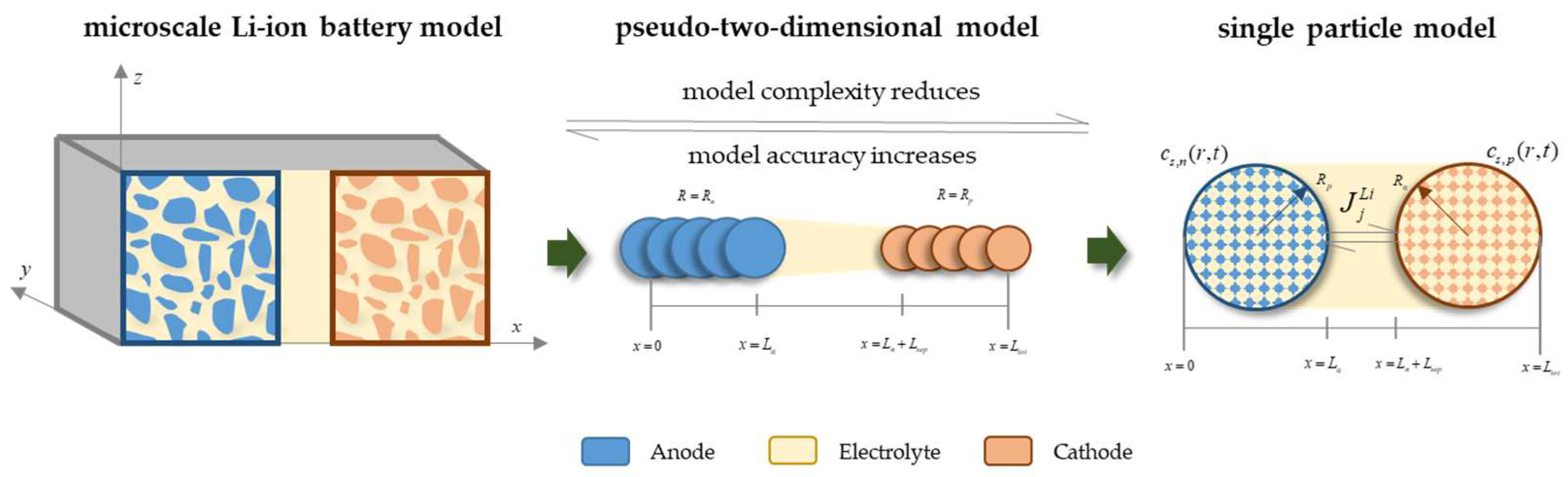
7]. On the contrary, the LIB mechanism model represented by the pseudo-two-dimensional (P2D) model [8] is very detailed in describing the dynamic of lithium-ion intercalation and deintercalation in microscale. In terms of mechanism, it explains the occurrences of concentration polarization and ohmic polarization within the LIB. However, the mechanism model of LIBs often require dozens of electrochemical parameters to be described and are composed of nonlinear partial differential equations (PDEs), which hinder its application in the on-board BMS [9]. Currently, the P2D model is mainly solved using numerical methods, such as the finite volume method (FVM) [10] or finite element method (FEM). There are also more complex but computationally efficient methods, like the explicit–implicit Runge–Kutta–Chebyshev method [11], as well as a numerical method that iteratively solves each subequation in a specific order [12]. These studies have used many techniques to improve the computational efficiency of the P2D model. However, due to the limitations of numerical methods, these approaches still demand a considerable amount of computing resources and time. Consequently, these approaches can only be considered in situations where computational resources are relatively sufficient and time requirements are not strict [13].
The single-particle model (SPM) [14], as a reduced-order version of the P2D model, simplifies the PDEs in the P2D model into a single PDE by assuming uniform current density in the electrolyte. This assumption dramatically improves the calculation speed of the model, making it applicable to on-board BMS. However, precisely because of the uniform current density assumption, the SPM ignores the concentration polarization of lithium ions in the direction between the positive and negative collector under the condition of a high C-rate. Due to the limited diffusion coefficient of the electrolyte, lithium ions cannot move smoothly, resulting in a significant deviation from the P2D model. To address this issue, many scholars have used methods to approximate the electrolyte lithium-ion concentration and potential inside the battery to eliminate the error of the SPM under high C-rate conditions [15,16,17]. Metha et al. [17] constructed a model with the parabolic equation and time-varying parameters, subject to boundary conditions and continuity conditions at interfaces of the P2D model. It approximates the lithium-ion concentration distribution in the cathode, anode, and separator. By solving a total of nine differential equations, the time-varying parameters for parabolic equations can be obtained. This method can effectively improve the accuracy of the SPM under high C-rate charge and discharge conditions. Assuming a parabolic curve for the distribution in lithium-ion concentration can result in inaccurate modeling, leading to system errors.
To speed the calculation process for PDEs in mechanism models, many scholars have attempted this in multiple directions, among which the recent research directions include a physics-based equivalent circuit [18,19] and order-reduction methods [20]. Li Y et al. [19] started from the P2D model, used FVM to divide the battery into multiple elementary sections (ESs), and established equivalent circuit models for equations in the P2D model. This method can achieve a solution with high-precision results. However, the establishment of this model is relatively complex. Gopalakrishnan et al. [20] utilized reduced-order models (ROMs) for LIBs and improved the efficiency of the singular value decomposition (SVD) step. However, the order reduction also resulted in the model’s loss of details and nonlinear behavior. The emergence of physics-informed neural networks (PINNs) [21,
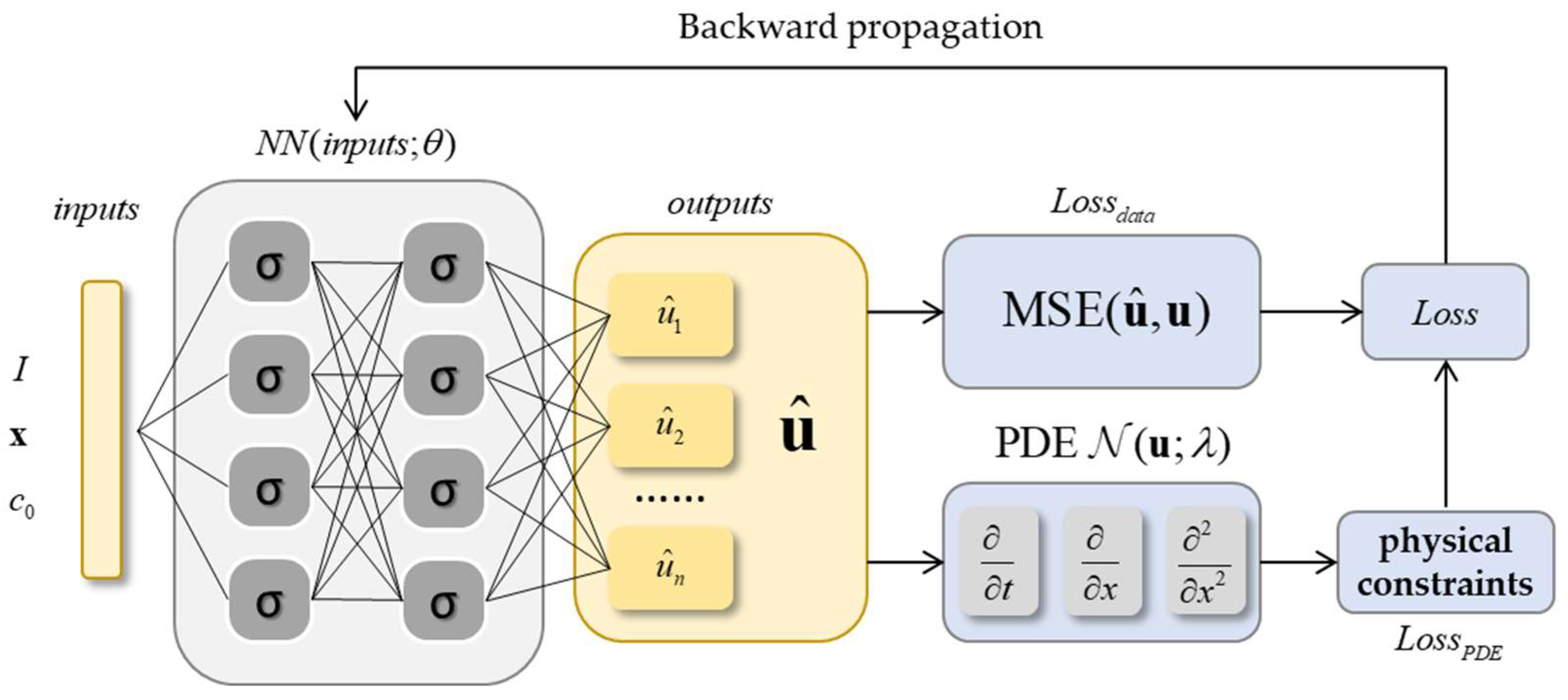
22] inspires the design of a LIB model that considers both calculation accuracy and efficiency. PINN was first proposed by Raissi et al. in 2018 [21]. This article explored using neural networks’ nonlinear function-fitting capabilities to solve physical problems described by PDEs. When managing PDEs, these equations often provide additional physical constraints that the neural network must consider. This is where PINN surpasses traditional neural networks, as it considers both data approximation and the information of PDEs when constructing the loss function. Training the neural network this way will lead to faster convergence and better generalization performance [22]. PINN has been successfully applied to many practical problems [23,24]. The excellent learning ability of PINN for the prior knowledge of physics provides a fast method for solving these complex PDEs. Misyris et al. [24] used PINN to predict the operation state of a power system, such as rotor angle and frequency. Chen et al. [23] designed WaveY-Net to calculate the electromagnetic field distribution in the structural medium to optimize and verify photonic devices. The network design is based on the classical encoder–decoder architecture and is realized by U-net based on a convolutional neural network. WaveY-Net only predicts the distribution of the magnetic field and uses Maxwell equation to calculate the electrical field, thus constraining the output of the neural network by physical information. WaveY-Net’s calculation speed is two to four orders faster than traditional methods.
There are also relevant studies using PINN [25,26,27,28] in the field of batteries. Li et al. [25] used 2d-LSTM to build a state observer for the key parameters for the P2D model. The network input is the voltage, applied current, temperature, and other sequence data during battery operation. The outputs are five key parameters for the battery model, one being the lithium-ion concentration. The highlight of this research is that it uses the simulation data from the P2D model calculated by FVM as the data set, which provides an idea for the application of PINN in the field of batteries. Pang et al. [26] used the PINN and constructed the bidirectional LSTM (BiLSTM) network model based on the Bayesian optimization algorithm (BOA) to predict the heat production rate (HGR) of the battery under specific applied current, a method that achieved good results. However, these mentioned researchers just drew lessons from the PINN because they did not use the additional physical constraints brought by the electrochemical model in constructing the loss function of neural networks. The training of neural networks in these studies relies more on the fitting of simulated data, which limits the ability of these networks to learn the mechanism of LIBs. Ref. [28] utilized physics-informed neural networks as a solver for the PDE of lithium-ion concentration diffusion in electrode particles. The established battery model was then used to estimate the battery’s state-of-charge (SOC) and state-of-health (SOH). In training the PINN network, the fully connected network (FCN) is used as the architecture of the PINN to approximate the particle concentration distribution of electrode particles under certain applied currents. Compared with other articles that describe constructing the loss function [25,26], it considers the physical constraints of differential equations and their boundary conditions. The network has a simple structure and only takes in particle radial coordinates R and time T as inputs. As a result, it can only learn about the lithium-ion diffusion process under specific applied current and electrochemical parameters, which severely restricts the application of the LIB model; when the applied current of the battery changes, the network needs to be retrained. Networks described in Ref. [29] can take any current sequence as input and output the terminal voltage of the cell. However, this method treats the battery as a black box and does not consider the mechanism of the battery. Therefore, it can only be an aging-independent model.
In contrast, our approach builds a LIB model using a recurrent neural network (RNN) as the architecture of the PINN and is based on the SPM. The network’s inputs are the coordinates x, initial lithium-ion concentration c 0 , and applied current I. This network, called SPM-Net, is used as a solver of the diffusion equation in the electrolyte. Compared with the network described in Refs. [28,29], this network can solve the distribution of electrolyte lithium-ion concentration under various applied current conditions, which has stronger adaptability and is extensible. The main contributions of this paper are as follows:
(1)
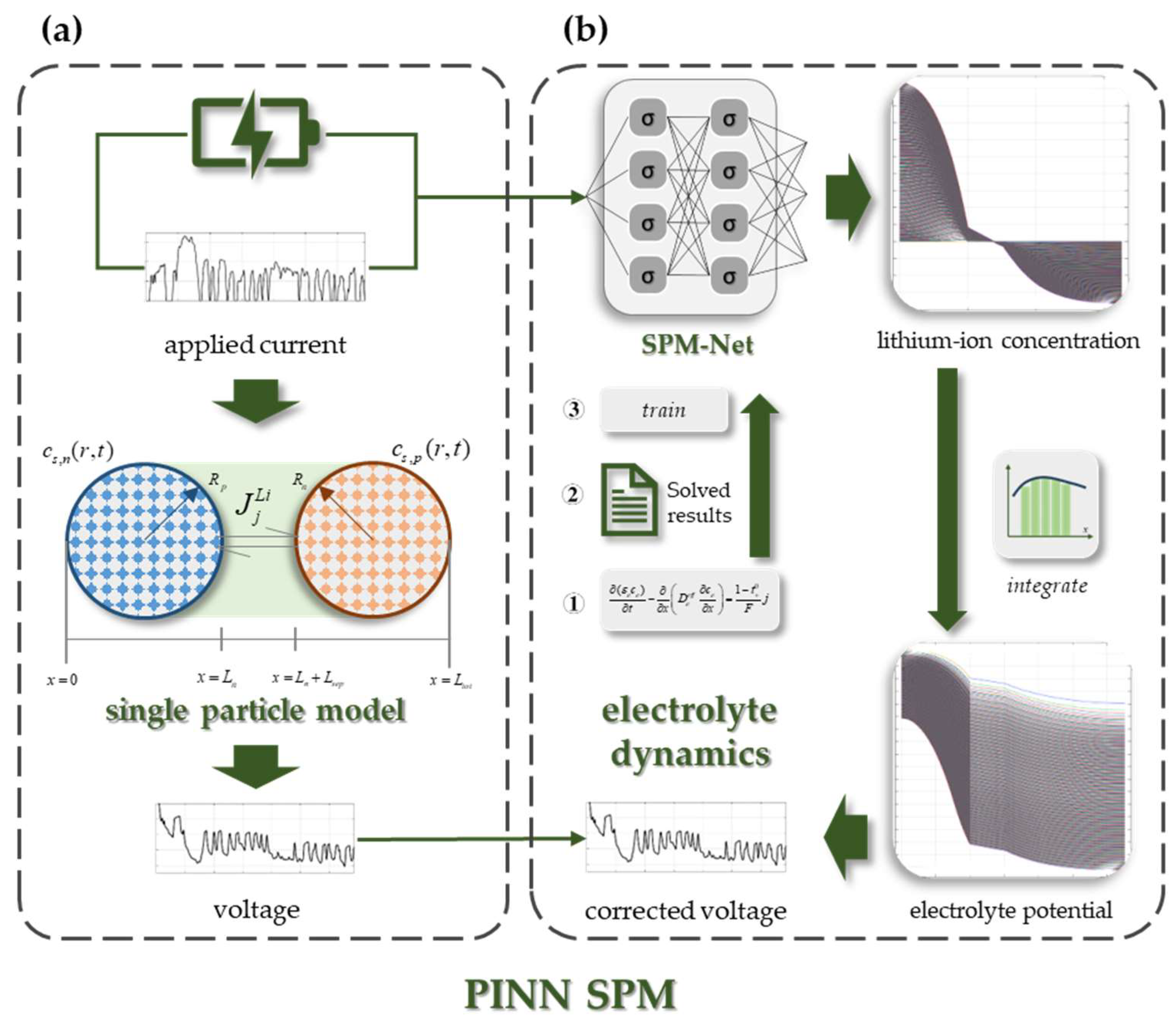
Establishment of an SPM with electrolyte dynamics called PINN SPM. This model greatly improves the accuracy of the SPM under high C-rates. It uses a PINN to approximate the lithium-ion distribution in electrolytes and then calculates the electrolyte potential distribution so that the error of the SPM can be eliminated.
(2)
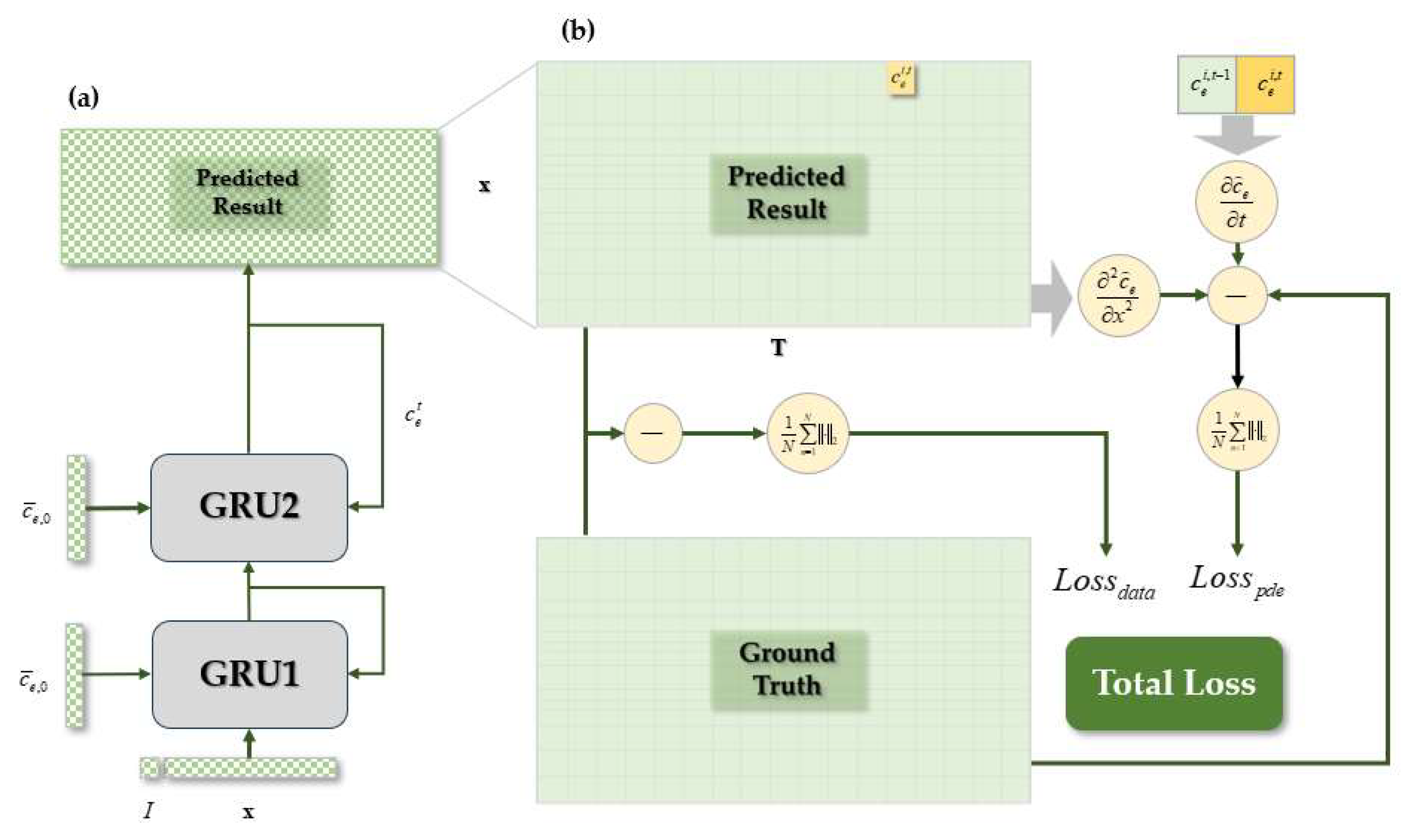
Creation of a physics-informed neural network called SPM-Net, which is the central part of PINN SPM. It can quickly solve the one-dimensional diffusion equation of the LIB model, which means the network can approximate the electrolyte lithium-ion concentration distribution under various applied currents with specific battery parameters.
(3)
Better performance of the battery electrochemical model. Using the physical constraints from PDE to design the loss function, SPM-Net can approximate the concentration results more accurately than the traditional neural network under dynamic conditions. Additionally, it is 20.8% faster than the traditional numerical method under dynamic conditions.
The remainder of this paper is organized as follows. Section 2 introduces the PINN SPM proposed in this paper. Section 3 introduces the structure of SPM-Net, data preparation, loss-function design approach, and training details of SPM-Net. The following part, Section 4, analyzes the accuracy and calculation efficiency of the PINN SPM compared with other methods. The conclusion of this paper is provided in Section 5.

2. Modeling of the LIBs

2.1. P2D Model

It is challenging to create an accurate 3D model of the electrode and electrolyte in batteries practically when using the microscale model. This is due to the electrode material’s porous nature and irregular shape, as shown in Figure 1. Therefore, it is necessary to simplify the microscale model further. For most LIBs, there is only polarization in the direction between the cathode and anode that significantly affects the battery terminal voltage. Hence, the microscale model can be simplified into one dimension. By averaging microscopic quantities over a finite but small unit of volume, a continuum-scale model can be established [30]. As shown in Figure 1, each point along the X dimension of the battery represents the average values in a small volume of the microscale model, where there are both electrode and electrolyte phases. Therefore, it is necessary to use the volume fraction of each phase to correct the material parameters at this point, such as the diffusion coefficient and the conductivity. The formula for the effective coefficient is given by:
θ x = s , e e f f = θ x = s , e ε x = s , e b r u g
where θ x = s , e represents any material parameter for the electrode phase or electrolyte phase, ε x = s , e is the volume fraction of this phase, and b r u g is called Bruggman’s exponent. According to experience and experimental data [31], b r u g is generally taken as 3.3.
To describe the diffusion process of lithium ions in the solid phase, the continuum model assumes that there is a spherical electrode particle to approximate the lithium-ion concentration diffusion in the electrode at each X coordinate. The model assumes a concentration gradient only in the radial direction. Therefore, the final model has two dimensions: X in the direction of cell thickness and R, specifically used to describe the radial gradient. Because dimension R is only related to c s , this is why the continuum model is also called the pseudo-two-dimensional model. P2D is the most widely used mechanism model for LIBs. It was first proposed by Doyle et al. [8] based on the concentrated solution theory and Fick’s diffusion law. It describes the dynamics of lithium-ion concentration and potential in the electrode particles and electrolytes through the conservation of mass and charge at microscale. Then, the Butler–Volmer equation couples the lithium-ion concentration distribution, potential distribution, and flux density on the particle surface. PDEs and boundary conditions for the P2D model are listed in Table 1.

2.2. Single-Particle Model

PDEs of the P2D model describe the mass conservation of lithium ions in the electrolyte and electrode of LIBs and the charge conservation in both electrolyte and electrode based on Ohm’s law, which makes it describe the polarization of the LIB during operation. However, because five PDEs couple it, solving these equations requires extensive computational resources. When the applied current is low, the internal polarization of the LIB is not apparent. It can be assumed that the electrolyte conductance is infinite, and the exchange current density is uniform in the X direction, so simply two spherical electrode particles can represent the LIB’s cathode and anode, respectively. This reduced-order model is called SPM, in which the terminal voltage can be expressed as [32]:
V ( t ) = Φ s , p ( t ) Φ s , n ( t )   = η p + U p ( C s e , p ) + ϕ e , p η n U n ( C s e , n ) ϕ e , n
where U i , i = n , p represents the open circuit voltage (OCV) of the positive and negative electrode materials varying with the lithium-ion concentration on the electrode surface, and η i , i = n , p is the overpotential of the positive and negative electrodes. It is related to the flux across the solid–electrolyte interface j i , i = n , p . The relationship between overpotential and flux density is described by the Butler–Volmer equation, which is given by:
j i = j 0 , i [ exp ( α a F η i R T ) exp ( ( 1 α a ) F η i R T ) ]
where j 0 , i = k i ( C max , i C s e , i ) α a C s e , i 1 α a C e , 0 α a .
Under the assumption of uniform current density, the molar flux density can be directly calculated from the battery applied current I , and the formula is:
j i = ± I a s , i F L i
Ignoring the influence of the voltage drop on the electrolyte and the change in lithium-ion concentration in the electrolyte, the final formula for calculating the battery terminal voltage of the SPM can be expressed as:
V ( t ) = Φ s , p ( t ) Φ s , n ( t )   = ( U p ( c s e ) U n ( c s e ) )         + R T α a F sinh 1 [ I 2 a s , p F L p j 0 , p ( C s e , p ) ] R T α a F sinh 1 [ I 2 a s , n F L n j 0 , n ( C s e , n ) ]

2.3. Establishment of PINN SPM

2.3.1. SPM with Electrolyte Dynamics

Two assumptions were made while establishing the SPM: lithium-ion concentration remains constant during battery operation, and the electrolyte potential is negligible. These two assumptions lead to large errors between the SPM and P2D model simulation results under high C-rates. To improve the accuracy of traditional single-particle models, a considerable number of studies have been made to establish the SPM with electrolyte dynamics [17,33,34]. Among these, Ref. [17] uses quadratic polynomials to model the lithium-ion concentration distribution of electrolytes in the cathode, anode, and separator:
C ¯ e , i = a i , 0 ( t ) + a i , 1 ( t ) x i + a i , 2 ( t ) x i 2
With the constraints of the boundary conditions and continuity conditions at interfaces introduced in Formulas (2)–(6), the time-varying parameters a i , k can finally be solved from total nine differential equations, where i = n , s , p , k = 0 , 1 , 2 .
The average value of electrolyte lithium-ion concentration inside the positive and negative electrodes is used to correct the effect on j 0 , i , and the time-varying parameters a i , k are used to correct the effect of ignoring the electrolyte potential. Therefore, the terminal voltage of the SPM with electrolyte dynamics can be expressed as [17]:
V ( t ) = ( U p ( c s e ) U n ( c s e ) )     + R T α a F sinh 1 [ I 2 a s , p F L p j 0 , p ( C s e , p , C e , a v g ) ] R T α a F sinh 1 [ I 2 a s , n F L n j 0 , n ( C s e , n , C e , a v g ) ]     I [ L p 3 κ p e f f + L s κ s e f f + L n 3 κ n e f f + L p 3 σ p e f f + L n 3 σ n e f f ]     R T ( t + 0 1 ) F [ 2 ( a n , 1 + 2 a n , 2 ) 3 ( a n , 0 + a n , 1 + a n , 2 ) + ( a s , 1 + 2 a s , 2 ) ( a s , 0 + a s , 1 + a s , 2 ) + a s , 1 a s , 0 + 2 a p , 1 3 a p , 0 ]
where κ i e f f is the effective conductivity of electrolyte.
The SPM with electrolyte dynamics modifies the traditional SPM by considering electrolyte concentration and potential distribution. This method uses quadratic polynomials with time-varying parameters to fit the distribution of electrolyte lithium-ion concentration and electrolyte potential. However, systematic errors exist in modeling the electrolyte lithium-ion concentration distribution through a parabola. The lithium-ion concentration distribution has some error compared with that simulated by the P2D model. Aiming to establish a more accurate and efficient SPM, the kernel part of the model called PINN SPM proposed in this paper is as follows.
(1)
In the PINN SPM, it is assumed that the exchange current density is uniform inside the battery, so the electrolyte lithium-ion concentration distribution can be obtained by only solving the diffusion equation in Formula (2).
(2)
Based on the previous step, the distribution of lithium-ion concentration in the electrolyte is solved by Formula (2) under different applied currents. These solved results are divided into data set, validation set, and test set, which are utilized for SPM-Net training.
(3)
SPM-Net is a PDE solver and replaces numerical methods for solving the diffusion equation to accelerate the solving speed.
The specific process of the PINN SPM can be seen in Figure 2. Figure 2a shows the process of the SPM and Figure 2b illustrates how to consider electrolyte dynamics to correct the SPM result. In Figure 2b, SPM-Net, which is trained from solved results, takes current as input and approximates the lithium-ion concentration. The concentration affects the conductivity of electrolyte, and then the electrolyte potential can be integrated according to the conductivity. Finally, with the rectification from electrolyte potential, results from the SPM are more accurate. Theoretically, the neural network can fit any function. Therefore, compared with the time-varying parabolic equation, it can greatly improve the accuracy for the approximation of lithium-ion concentration in LIBs so that the accuracy of the LIB model is also improved.

2.3.2. Physics-Informed Neural Networks

As an effective method for solving PDEs, PINNs have the characteristics of high accuracy and high efficiency. PINNs were first proposed in 2018 [21,22]. Compared with the traditional neural network, which fits the data, the physics-informed information from PDEs is also considered in the training process for the PINN. As shown in Figure 3, using a neural network framework like Pytorch, the derivative of the neural network output with respect to the input can be obtained, which can be substituted in the PDEs to construct the loss function. The neural network trained through this method is more generalized.
SRM-Net proposed in this paper is the solver for the diffusion equation in the electrolyte. It establishes the relationship between applied current and lithium-ion concentration of the electrolyte. Specifically, the input of SPM-Net is the applied current at time t ; the mesh x , where the concentration is to be calculated; and the initial lithium-ion concentration distribution c 0 . The output of the network is the lithium-ion concentration vector on mesh x at time t + 1 . The network is used to manage sequence problems, that is to say, the output of the lithium-ion concentration of the network at the current time t is used as the input for the initial lithium-ion concentration distribution c 0 at the next time t + 1 . To achieve this, SPM-Net uses the gated recurrent unit (GRU) as the network architecture.
The GRU was proposed by Cho et al. [35] in 2014. Compared with the traditional RNN, it can be trained to retain information from further back. Additionally, its network architecture is more concise, which means that GRU uses fewer training parameters and therefore uses less memory and executes faster than long short-term memory (LSTM) [36], while its performance is not inferior to that of LSTM. In Section 4, the learning abilities of different recurrent network units for the diffusion equation solver are specifically discussed. Similar to LSTM, GRU calculates internal states H t at each time step based on the output H t 1 of the previous time and the input X t of the present time. The calculation of internal state H t is achieved through the use of two gates, including the update gate Z t and reset gate R t . The calculation formula is given by:
R t = σ ( X t W x r + H t 1 W h r + b r ) Z t = σ ( X t W x z + H t 1 W h z + b z ) H ˜ t = tanh ( X t W x h + ( R t H t 1 ) W h h + b h ) H t = Z t H t 1 + ( 1 Z t ) H ˜ t
where W , b are network parameters and H ˜ t is the candidate hidden state. The specific architecture of GRU is shown in Figure 4.
In SPM-Net, the input vector X t is the applied current I at time t concatenated with the mesh x , and the initial value of the hidden state is the initial lithium-ion concentration distribution c 0 on the mesh. The output vector of SPM-Net is the lithium-ion concentration c e at each time step. The step length of the time series is 1 s. In this way, the network can act as a diffusion equation solver. See Section 3 for the specific structure and training methods for SPM-Net.
According to the electrolyte charge conservation, Equation (4), assuming that the exchange current is uniformly distributed, the electrolyte potential distribution can be calculated by a numerical method:
ϕ e , i x = 2 R T ( 1 t + 0 ) F ln c e x a s , i F κ e f f j i d x
ϕ e ( L t o t ) ϕ e ( 0 ) = 2 R T ( 1 t + 0 ) F ( ln ( c e ( L t o t ) ) ln ( c e ( 0 ) ) ) a s , i F κ e f f 0 L t o t j i d x
So far, the PINN SPM can be expressed as:
V ( t ) = ( U p ( c s e ) U n ( c s e ) )     + R T α a F sinh 1 [ I 2 a s , p F L p j 0 , p ( c s e , p , c e , a v g ) ] R T α a F sinh 1 [ I 2 a s , n F L n j 0 , n ( c s e , n , c e , a v g ) ]     + ϕ e ( L t o t ) ϕ e ( 0 )

3. Method

3.1. Data Preparation

The data set for SPM-Net proposed in this paper is simulated by MATLAB and the P2D model results are simulated through the software COMSOL Multiphysics 5.6. The electrochemical parameters for the LIB are shown in Table 2 [31,37]. The cell chemistry comprises LixC6 as the negative electrode, LiyMn2O4 as the positive electrode, and LiPF6 in 2:1 EC: DMC as the electrolyte. The 1C-current density of the cell is 17.5 A / m 2 . The open circuit voltage (OCV) of the positive and negative electrode materials is approximated by Formulas (24) and (25), where θ i , i = p , n is the ratio of the lithium-ion concentration on the particle surface to the maximum lithium-ion concentration of the electrode, which is the SOC of the electrode. The SPM [14] and the SPM with electrolyte dynamics in Ref. [17] are also solved and simulated by MATLAB. For the proposed model, it is also simulated using MATLAB, where the concentration distribution of electrolyte lithium ions is obtained by calling the Pytorch framework. All simulations are performed on a PC with a 6-core AMD Ryzen 5 5600H CPU and Radeon Graphics @ 3.3 GHz, with 16 GB (3200 MHz) of memory.
The lithium-ion concentration distributions of the positive and negative electrolyte of the battery under different current rates and dynamic conditions are simulated. The static current varies from −4.3 to −1C and 1 to 4.3C. When the battery terminal voltage reaches the battery cutoff voltage or the simulation time exceeds the maximum time, the simulation ends. In this simulation, the cutoff voltage of the battery is set to 4.2–3 V, and the maximum simulation time is 10,000 s. There are 47 nodes on mesh x , and the distance between them is not equal. The grid is denser near the discontinuous parts, where there are interfaces between cathode, anode, and separator. The training set and validation set of the network are the data simulated from charge and discharge conditions with static current, and the test set consists of the data obtained from the battery under the condition of dynamic applied current.

3.2. Network Architecture

To better learn the distribution of electrolyte lithium-ion concentration under different applied current conditions, the network uses double-layer GRU architecture, which has more training parameters and better learning ability. The specific network architecture is shown in Figure 5.
The input of the GRU network is the applied current at each time step concatenated with the mesh x , and the output c e is the corresponding electrolyte lithium-ion concentration on the grid at each time step. Using the autograd function in Pytorch, the second derivative of the SPM-Net output with respect to the input mesh x can be obtained as:
2 c e i , t x i 2 = 2 N N ( I , x i ) x i 2
The time derivative of lithium-ion concentration is replaced by the first-order backward difference equation, which is:
c e i , t t = c e i , t c e i , t 1 Δ t
where c e i , t represents the electrolyte lithium-ion concentration at the ith sampling point in the x direction of the battery model at time t.
The loss function is divided into two parts: one part is the root mean squared error (RMSE) between data and predicted results, called L o s s d a t a ; The other part is the value generated by substituting the derivative of the network output into the differential equations, called L o s s p d e . The total loss can be expressed as:
L o s s = ( 1 β ) L o s s d a t a + β L o s s p d e
L o s s d a t a = 1 N n = 1 N c e ( n ) c e ( n ) 2
L o s s p d e = 1 N n = 1 N ε e c e t D e , e f f 2 c e x 2 a s ( 1 t + 0 ) j i 2
where β is a hyperparameter in which 0.2 is used for optimal performance; its influence on the training of PINN is discussed in the next section. c e represents the data obtained by the MATLAB simulation, while c e , c e t , 2 c e x 2 in Formulas (17) and (18) is the derivative of the prediction result from the PINN with respect to the network input.

3.3. Training Method

To ensure the convergence of training, the original simulation data should be normalized after it is obtained. For the lithium-ion concentration of electrolyte, the initial concentration c 0 = 2000   mol / m 3 is set as the reference lithium-ion concentration c r e f , and the normalized lithium-ion concentration data c ¯ e is:
c ¯ e = c e / c r e f 1
The input x i , i = n , p with respect to its electrode length L i , i = p , n is normalized:
x n = x / L n , x p = ( x L n L s ) / L p
The learning rate for training is set to 1 × 10⁻³, and when the 300th and 600th epochs are trained, the learning rate becomes 30% of that before. This learning rate schedule is determined after multiple attempts to ensure smooth and fast convergence of the network. Using Adam as the optimizer, the final training results are analyzed and discussed in Section 4. All training is conducted on a workstation with a 12-core Intel (R) Xeon (R) Platinum 8255C CPU @ 2.50 GHz.
U n = 0.16 + 1.32 exp ( 3 θ n ) + 10 exp ( 2000 θ n )
U p = 4.19829 + 0.0565661 tanh ( 14.5546 θ p + 8.60942 ) 0.0275479 [ 1 ( 1 y p ) 0.492465 1.90111 ] 0.157123 exp ( 0.04738 θ p 8 ) + 0.810239 exp [ 10 ( θ p 0.133875 ) ]

4. Simulation Results

4.1. Verification of the Solving Methods for Diffusion Equation in the Electrolyte

To obtain more accurate results for the battery terminal voltage, the accuracy of the lithium-ion concentration distribution should be ensured. This part demonstrates the most accurate method for obtaining lithium-ion concentration distribution. We compare solving the diffusion equation with fitting the parabolic equation [17].
Figure 6 compares the calculation results from the method proposed in this paper, the simulation results from the P2D model, and the results of the parabola method proposed in Ref. [17] under a 3C discharge condition. In the following part of this article, the method in Ref. [17] is called SPM2, which is calculated by solving a total of nine differential equations and substituting the results in Formulas (14) and (15). The method, which solves the diffusion equation numerically to obtain the concentration, is called the diffusion equation method (DEM), and the SPM uses electrolyte dynamics from the DEM is called the DEM SPM. There is an error between the DEM, SPM2, and P2D model results. Due to the assumption of uniform current density, the error is concentrated at both ends of the battery near the collector. It can be clearly observed from Figure 6c,e that compared with SPM2, the error of electrolyte lithium-ion concentration calculated by the DEM is lower.
Moreover, the electrolyte potential distribution ϕ e can be calculated by substituting the calculated lithium-ion concentration distribution into Formula (15). By observing Figure 7, it can be found that under high C-rate, the electrolyte potential distribution obtained by the DEM is closer to the results of the P2D model. Therefore, solving the diffusion equation can provide more accurate terminal voltage results, which qualifies the PINN SPM as having a more solid theoretical basis.

4.2. Comparison of Various Neural Networks

For a faster solver of the diffusion equation, the PINN SPM uses SPM-Net instead of the DEM to solve the diffusion equation. In this part, we discuss why GRU is to be used as the architecture for SPM-Net and why the PINN is used as the solver for the one-dimensional diffusion equation.
The PINN is constructed based on neural network architecture with a strong learning ability for accurate data fitting. Therefore, this part analyzes the learning ability of different architectures of recurrent neural networks for the one-dimensional diffusion equation. RNN, GRU and LSTM cells are used to learn the generated data, and the learning rate and optimizer are set according to the description provided in Section 3. Figure 8 records the changes in the RMSE for the training set and validation set in different epochs. It can be found that the RNN cell has the worst learning ability on this problem because of its simple architecture. LSTM and GRU cells perform well on the training set and can achieve high accuracy. Among them, GRU cells can achieve deeper overfitting for this problem. At the same time, the GRU training is faster with fewer parameters. Therefore, the GRU cell is chosen as the basis architecture for SPM-Net. In addition, it can also be found that when the number of epochs reaches more than 600, the loss of the validation set barely decreases, while the loss of the training set decreases slightly. Too many training times lead to overfitting of the neural network, so the number of iterations for the final training of SPM-Net is set to 650. The training-time comparison is shown in Table 3.
Discussion of the difference between training results from the traditional neural network and the PINN is in this section. While training the GRU, we tried to add physical constraints to the loss function (PINN) and not add (only-data). Table 4 shows these two neural networks’ final performance on the validation and test sets. The only-data neural network and the PINN can be effectively used as the diffusion equation solver, and the RMSE can be very low in the validation set, 6.63 × 10⁻⁵ of only-data and 6.72 × 10⁻⁵ of the PINN. However, it is insufficient to just ensure the excellent results of L o s s d a t a . To obtain better results in L o s s p d e is also vital, which is closely related to the performance of the neural network under dynamic conditions. Low L o s s p d e leads to a better understanding of the physical information from the changes in the applied current in the test set with dynamic conditions. From Table 4, it can be seen clearly that the PINN performs better than only-data on test set: 2.18 × 10⁻⁴ for only-data and 1.23 × 10⁻⁴ for the PINN. Additionally, the PINN also has lower L o s s p d e : 1.03 × 10⁻² for only-data and 2.02 × 10⁻⁴ for the PINN. These results demonstrate that the PINN has better generalization than the only-data network.
The impact of different values of hyperparameters β in Formula (19) on training the PINN is also discussed. If β is too small, the neural network cannot learn additional information from physical constraints. However, when β is too large, the neural network has difficulty capturing the information owned by the data itself, and thus cannot obtain a good training effect. Figure 9 shows the training results for the PINN under different values of hyperparameter β . It can be found that when β is 0.2, the training result is improved. Setting β to 0.2 in SPM-Net, then the final PINN SPM is constructed.

4.3. Model Assessment

This part describes the accuracy and efficiency of the PINN SPM in contrast to other SPMs with electrolyte dynamics. The terminal voltage of the cell can be obtained by substituting the lithium-ion concentration obtained by SPM-Net into Formulas (14)–(16). Figure 10 and Figure 11 show the comparison of the terminal voltage from the PINN SPM, P2D simulation results, SPM results, and SPM2 results under different applied currents. Figure 11 compares the PINN SPM with the SPM2 and the SPM to demonstrate its accuracy. The simulation currents of ±1C and ±3C are chosen as they are the most representative conditions for these battery models. The reason behind selecting these currents is that ±1C can represent the most commonly occurring operation condition in practice, and ±3C can represent the battery model under high C-rates. As can be seen in Figure 11, the maximum error in terminal voltage from the PINN SPM is no more than 1% under both high and low applied currents. At high C-rate, the error of the PINN SPM is significantly lower than that of the SPM and SPM2. It is worth noting that the error of the PINN SPM increases at the end of the simulation under 1C discharge. This is because the change in lithium-ion concentration in the electrolyte at low current is trivial, and the exchange current density conforms to the assumption of uniform current density. However, with the discharging, the exchange current density distribution changes and gradually does not conform to the uniform current distribution, so the error becomes larger than in the previous period.
This part also includes the discussion of the comparison between the PINN SPM, SPM, and SPM2 under dynamic discharge conditions. Figure 12a shows the plot of discharge current, and its maximum current does not exceed 70   A / m 2 , which is 4C. It can be found that under the dynamic discharge condition, the PINN SPM can still capture the electrolyte dynamics of the battery and obtain better effect than the SPM2. The maximum relative error is 1.2% when the applied current increases rapidly.
Table 5 shows the mean absolute error (MAE) between the SPMs and P2D models. SPMs with electrolyte dynamics are excellent models whether or not it is a static or dynamic condition. Due to a more precise approximation of lithium-ion concentration, the DEM SPM and PINN SPM have better accuracy under all conditions. Approximation of the PINN SPM is obtained from SPM-Net; errors may be present when compared to the result of DEM SPM. As a result, the accuracy of the PINN SPM may be slightly lower than DEM SPM.
Table 6 shows the comparison of the solving time for different battery models. The DEM SPM comprises one diffusion equation, the SPM2 comprises nine differential equations, while the P2D model comprises five PDEs. It can be found that the time to solve five PDEs is longer than that to solve a single PDE, and the time to solve a single PDE is higher than that to solve nine differential equations. Applying the PINN can significantly reduce the time consumption for solving the diffusion equation. Especially under dynamic current, the application of the PINN makes the calculation time for voltage 46 times faster than that for the P2D model, and 20.8% faster than that for the DEM SPM, which needs to solve partial differential equations. Although the calculation speed of the PINN SPM is slightly inferior to the SPM2, it has more accurate results than the SPM2, which is a compromise between accuracy and efficiency.

5. Discussions

5.1. Limitations and Future Directions

In this paper, a SPM with electrolyte dynamics is studied. It mainly utilizes the PINN to solve the electrolyte diffusion equation quickly and accurately to improve the accuracy of the SPM. It has made some progress in the combination of the PINN and LIB models, but at the same time, the method still has some limitations. First, the influence of the approximation of the solid phase diffusion equation on the model’s performance should have been considered. The main focus of this paper is on the efficiency and accuracy of different methods to obtain the lithium-ion concentration distribution in electrolytes instead of in the solid phase. This process has many calculation methods, and the results significantly affect the final SPM results. Second, the model established in this paper needs to consider battery degradation, which limits the application of this model in the on-board BMS. The battery will age with use, and the capacity and maximum power will decline. When aging occurs, the existing model may need to be retrained. The training process may be a problem when the battery is put into operation. The overall complexity can be even more complex than conventional physical model parameter identification schemes.
Because of the two shortcomings mentioned above, we plan to improve them in subsequent research. For the first point, we plan to use different methods to approximate the solid phase diffusion process in the next step. The methods will be compared, and they will be combined with the proposed method in this paper to obtain a more efficient and accurate model. For the second point, we plan to expand our existing model to include the aging factor of the battery. At present, there have been many studies on electrolyte-enhanced SPMs considering ageing, such as Refs. [33,38]. These studies can provide ideas for our follow-up research. When we incorporate aging factors into the model and ignore the influence of aging on the electrochemical parameters of electrolyte, SPM-Net does not need to be retrained. We will also conduct corresponding experiments in the follow-up research to study the effectiveness of this model with battery aging and hope to apply this model to battery SOC and SOH estimation.

5.2. Prospects for the Application of the PINN SPM

The modeling of LIBs is to estimate internal status better and evaluate the safety risks [39]. A growing body of literature has established approaches to these goals, including data-driven methods [40] and electrochemical methods [41]. Combined with these two methods, the PINN SPM presented in this paper is a new exploration in this field, which has the excellent characteristics of high accuracy and speed in dynamic and static conditions. With these characteristics, this hybrid model will be promising in estimating SOH and SOC. The PINN SPM can be used as the digital twin of LIB in BMS. As shown in Figure 13, because the calculation speed of the model is fast enough, the internal parameters for the battery can be obtained in a shorter time with a genetic algorithm. The internal parameters for the battery can be followed during the battery’s entire life, and they can be input as extracted features of the LIB into the data-driven model for SOC and SOH estimation.

6. Conclusions

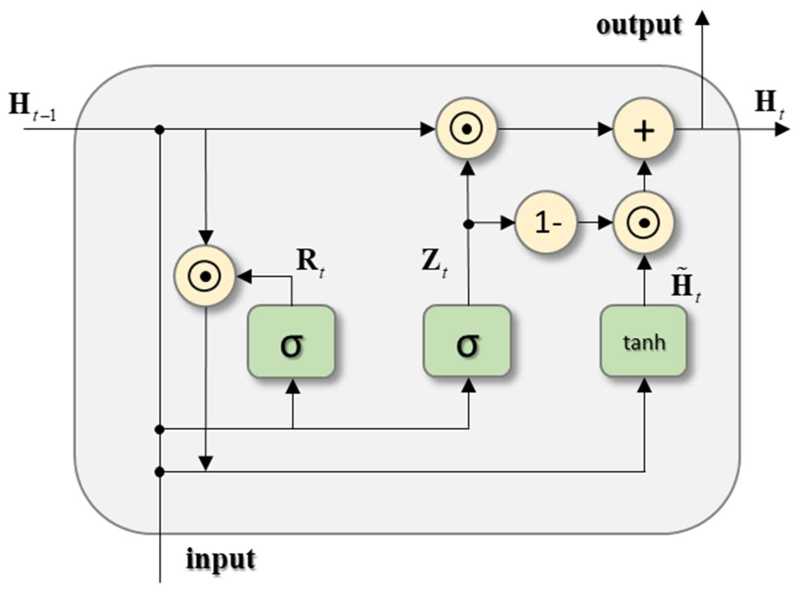
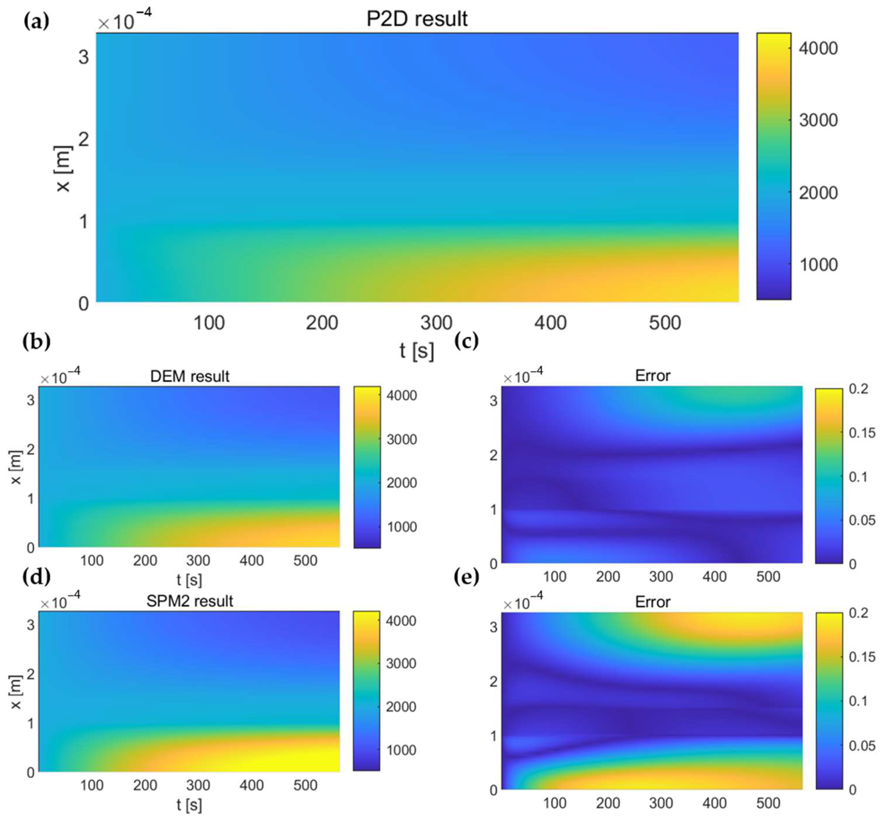
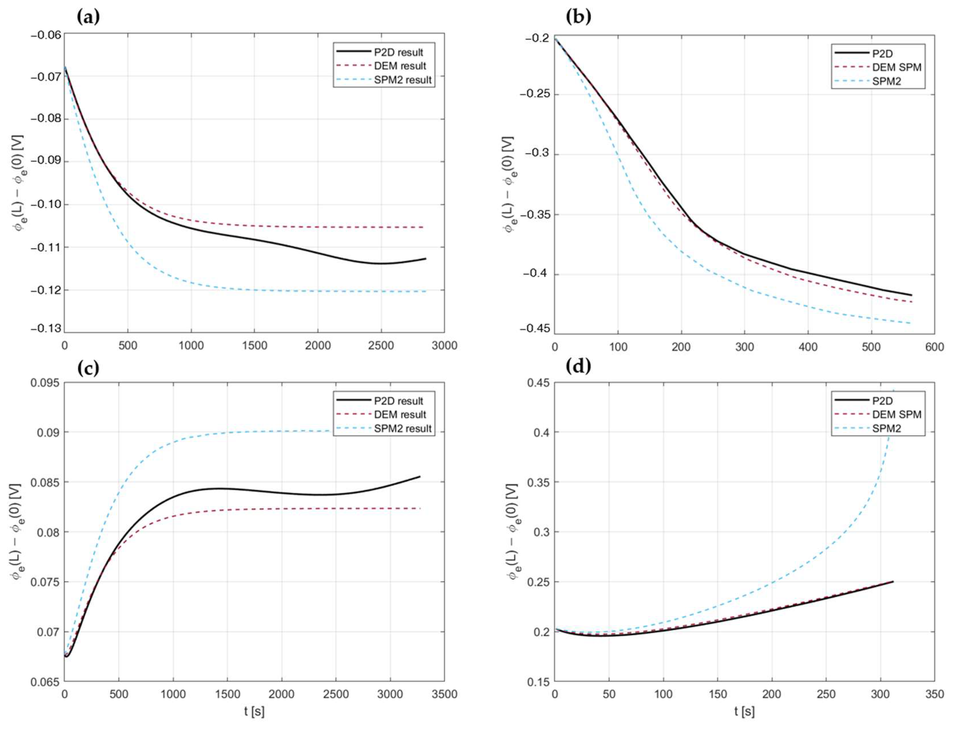
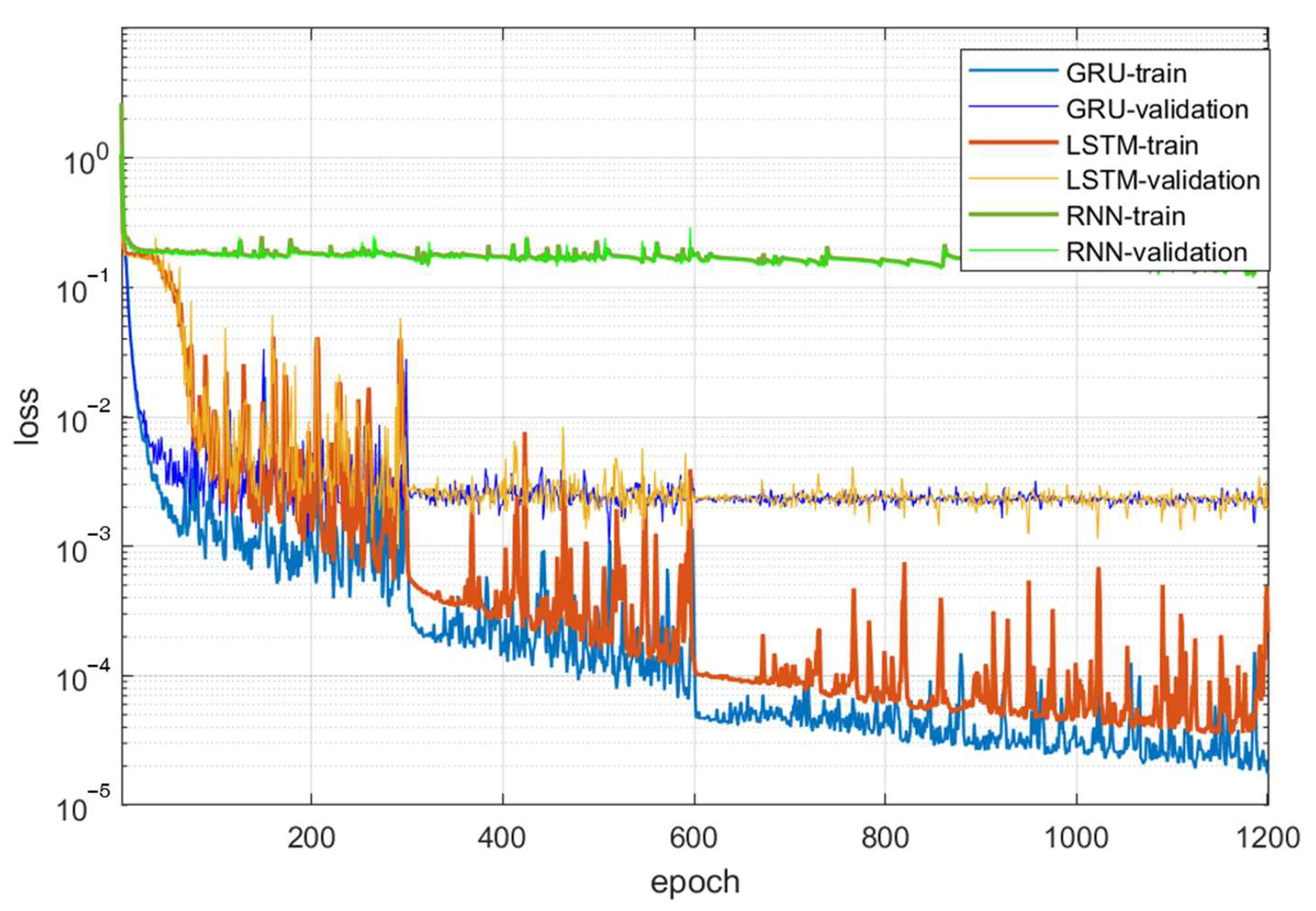
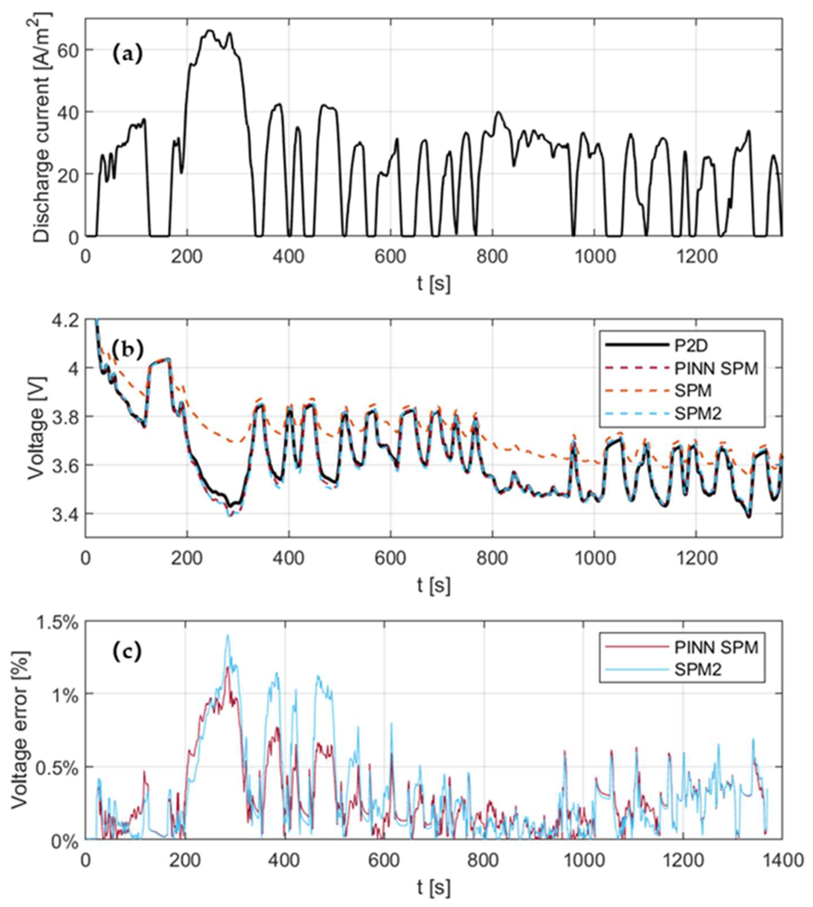
This paper proposes a more accurate SPM with electrolyte dynamics at high C-rates, called the PINN SPM, which has achieved good results compared with the traditional SPM with electrolyte dynamics. Firstly, a more accurate lithium-ion concentration distribution in the electrolyte can be obtained by solving the diffusion equation. Then, a GRU-based PINN called SPM-Net is designed to speed the solution of the diffusion equation. The PINN method exhibits better generalization performance compared to traditional neural networks under dynamic current conditions. Using SPM-Net as the solver for the diffusion equation, the calculation time of the battery model is 20.8% faster than that of the traditional method under dynamic conditions. Compared with the traditional SPM with electrolyte dynamics, the calculation accuracy of this model is higher, and the maximum relative error of the PINN SPM is less than 1.2% under dynamic and static charge conditions.
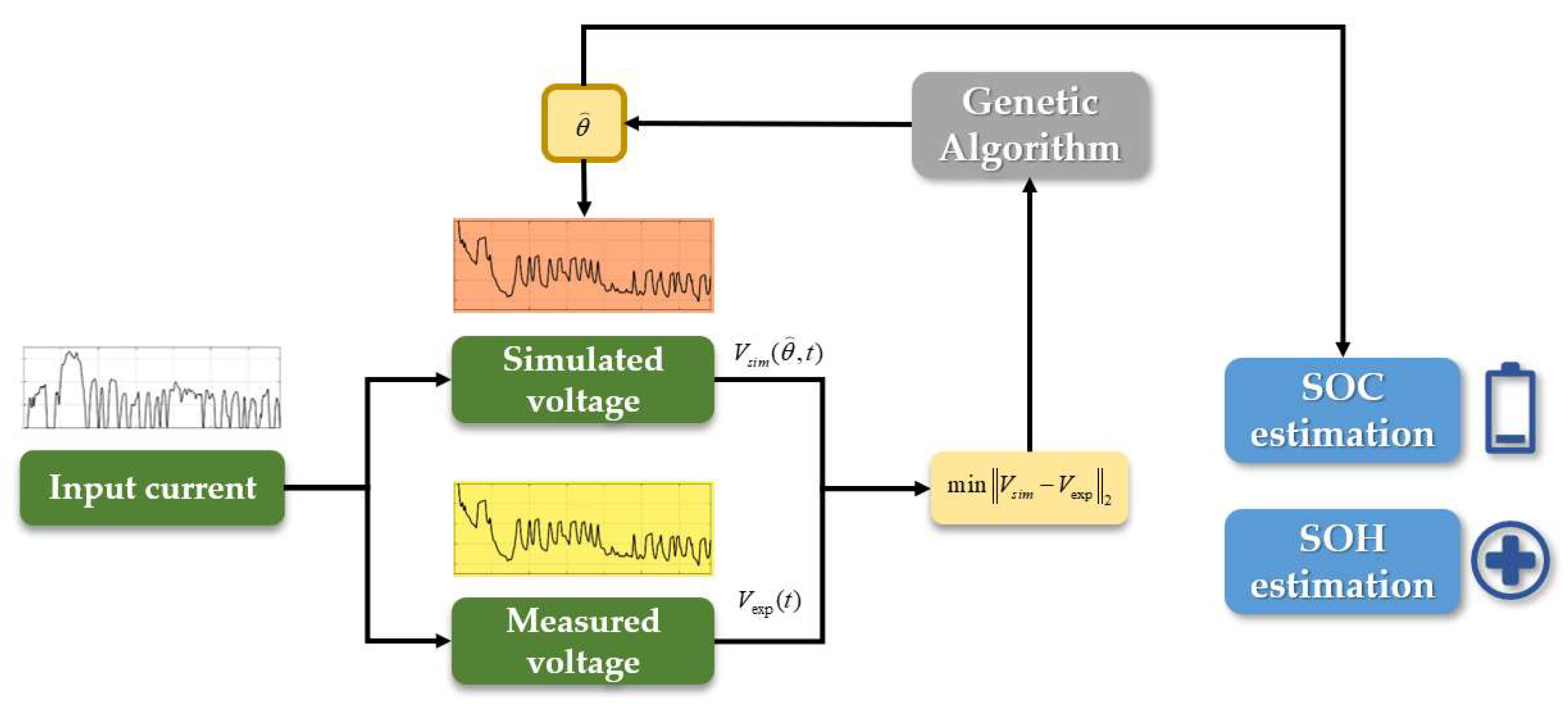
Nevertheless, the model proposed in this paper also has some drawbacks. For instance, the PINN SPM is higher in accuracy than the SPM2, but not in efficiency. Therefore, in future research, we plan to refine the SPM-Net architecture further to achieve improvements in both accuracy and efficiency. In addition, in the process for establishing the model, the PINN SPM only used simulated data and did not establish a connection between the model and the experiments. Therefore, establishing a PINN SPM based on the experimental data of the battery is also an important plan for future research. The purpose of all the modeling work for the LIB is to improve management. A genetic algorithm can be used to achieve parameter identification based on the model from experimental data. Then, by inputting these identified parameters as extracted features into the SOH and SOC estimation model, a hybrid method for BMS application can be finally achieved.

Author Contributions

Conceptualization, C.X., B.J. and H.D.; methodology, C.X. and B.J.; software, C.X., B.J. and J.Z.; validation, B.J. and X.W.; formal analysis, B.J. and X.W.; investigation, B.J. and H.D.; data curation, J.Z. and B.J.; writing—original draft preparation, C.X., B.J. and X.W.; writing—review and editing, J.Z. and H.D.; visualization, B.J. and X.W.; supervision, J.Z. and H.D.; project administration, H.D.; funding acquisition, B.J. and H.D. All authors have read and agreed to the published version of the manuscript.

Funding

This research was supported by the National Key R&D Program—Strategic Scientific and Technological Innovation Cooperation (Grant No. 2022YFE0207900), the National Natural Science Foundation of China (NSFC, Grant Nos. U20A20310 and 52307248), and the Shanghai Sailing Program (Grant No. 22YF1450400).

Data Availability Statement

Not applicable.

Conflicts of Interest

The authors declare no conflict of interest.

References

  1. Kim, T.; Song, W.; Son, D.Y.; Ono, L.K.; Qi, Y. Lithium-ion batteries: Outlook on present, future, and hybridized technologies. J. Mater. Chem. A 2019, 7, 2942–2964. [Google Scholar] [CrossRef]
  2. Chen, S.; Wei, X.; Zhang, G.; Wang, X.; Zhu, J.; Feng, X.; Dai, H.; Ouyang, M. All-temperature-area battery application mechanism, performance and strategies. Innovation 2023, 4, 100465. [Google Scholar] [CrossRef]
  3. Horiba, T. Lithium-ion battery systems. Proc. IEEE 2014, 102, 939–950. [Google Scholar] [CrossRef]
  4. Zhang, X.; Lu, J.; Yuan, S.; Yang, J.; Zhou, X. A novel method for identification of lithium-ion battery equivalent circuit model parameters considering electrochemical properties. J. Power Sources 2017, 345, 21–29. [Google Scholar] [CrossRef]
  5. Chen, W.; Liang, J.; Yang, Z.; Li, G. A review of lithium-ion battery for electric vehicle applications and beyond. Energy Procedia 2019, 158, 4363–4368. [Google Scholar] [CrossRef]
  6. He, H.; Xiong, R.; Guo, H.; Li, S. Comparison study on the battery models used for the energy management of batteries in electric vehicles. Energy Convers. Manag. 2012, 64, 113–121. [Google Scholar] [CrossRef]
  7. Jiang, B.; Zhu, Y.; Zhu, J.; Wei, X.; Dai, H. An adaptive capacity estimation approach for lithium-ion battery using 10-min relaxation voltage within high state of charge range. Energy 2023, 263, 125802. [Google Scholar] [CrossRef]
  8. Doyle, M.; Fuller, T.F.; Newman, J. Modeling of galvanostatic charge and discharge of the lithium/polymer/insertion cell. J. Electrochem. Soc. 1993, 140, 1526. [Google Scholar] [CrossRef]
  9. Wang, Y.; Kang, X.; Chen, Z. A survey of digital twin techniques in smart manufacturing and management of energy applications. Green Energy Intell. Transp. 2022, 1, 100014. [Google Scholar] [CrossRef]
  10. Torchio, M.; Magni, L.; Gopaluni, R.B.; Braatz, R.D.; Raimondo, D.M. Lionsimba: A matlab framework based on a finite volume model suitable for li-ion battery design, simulation, and control. J. Electrochem. Soc. 2016, 163, A1192. [Google Scholar] [CrossRef]
  11. Bermejo, R.; del Sastre, P.G. An implicit-explicit Runge-Kutta-Chebyshev finite element method for the nonlinear Lithium-ion battery equations. Appl. Math. Comput. 2019, 361, 398–420. [Google Scholar] [CrossRef]
  12. Han, S.; Tang, Y.; Rahimian, S.K. A numerically efficient method of solving the full-order pseudo-2-dimensional (P2D) Li-ion cell model. J. Power Sources 2021, 490, 229571. [Google Scholar] [CrossRef]
  13. Wang, X.; Li, J.; Chen, S.; Zhang, G.; Jiang, B.; Wei, X.; Dai, H. Online Detection of Lithium Plating Onset for Lithium-ion Batteries Based on Impedance Changing Trend Identification during Charging Processes. IEEE Trans. Transp. Electrif. 2022, 9, 3487–3497. [Google Scholar] [CrossRef]
  14. Ning, G.; Popov, B.N. Cycle life modeling of lithium-ion batteries. J. Electrochem. Soc. 2004, 151, A1584. [Google Scholar] [CrossRef]
  15. Li, J.; Lotfi, N.; Landers, R.G.; Park, J. A single particle model for lithium-ion batteries with electrolyte and stress-enhanced diffusion physics. J. Electrochem. Soc. 2017, 164, A874. [Google Scholar] [CrossRef]
  16. Liu, B.; Tang, X.; Gao, F. Joint estimation of battery state-of-charge and state-of-health based on a simplified pseudo-two-dimensional model. Electrochim. Acta 2020, 344, 136098. [Google Scholar] [CrossRef]
  17. Mehta, R.; Gupta, A. An improved single-particle model with electrolyte dynamics for high current applications of lithium-ion cells. Electrochim. Acta 2021, 389, 138623. [Google Scholar] [CrossRef]
  18. Von Srbik, M.T.; Marinescu, M.; Martinez-Botas, R.F.; Offer, G.J. A physically meaningful equivalent circuit network model of a lithium-ion battery accounting for local electrochemical and thermal behaviour, variable double layer capacitance and degradation. J. Power Sources 2016, 325, 171–184. [Google Scholar] [CrossRef]
  19. Li, Y.; Vilathgamuwa, M.; Farrell, T.; Tran, N.T.; Teague, J. A physics-based distributed-parameter equivalent circuit model for lithium-ion batteries. Electrochim. Acta 2019, 299, 451–469. [Google Scholar] [CrossRef]
  20. Gopalakrishnan, K.; Zhang, T.; Offer, G.J. A fast, memory-efficient discrete-time realization algorithm for reduced-order li-ion battery models. J. Electrochem. Energy Convers. Storage 2017, 14, 011001. [Google Scholar] [CrossRef]
  21. Raissi, M.; Perdikaris, P.; Karniadakis, G.E. Physics-informed neural networks: A deep learning framework for solving forward and inverse problems involving nonlinear partial differential equations. J. Comput. Phys. 2019, 378, 686–707. [Google Scholar] [CrossRef]
  22. Raissi, M.; Karniadakis, G.E. Hidden physics models: Machine learning of nonlinear partial differential equations. J. Comput. Phys. 2018, 357, 125–141. [Google Scholar] [CrossRef]
  23. Chen, M.; Lupoiu, R.; Mao, C.; Huang, D.H.; Jiang, J.; Lalanne, P.; Fan, J.A. High speed simulation and freeform optimization of nanophotonic devices with physics-augmented deep learning. ACS Photonics 2022, 9, 3110–3123. [Google Scholar]
  24. Misyris, G.S.; Venzke, A.; Chatzivasileiadis, S. Physics-informed neural networks for power systems. In Proceedings of the 2020 IEEE Power & Energy Society General Meeting (PESGM), Montreal, QC, Canada, 2–6 August 2020; pp. 1–5. [Google Scholar]
  25. Li, W.; Zhang, J.; Ringbeck, F.; Jöst, D.; Zhang, L.; Wei, Z.; Sauer, D.U. Physics-informed neural networks for electrode-level state estimation in lithium-ion batteries. J. Power Sources 2021, 506, 230034. [Google Scholar] [CrossRef]
  26. Pang, H.; Wu, L.; Liu, J.; Liu, X.; Liu, K. Physics-informed neural network approach for heat generation rate estimation of lithium-ion battery under various driving conditions. J. Energy Chem. 2023, 78, 1–12. [Google Scholar] [CrossRef]
  27. Nascimento, R.G.; Corbetta, M.; Kulkarni, C.S.; Viana, F.A. Hybrid physics-informed neural networks for lithium-ion battery modeling and prognosis. J. Power Sources 2021, 513, 230526. [Google Scholar] [CrossRef]
  28. Singh, S.; Ebongue, Y.E.; Rezaei, S.; Birke, K.P. Hybrid modeling of lithium-ion battery: Physics-informed neural network for battery state estimation. Batteries 2023, 9, 301. [Google Scholar] [CrossRef]
  29. Schmitt, J.; Horstkötter, I.; Bäker, B. Electrical lithium-ion battery models based on recurrent neural networks: A holistic approach. J. Energy Storage 2023, 58, 106461. [Google Scholar] [CrossRef]
  30. Plett, G.L. Battery Management Systems, Volume I: Battery Modeling; Artech House: London, UK, 2015. [Google Scholar]
  31. Doyle, M.; Newman, J.; Gozdz, A.S.; Schmutz, C.N.; Tarascon, J.M. Comparison of modeling predictions with experimental data from plastic lithium ion cells. J. Electrochem. Soc. 1996, 143, 1890. [Google Scholar] [CrossRef]
  32. Lotfi, N.; Li, J.; Landers, R.G.; Park, J. Li-ion battery state of health estimation based on an improved single particle model. In Proceedings of the 2017 American Control Conference (ACC), Seattle, WA, USA, 24–26 May 2017; pp. 86–91. [Google Scholar]
  33. Pang, H.; Mou, L.; Guo, L.; Zhang, F. Parameter identification and systematic validation of an enhanced single-particle model with aging degradation physics for Li-ion batteries. Electrochim. Acta 2019, 307, 474–487. [Google Scholar] [CrossRef]
  34. Rahimian, S.K.; Rayman, S.; White, R.E. Extension of physics-based single particle model for higher charge–discharge rates. J. Power Sources 2013, 224, 180–194. [Google Scholar] [CrossRef]
  35. Cho, K.; Van Merriënboer, B.; Gulcehre, C.; Bahdanau, D.; Bougares, F.; Schwenk, H.; Bengio, Y. Learning phrase representations using RNN encoder-decoder for statistical machine translation. arXiv 2014, arXiv:1406.1078. [Google Scholar]
  36. Hochreiter, S.; Schmidhuber, J. Long short-term memory. Neural Comput. 1997, 9, 1735–1780. [Google Scholar] [CrossRef] [PubMed]
  37. Park, J.; Seo, J.H.; Plett, G.; Lu, W.; Sastry, A.M. Numerical simulation of the effect of the dissolution of LiMn2O4 particles on Li-ion battery performance. Electrochem. Solid-State Lett. 2010, 14, A14. [Google Scholar] [CrossRef]
  38. Zhang, D.; Park, S.; Couto, L.D.; Viswanathan, V.; Moura, S.J. Beyond battery state of charge estimation: Observer for electrode-level state and cyclable lithium with electrolyte dynamics. IEEE Trans. Transp. Electrif. 2022, 7, 3199–3204. [Google Scholar] [CrossRef]
  39. You, H.; Zhu, J.; Wang, X.; Jiang, B.; Sun, H.; Liu, X.; Wei, X.; Han, G.; Ding, S.; Yu, H.; et al. Nonlinear health evaluation for lithium-ion battery within full-lifespan. J. Energy Chem. 2022, 72, 333–341. [Google Scholar] [CrossRef]
  40. Zhou, Z.; Liu, Y.; You, M.; Xiong, R.; Zhou, X. Two-stage aging trajectory prediction of LFP lithium-ion battery based on transfer learning with the cycle life prediction. Green Energy Intell. Transp. 2022, 1, 100008. [Google Scholar] [CrossRef]
  41. Qiao, D.; Wei, X.; Fan, W.; Jiang, B.; Lai, X.; Zheng, Y.; Tang, X.; Dai, H. Toward safe carbon–neutral transportation: Battery internal short circuit diagnosis based on cloud data for electric vehicles. Appl. Energy 2022, 317, 119168. [Google Scholar] [CrossRef]
Figure 1. Illustration of various LIB models at different scales, including microscale models, P2D models, and SPM, from left to right. From model 1 to model 2, the simulation difficulties caused by complex boundary shapes are simplified, while from model 2 to model 3 the computational complexity caused by coupling PDEs is simplified. However, simultaneously, the simplification sacrifices the model’s accuracy at high C-rates.
Batteries 09 00511 g001
Figure 2. Illustration of the PINN SPM process. (a) The SPM calculates the cell voltage through the applied current without considering the electrolyte dynamics. (b) Electrolyte dynamics corrects the voltage of the SPM by electrolyte potential obtained from the lithium-ion concentration. Moreover, the concentration is approximated from SPM-Net. It is a PINN and is trained by simulated data.
Batteries 09 00511 g002
Figure 3. Illustration of the basic concept and implementation approach of the PINN. It takes mesh x , loaded current I , and initial concentration c 0 as inputs, and outputs solutions to the PDE. Then, it uses the derivative of the result as a loss function to train the neural network.
Batteries 09 00511 g003
Figure 4. Basic architecture of GRU.
Batteries 09 00511 g004
Figure 5. Architecture of the diffusion equation solver SPM-Net and the design method of loss function. (a) The architecture of SPM-Net comprises two layers of GRU. Inputs of SPM-Net are two vectors. One is applied current concatenated with the mesh x , the other is the initial lithium-ion concentration c ¯ 0 . (b) The predicted result of SPM-Net is a tensor composed of lithium-ion concentration vectors at each time step. Two items are in total loss, L o s s d a t a and L o s s p d e . L o s s d a t a is obtained by calculating the root mean squared error (RMSE) between the predicted result and the ground truth, while L o s s p d e is obtained through differentiating the predicted result and substituting it into the PDE.
Batteries 09 00511 g005
Figure 6. Under 3C discharge current, the lithium-ion concentration distribution calculated by the DEM (b,c) and SPM2 method (d,e) and their relative errors. The electrolyte lithium-ion concentration distribution simulated by the P2D model is shown in (a).
Batteries 09 00511 g006
Figure 7. Simulation results for the electrolyte potential of the DEM and SPM2 methods and P2D model under 1C (a), 3C (b), −1C (c), and −3C (d).
Batteries 09 00511 g007
Figure 8. The loss of different recurrent neural network cell varies with epochs.
Batteries 09 00511 g008
Figure 9. Plot of the RMSE between the ground truth and the predicted lithium-ion concentration with respect to hyperparameter β .
Batteries 09 00511 g009
Figure 10. Comparison between the simulation results for different loading currents (±0.5C, ±1C, ±2C, ±3C, and ±4C) and the P2D model, where (a) is under the charge condition and (b) is the under the discharge condition.
Batteries 09 00511 g010
Figure 11. Comparison of terminal voltage results and relative errors between the proposed method, SPM2, and SPM methods under 3C (a,b), 1C (c,d), −3C (e,f), and −1C (g,h) conditions.
Batteries 09 00511 g011
Figure 12. Calculation results (b) and relative error (c) of the PINN SPM under dynamic conditions (a).
Batteries 09 00511 g012
Figure 13. Illustration of the future application of the PINN SPM.
Batteries 09 00511 g013
Table 1. Governing equations and boundary conditions for the P2D model [8].
Governing EquationsBoundary Conditions
Lithium-ion mass transport in electrolyte phase ( ε e c e ) t x ( D e e f f c e x ) = 1 t + 0 F j c e x | x = 0 , L t o t = 0 (2)
Lithium-ion mass transport in spherical particles c s t D s r 2 r ( r 2 c s r ) = 0 c s r | r = 0 = 0 c s r | r = R p = j i a s , i F (3)
Ohm’s law in electrolyte phase x ( κ e f f ϕ e x ) x ( κ D e f f ln c e x ) = j κ e f f ϕ e x + κ D e f f ln c e x | x = 0 , L t o t = 0 (4)
Ohm’s law in electrode phase x ( σ e f f ϕ s x ) = j ϕ s x | x = 0 , L t o t = ± I (5)
Butler–Volmer equation j = j 0 ( exp α a F R T ( η ) exp α c F R T ( η ) ) (6)
Table 2. Simulation parameters for the LIB cell [31,37].
ParameterAnodeCathode
Length   L [ m ] 100 × 10−6174 × 10−6
Particle   radius   R p [ m ] 8.5 × 10−612.5 × 10⁻⁶
Electrode   volume   fraction   ε s 0.4710.276
Electrolyte   volume   fraction   ε e 0.5290.724
Max .   solid   phase   concentration   C max [ m o l m 3 ] 26,39022,860
Stoichiometric at 100% state of charge0.5630.171
Stoichiometric at 0% state of charge0.0470.650
Diffusivity   in   the   electrode   D s [ m 2 s 1 ] 3.9 × 10−1410 × 10−14
Normalized   effective   reaction-rate   constant   k 0 , n o r m [ m 2.5 s 1 m o l 0.5 ] 2.2987 × 10−52.2042 × 10−5
Burg s   exponent   b r u g 3.3
Universal   gas   constant   R [ J ( m o l K ) 1 ] 8.3145
Temperature   T [ K ] 298.15
Faraday s   constant   F [ c m o l 1 ] 96875
Initial   electrolyte   concentration   c 0 [ m o l m 3 ] 2000
Diffusivity   in   the   electrolyte   D e [ m 2 s 1 ] 7.5 × 10⁻¹¹
Table 3. The training time of various recurrent neural networks per epoch.
GRULSTMRNN
time3 min 5 s3 min 35 s1 min 11 s
Table 4. Comparison of learning results with and without the PINN for the diffusion problems.
ValidationTest
Only-data L o s s d a t a 6.63 × 10−52.18 × 10−4
L o s s p d e 42.211.03 × 10−2
PINN L o s s d a t a 6.72 × 10−51.23 × 10−4
L o s s p d e 8.37 × 10−22.02 × 10−4
Table 5. Mean absolute error (MAE) in voltage for the DEM SPM, SPM2, PINN SPM under constant current discharge from 4.2 to 3 V and dynamic discharge condition.
Discharge RateDEM SPMSPM2PINN SPM
0.5C0.00200.00200.0020
1C0.00460.00500.0052
2C0.00990.01420.0118
3C0.01530.02160.0168
4C0.01410.03180.0207
Dynamic0.00940.01100.0099
Table 6. Time consumption comparison of various battery models under 1C, 2C, 3C, 4C, and dynamic discharge conditions.
Discharge RatePINN SPMDEM SPMSPM2P2D
1C0.53 s0.73 s0.68 s15 s
2C0.44 s0.52 s0.37 s8 s
3C0.24 s0.28 s0.22 s6 s
4C0.20 s0.29 s0.17 s5 s
Dynamic0.76 s0.96 s0.69 s36 s
Disclaimer/Publisher’s Note: The statements, opinions and data contained in all publications are solely those of the individual author(s) and contributor(s) and not of MDPI and/or the editor(s). MDPI and/or the editor(s) disclaim responsibility for any injury to people or property resulting from any ideas, methods, instructions or products referred to in the content.

