Article

Artificial Feature Extraction for Estimating State-of-Temperature in Lithium-Ion-Cells Using Various Long Short-Term Memory Architectures

Electrical Energy Storage Systems, Institute of Photovoltaics, University of Stuttgart, 70596 Stuttgart, Germany
*
Author to whom correspondence should be addressed.
Batteries 2022, 8(4), 36; https://doi.org/10.3390/batteries8040036
Submission received: 22 February 2022 / Revised: 9 April 2022 / Accepted: 11 April 2022 / Published: 15 April 2022
(This article belongs to the Special Issue The Precise Battery—towards Digital Twins for Advanced Batteries)

Abstract

:
The temperature in each cell of a battery system should be monitored to correctly track aging behavior and ensure safety requirements. To eliminate the need for additional hardware components, a software based prediction model is needed to track the temperature behavior. This study looks at machine learning algorithms that learn physical behavior of non-linear systems based on sample data. Here, it is shown how to improve the prediction accuracy using a new method called “artificial feature extraction” compared to classical time series approaches. We show its effectiveness on tracking the temperature behavior of a Li-ion cell with limited training data at one defined ambient temperature. A custom measuring system was created capable of tracking the cell temperature, by installing a temperature sensor into the cell wrap instead of attaching it to the cell housing. Additionally, a custom early stopping algorithm was developed to eliminate the need for further hyperparameters. This study manifests that artificially training sub models that extract features with high accuracy aids models in predicting more complex physical behavior. On average, the prediction accuracy has been improved by Δ T cell = 0.01   ° C for the training data and by Δ T cell = 0.007   ° C for the validation data compared to the base model. In the field of electrical energy storage systems, this could reduce costs, increase safety and improve knowledge about the aging progress in an individual cell to sort out for second life applications.

Graphical Abstract

1. Introduction

Motivation

Lithium-ion-battery technology is a promising energy storage technology for transitioning to electro-mobility due to its advantages, such as low self-discharge rate, long cycle life, scalability, high energy/power density, etc. To ensure safety requirements and longevity, cell parameters such as cell voltage U, cell current I and ideally cell temperature T cell need to be monitored at all times [1,2,3]. From these parameters, other vital cell states, such as state-of-charge SoC and state-of-health SoH, can be derived. The performance, longevity, safety, and applicability for second-life-applications are strongly dependent on the accuracy of these parameters. Obtaining the temperature T cell is especially challenging for two reasons. First, most battery systems work with temperature sensors that are attached to the cells’ housing. Thus, not the heat generation in the cell core is monitored, but the heat dissipation from the cell interior to the environment [3,4]. Furthermore, the cell temperature varies in a battery system depending on the location of the cell in a module [5,6]. Therefore, a sensor-based temperature tracking of each individual cell is recommended, however, not feasible in many applications. On the other hand, there are various software based prediction techniques such as mathematical–physical models and machine learning. However, physical models are highly computationally intensive [2,7], rely on information that is not available in real life applications [8,9,10] or is too specific to apply for every scenario that a battery is exposed to in real life applications. Some popular examples are finite element analysis, simulating the thermal field distribution by the Newman model [11], or the heat generation model by the Bernadi model [12]. In contrast, there are data-driven models, with their main advantages being transferability and universality [13]. Most data-driven models aim to make predictions about SoC [14] or SoH [15]. Temperature predictions using time series forecasts are rather rare and very specific. For example, Kleiner et al. [16] uses real life temperature data to make predictions for the future. The emphasis is thermal cause and thermal behavior over a cells lifetime in contrast to more complex real life situations that can have varying results [17,18,19].
This paper aims to compare artificial neural network (ANN) architectures to track thermal behavior of a single li-ion battery cell (LIBC) with a limited amount of training data and at a constant ambient temperature. This will show the impact of artificial feature extraction to improve the tracking capability of a physical non-linear systems.

2. Theoretical Foundations

This section will provide theoretical foundations regarding temperature behavior in LIBCs and the machine learning aspects used in this paper. First, it is shown how heat is generated and dissipated. This will give an insight of the complexity of dynamic non-linear systems such as LIBCs. Secondly, a short introduction to the machine learning aspects are given. The focus lays on recurrent neural networks to generate a time series forecast. It is important to notice, this section does not represent the scientific contributions gained by this paper, but shows the groundwork laid down by others.

2.1. Temperature Behavior in Lithium-Ion-Battery-Cells

The goal of this subsection is to gain an understanding of the complexity and investigate the necessary information to predict the temperature behavior in a LIBC. Therefore, we will look at the physical-thermal behavior of a single cylindrical LIBC. If we assume the internal temperature as well as the heat generation in a cell to be evenly distributed, we can derive from the law of energy conservation:
c cell m cell d T cell d t = Q gen + Q dis ,
with c cell representing the specific heat capacity, m cell the mass of the LIBC and d T cell d t the temperature change over time t [20]. Q gen is the heat generation rate and Q dis the heat dissipation rate. Equation (1) assumes that every additional heat source is infinitely far from the LIBC. In other words, the ambient temperature T amb is uniform.

2.1.1. Heat Generation

The heat generated inside a LIBC can be further subcategorized into reversible heat Q ˙ r , ohmic heat Q ˙ o , heat from material phase changes Q ˙ p and heat produced by the enthalpy absorbed or liberated from substances mixing Q ˙ m [3,20,21]. To simplify the model for heat generation, we will neglect voluminous expansion during charge and discharge cycles, assume that the active material is uniformly distributed and the diffusion coefficient of li-ion in solid particles is assumed as constant.
Reversible heat Q ˙ r is the energy needed to maintain the energy balance of the reaction caused by the gradient between the Gibbs free energy of product and reactant. Suppose the layer-by-layer cell structure is summarized as one block, the reversible heat Q ˙ r can be calculated by
Q ˙ r = I T cell U OCV T cell ,
with U OCV representing the open circuit voltage (OCV) potential [7,21,22]. U OCV is a function of the State-of-Charge (SoC) without the effects of overvoltage taken into account. Ohmic heat Q ˙ o is generated by collisions of charged particles in the solid and electrolyte phase and can be simplified by
Q ˙ o = I ( U U OCV ) ,
with (U- U OCV ) filtering the overvoltage [21]. Thus, for Q ˙ o , only the potential caused by the current load is analyzed. The heat from material phase changes Q ˙ p can be expressed by
Q ˙ p = i Δ H i a v g r i ,
and generally represents the heat either produced or consumed by the enthalpy change Δ H i a v g of a chemical reaction i multiplied by the rate r i at which the reaction i takes place [21,23,24]. Heat produced from mixing is calculated by
Q ˙ m = i ( H i ¯ H ¯ i a v g ) c i t d v ,
and is caused by the enthalpy H i ¯ absorbed or liberated by two or more substances mixing [24]. To isolate H i ¯ , the average concentration of the enthalpy H ¯ i a v g of i has to be subtracted and then multiplied by the concentration change over time c i / t . In a LIBC, this represents the formation and relaxation of concentration gradients within the LIBC and has to be integrated over it’s volume v. To obtain the total heat generated by a LIBC Q ˙ gen , all subcategories have to be summed up. However, it is worth knowing, that the impact of Q ˙ o and Q ˙ r far exceeds the impact of Q ˙ m and Q ˙ p .

2.1.2. Heat Dissipation

With the aim of gaining a full understanding of the thermal behavior of a LIBC, not only heat generation but also, heat dissipation Q dis needs to be taken into account. Q dis describes the heat escaping from the LIBC and is caused by three main phenomena: Radiation heat Q ˙ ra , convection heat Q ˙ cv and conduction heat Q ˙ cd .
Radiation heat Q ˙ ra describes the energy transport from its surface to the surrounding atmosphere and can be calculated by Stefan–Boltzmann law with
Q ˙ ra = ε σ A ( T out 4 T amb 4 ) ,
where ε represents emissivity (dependent on the materials and colors used), σ is the Stefan–Boltzmann constant, A is the surface area of the LIBC, T out is the surface temperature and T amb the ambient temperature [25]. Heat convection Q ˙ cv can be further subcategorized into forced and natural heat convection. In this study, we will only look at the natural Q ˙ cv . A simplified approximation is given by Jossen [26] with
Q ˙ cv = A c K , n ( T out T amb ) ,
with c K , n representing the constant of natural convection [25]. Heat conduction Q ˙ cd is caused by mechanical contact from the LIBC surface area A to other materials as well as the electrical wiring of the terminals. With Fourier’s law, we can derive
Q ˙ cd = k A d T out d x ,
as a one-dimensional representation x with the thermal conductivity between the two materials.
To summarize, aside from material constants and dimensional details, we would need information about the OCV, enthalpy behavior and concentration changes of several reactions and temperature data. In practical applications, this information is not accessible. This study aims to predict the temperature behavior with only the current profile I and its corresponding voltage response U without the need for solving differential equations.

2.2. Time Series Forecast

This section gives an overview of the machine learning aspects needed to follow along with this paper. ANNs are a subset of machine learning and at the heart of deep learning applications. A basic ANN is built with node layers, consisting of an input layer, a number of hidden layers, and an output layer [27]. Each layer has one or more neurons with individually associated weights and activation function. A training data set consists of labeled data points and is needed to train the weights [28]. During a supervised-learning–training process, the input layer provides the ANN with new information. This information is passed onto the first hidden layer, where it is forwarded to the following hidden layers. If all the information from one layer is passed onto each neuron from the next layer, it is called a fully connected layer [29]. The information passing through the neurons is altered by the weights. Once the information arrives at the output layer, it is compared with the label and an error value τ loss is calculated via the mean squared error method. After a number of data points pass through the ANN (batch) a backpropagation algorithm corrects the weights of each neuron so that τ loss is minimized [30]. This process is repeated for a number of iterations (epochs). For a time series forecast, it is not only important to know the information provided by the input layer, but it is crucial to know several time steps leading up to the information (window size h win ) and the previously predicted value. This is made possible by a recurrent neural network (RNN). A special kind of RNN is an architecture made out of long short-term memory (LSTM) cells [31]. This is a four layered ANN compromised into one neuron that can learn to filter information based on its importance [32]. To ensure that the ANN is learning the nature behind the predicting values and not fitting to the training data, a validation data set is needed as well. With the validation data set, an additional validation error τ val , loss is calculated. If the behavior of τ loss and τ val , loss drift into different directions during the training process, overfitting occurs.

3. Experimental

3.1. Method of Measurement

The LIBC used in this study is a high power LIBC (INR18650-15L1) from Samsung. According to the manufacture, the LIBC can be cycled in a range of 2.5   V U 4.5   V and has a nominal discharge capacity of C N = 1.5   Ah . To avoid an offset from heat generation Q gen to the actual measurement, a negative temperature coefficient (NTC)-sensor (NTC Thermistor 10k Perle SC30F103V by Amphenol) R sens is placed in the center of the cell.
As seen in Figure 1 cylindrical cells come with a production-related cavity in the center of the cell wrap, where the sensor is located. To access the cavity, a through-hole was drilled in the center of the negative terminal. After positioning the sensor, the through-hole was sealed with a two-components-epoxide resin glue. This process took place in a glovebox filled with an argon atmosphere.
An electrochemical impedance spectroscopy (EIS) in the range of 0.01   Hz f 10,000   Hz had been carried out before and after the procedure. Figure 2 shows the results in a Nyquist plot with a negative Im ( Z ) -axis. The graph marked as “Pre” represents the data measured before the LIBC was equipped with the sensor and the graph marked as “Post”, the data after the sensor was inserted. Two regions are highlighted by a zoom window. The zoom window on the right focuses on the zero crossing of Im ( Z ) = 0 . This is where the ohmic internal resistance R i of the LIBC can be determined. The resistance after the procedure R i , post = 0.02240   Ω has only a minor increase compared to before the procedure R i , pre = 0.02237   Ω . The zoom window on the right shows the other side of the semi-circle. The two high points (a) and (b) are (0.03078 Ω|-0.00080 Ω) and (0.03174 Ω|-0.00082 Ω), respectively. According to H. Ruan, B. Sun, and J. Jiang et al. [33], the accuracy in the low-frequency range can be drastically improved with the modified-electrochemical impedance spectroscopy-based multi-time-scale fractional-order model. However, here the focus lies on the two marked regions, rather than on the diffusion dynamics. In addition, Figure 2 is meant to compare relative changes instead of absolute values.
To read and interpret the sensor values, a custom measuring system was designed. The resistance value from the sensor was measured in a voltage divider against a SL1TTE1002F by KOA Speer Electronics inc, and digitalized by an ADS1115 by Adafruit. The data is then processed with an Arduino Mega 2560 and logged onto a Micro-SD-Card. The measuring system is able to log roughly 4.5 data points per second. In post production, the digitalized data was calculated to temperature values according to the sensors manual. In order to get a sense of the noise produced, every data point is logged and averaged out. To account for contact resistance and other influences by the circuit, the sensors were validated at various ambient temperatures T amb , c = ( 283.15   K , 298.15   K , 313.26   K , 333.15   K ) . The equation
R sens , x , new = 1.027 R sens , x R offset ,
is capable to compensate the offset with R offset = 80.561   Ω . The cell was placed in the climate chamber IPP260plus by Memmert and kept at T amb = 298.15   K for the entirety of the experiment.

3.2. Current Profile

Figure 3 shows the data used to train the models. First T cell as measured as in Section 3.1 is presented. Derived from T cell is the linear approximation of d T cell / d t ( t i ) = ( T cell ( t i ) T cell ( t i 1 ) ) / ( t i t i 1 ) followed by the current profile I and it’s corresponding voltage response U. The profile can be subdivided into four sections. Each section is presented with a sample of an enlarged view of the temperature T cell as well as the current I in Figure 4. First, the LIBC is strained with 21 full constant current ( C = 1   C ) charge/discharge cycles with no rest in-between. An enlarged view is given in Figure 4a). This is followed by three full random constant current charge/discharge cycles in the range of 4   A I 4   A and can be viewed in Figure 4b). Positive values represent charging- and negative values discharge-mode. To ensure that the temperature T cell starts every cycle with T cell = T amb , there is an I = 0   A phase for t = 1   h in-between each charge/discharge cycle. After that nine different pulse cycles are implemented. The first four cycles are t = 10   s pulses, with t = 10   s rest in-between discharge cycles with random current values analogous to section (b) and the remaining cycles are charge-/discharge cycles for t = 30   s with no rest in between. One example can be viewed in Figure 4c). It is important to use full cycles in order to ensure the models ability to learn the temperature T cell to S o C relationship. The last section is meant to increase the level of complexity. The LIBC starts with S o C = 50 % . From there, a random value in the range of 4   A I 4   A is applied to the LIBC for a random time segment in the range of 5   s t 40   s . A zoomed view is extracted in Figure 4d).
Figure 5 shows the data used to validate the models. Every scenario described for the training data is implemented here as well. However, it was ensured that the current values I differ from the training data set. Analogous to Figure 4, there is an enlarged view of all scenarios in Figure 6 showing T cell as well as the current I.

3.3. Data Preparation

The LIBC was cycled by the PEC ACT0550. In order to merge the temperature data with the cell data, the time stamps ( t pec for PEC and t temp for the measuring system) of the two systems have to be synchronized. Analyzing the data, leads to the equation
t pec = 1.0009 t temp t offset ,
with the intercept t offset = 2.5011   s representing the offset in which the two systems measuring state were started. The cell is placed in a climate chamber as described in Section 3.1.
Finally, the data was normalized. Since I-data consists of positive as well as negative values, the scaling range is 1 I 1 . The scaling range for U and T are 0 U 1 and 0 T 1 , respectively. This impacts the resolution by 50%; however, during the research conducted, it was revealed, that the ANN benefits more from learning the importance of the value zero.

4. ANN-Architectures

Every sub-model is constructed the same way as a function of:
  • Input block (red) consists of the input nodes (U,I) as described in Section 2.1.
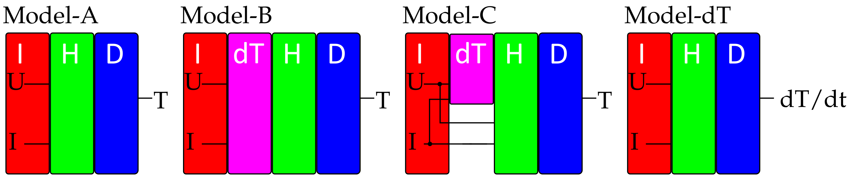
  • Hidden block (green) is a function of the number of hidden layers h lay and the number of neurons h neu . Each neuron is a LSTM neuron and each layer is fully connected as described in Section 2.2.
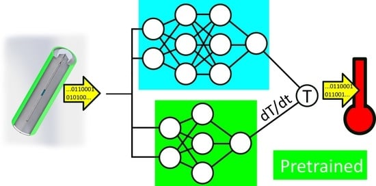
  • dT block (purple) is a fully trained LSTM model built as in Figure 7—Model-dT. It is structured like Model A; however, it was trained to predict the linear approximation d T cell / d t as calculated in Section 3.2.
  • Output block (blue) is a single LSTM neuron to bundle all the information coming from the hidden block.
The minimal time span necessary to predict a temperature value is depended on the window size h win . This means if h win = x the ANN will be able to make a prediction of T ( x ) based on the input values of I ( x h win ) to I ( x ) and U ( x h win ) to U ( x ) . In this study, three different model architectures are being investigated. The schematic of each model is represented in Figure 7. Model-A will function as the base model consisting of input-, hidden- and output blocks. Model-B has the same structure as Model-A except in-between the input block and hidden block is a fully trained dT block (Model-dT). Therefore, Model-B takes advantage of a form of artificial feature extraction, since the feature d T cell / d t ( t ) is not a product of how a model was trained, but has been trained in a controlled environment to produce d T cell / d t ( t ) . Model-C includes the dT block as well. However, the hidden block is being supplied with the information from the input block as well as the dT block.
Figure 8 illustrates an example of a model structure like Model-A or Model-dT. White neurons represent input neurons and yellow neurons represent LSTM neurons. Each neuron is fully connected to the upcoming layer. The background colors are analogous to Figure 7. This example uses three neurons for two layers in the hidden layer. The input and output structure is the same across all models. Model-B and Model-C have a fully trained dT-Model in-between input and hidden layer as described.
Five hyperparameters were investigated:
  • Window size h win : This is the number of data points the ANN will see at each time step. If the algorithm is supposed to estimate a temperature value for T ( 100 ) and h win = 10 , then the ANN would be fed T ( 89 ) T ( 99 ) . In order to make all architectures comparable, h win will only be dynamic at the base model (Model-A). For Model-B, -C and –dT, h win will be static. In case a value T ( x ) needs to be estimated with a window size h win = y with y > x , the data padding approach will be used [34]. This means, that the values will be automatically filled in to create an array with the appropriate dimensions.
  • Number of neurons h neu : This value represents the total number of neurons in the hidden block.
  • Number of hidden layers h lay : This is representative of the number of hidden layers in the hidden block. The number of neurons h npl of each individual layer l can be calculated by
    h npl ( l ) = h neu h lay , h neu h lay h neu h lay < l h lay h neu h lay + 1 , h neu h lay h neu h lay l h lay
    with h neu h lay and h lay l
  • Learning rate: During the backpropagation process, the weights are being adjusted according to Section 2.2. Learning rate h lear is the order of magnitude by which the weights are adjusted. A strong h lear is unlikely to find the optimal solution while a small h lear will make it challenging to reach a conclusion in a reasonable time frame. This is especially important when using an early stopping approach. In addition, this study uses an ADAM (derived from adaptive moment estimation) optimization algorithm to dynamically change the h lear during the training process [35].
  • Drop rate h drop : This parameter is meant to counteract overfitting by stochastically taking weights out of the equation. If we assume h drop = 0.1 , this would mean every neuron has a 10% chance of being bypassed.
To bypass the need for the number of training epochs n ep being yet another hyperparamter, a custom early-stopping approach has been integrated. If the training process is running for n ep > 10 , the training will stop if either τ loss ( n ep ) < τ loss ( 1 ) or if the slope a reg of
a reg = τ loss ( n ep ) ¯ n ep ¯ i = n ep 10 n ep ( n ep , i n ep ¯ ) ( τ loss ( n ep , i ) τ loss ( n ep ) ¯ ) i = n ep 10 n ep ( n ep , i n ep ¯ ) 2 ,
with
n ep ¯ = 1 10 i = n ep 10 n ep n ep , i ,
and
τ loss ( n ep ) ¯ = 1 10 i = n ep 10 n ep τ loss ( n ep , i ) ,
is positive.
To evaluate the models with individual hyperparameters, a constrained global optimization package built upon Bayesian inference and the Gaussian process were used. It attempts to find the maximum value of an unknown high cost function in as many few iterations as possible by adjusting the aforementioned hyperparameters [36]. It starts with a random grid search with n grid = 10 epochs. From there, the algorithm picks the best result as a starting point for the Bayesian optimization that runs for a maximum of n bays = 100 epochs. Because of the stochastic nature of ANN every iteration went through the training process twice and the arithmetic mean of the two error rates was calculated.

5. Results and Discussion

In this section, the results of all the models will be presented, compared and discussed. Table 1 shows the best results achieved in this experiment and is structured in the “Bayesian” and “Individual” areas. All models are trained to reduce τ train , and the hyperparamter h win is set static after the hyperparameter investigation of Model-A is completed as described in Section 3.
The area “Bayesian” is the arithmetic mean of the two results for the training loss τ train with the corresponding hyperparameters. Model-C was able to achieve the best results. To reduce the impact of the arithmetic mean, every individual model trained in “Bayesian” was investigated for “Individual”. Again, Model-C outperformed Model-A and Model-B.
The results shown in Table 1 are illustrated in Figure 9 for the training data set and Figure 10 for the validation data set.
Both figures show the predicted temperature values for the two models trained in the area “Bayesian” (“Bayesian #1” and “Bayesian #2”) and the overall best result in the area “Individual” for all models (Model-A, Model-B, Model-C and Model-dT) in contrast to the measured values (Ground Truth). In addition, each figure is subdivided into four areas (a)–(d).
These areas provide four enlarged views for a more detailed analysis on the training data in Figure 11 and validation data in Figure 12. The time span and position of all areas are identical to the areas in Figure 3 and Figure 5, respectively.
The success rate of the Model-dT is higher than predicting the absolute value. Calculating the linear approximation d T / d t as shown in Section 3.2 will amplify the noise produced by T cell . Figure 9 and Figure 10 show, that the ANN successfully performs a noise reduction and therefore, compresses the upper and lower limits. However, it filters out the information when heat is generated Q gen ( d T cell / d t ( t i ) > 0 ) and when heat is dissipated Q dis ( d T cell / d t ( t i ) < 0 ) . Thus, it aids Model-C to produce absolute values, which is to be taken as the key message of this research. Model-dT by itself is not sufficient to extrapolate the absolute values since every error is being summed up, resulting in a temperature drift which is not suitable for real life applications.
The predictions in Figure 9 show similar performance results to the predictions in Figure 10. Therefore, no signs of overfitting occurred.
The models do not aim to simply classify the sections in Section 3.2 and predict a mean value. Analyzing the enlarged sections (Figure 11a–d and Figure 12a–d) shows the models’ ability to learn the physical behavior of the LIBC. The model knows when T cell increases/decreases depending on the previous time step, and the active current load and voltage response that had been given in h win . Therefore, the model understands when the effects of Q gen or Q dis dominate.
Due to the limited amount of training data, not every situation gets a sufficient amount of attention. This is most notably when the LIBC heats up from T amb or cools down to T amb .
The “Individual” predictions perform visually the poorest of all graphs. This shows the importance of having more than one ANN trained with the same hyperparameter settings to reduce the effects of the stochastic nature.
The overall investigated temperature range is 24.53   ° C ± 0.01   ° C T cell 35.76   ° C ± 0.01   ° C . In this spectrum, Model-A achieved an accuracy of Δ T cell = 0.023   ° C during training and Δ T cell = 0.015   ° C during validation, Model-B Δ T cell = 0.064   ° C during training and Δ T cell = 0.043   ° C during validation and Model-C Δ T cell = 0.012   ° C during training and Δ T cell = 0.008   ° C during validation.
Model-B shows the poorest performance. This is most likely due to the dimensionality reduction. Where the input layer of Model-A has a dimension of two (U,I) and Model-C a dimension of three (U,I, d T cell / d t ( t i ) ), the hidden block in Model-B is only provided one dimension ( d T cell / d t ( t i ) ). Model-A and Model-C both show that the physical temperature behavior of a cell was learned. This is best illustrated in section (d) of Figure 11 and Figure 12. The LIBC can correctly predict the trend when to cool down and when to heat up based on the current inputs (U,I) and the previous cell states. Model-C outperformed Model-A and Model-B.

6. Conclusions and Future Work

The impact of artificial feature extraction using the first derivative in combination with ANN has been investigated. In this regard, the following steps have been taken to show its effectiveness:
  • A LIBC has been prepared with an internal NTC-temperature sensor with the aim to prevent a time delay from heat generation to heat dissipation.
  • A custom measuring system was designed to track the temperature and to synchronize the temperature data with the data of the battery system.
  • Using this approach, a training- and validation dataset was created to investigate three LSTM-architectures. A hyperparameter analysis for each model has been carried out to find the optimal model structure for each sub model. Model-A architecture is the base model, Model-B architecture uses an additional dT-layer, that has been separately trained to forecast the linear approximation of d T cell / d t ( t i ) and the third Model-C benefits from both approaches (Model-A and Model-B). Model-C was able to outperform Model-A and Model-B, which shows that artificial feature extraction is a useful method to improve model accuracy in the non-linear state of temperature prediction in LIBCs. This method made it possible to increase the accuracy by Δ T cell = 0.01   ° C for the training data and by Δ T cell = 0.007   ° C for the validation data compared to the base model with only the information of the current profile I and its corresponding voltage response U.
To show the full potential of data driven temperature prediction models for lithium-ion-battery systems, I would like to make the following suggestions for the data set used to train the model:
  • Broader temperature range;
  • Variable ambient temperature;
  • Implementing real life drive cycles.
In addition, the transferability needs to be looked at. That would include transferability between cell technologies and extrapolation from cell to module level. To compensate for the high computational effort to train an ANNs and the need for training data, a cloud server can be implemented, trying to find patterns across battery technologies and different topologies.

Author Contributions

M.K.: conceptualization, methodology, software, validation, formal analysis, investigation, writing—original draft, visualization; M.S.: conceptualization, writing—review and editing, supervision, validation; A.F.: writing—review and editing, validation; J.P.-B.: writing—review and editing; K.P.B.: conceptualization, writing—review and editing, supervision, funding acquisition. All authors have read and agreed to the published version of the manuscript.

Funding

This work was supported by Bundesministerium für Wirtschaft und Energie [19l21014D].

Institutional Review Board Statement

Not applicable.

Informed Consent Statement

Not applicable.

Data Availability Statement

The data presented in this study are available on request from the corresponding author.

Acknowledgments

I would like to thank the Bundesministerium für Wirtschaft und Energie for financial resources and the project management organisation TÜV Rheinland Consulting GmBH.

Conflicts of Interest

The authors declare no conflict of interest.

References

  1. Lyu, Y.; Siddique, A.; Hasibul Majid, S.; Biglarbegian, M.; Gadsden, S.; Mahmud, S. Electric vehicle battery thermal management system with thermoelectric cooling. Energy Rep. 2019, 5, 822–827. [Google Scholar] [CrossRef]
  2. Li, W.; Rentemeister, M.; Badeda, J.; Jöst, D.; Schulte, D.; Sauer, D.U. Digital twin for battery systems: Cloud battery management system with online state-of-charge and state-of-health estimation. J. Energy Storage 2020, 30, 101557. [Google Scholar] [CrossRef]
  3. Ma, S.; Jiang, M.; Tao, P.; Song, C.; Wu, J.; Wang, J.; Deng, T.; Shang, W. Temperature effect and thermal impact in lithium-ion batteries: A review. Prog. Nat. Sci. Mater. Int. 2018, 28, 653–666. [Google Scholar] [CrossRef]
  4. Yang, Y.; Huang, X.; Cao, Z.; Chen, G. Thermally conductive separator with hierarchical nano/microstructures for improving thermal management of batteries. Nano Energy 2016, 22, 301–309. [Google Scholar] [CrossRef] [Green Version]
  5. Cavalheiro, G.; Iriyama, T.; Nelson, G.; Huang, S.; Zhang, G. Effects of Non-Uniform Temperature Distribution on Degradation of Lithium-Ion Batteries. J. Electrochem. Energy Convers. Storage 2019, 17, 021101. [Google Scholar] [CrossRef]
  6. Fill, A.; Avdyli, A.; Birke, K.P. Online Data-based Cell State Estimation of a Lithium-Ion Battery. In Proceedings of the 2020 2nd IEEE International Conference on Industrial Electronics for Sustainable Energy Systems (IESES), Cagliari, Italy, 1–3 September 2020; Volume 1, pp. 351–356. [Google Scholar] [CrossRef]
  7. Guo, G.; Long, B.; Cheng, B.; Zhou, S.; Xu, P.; Cao, B. Three-dimensional thermal finite element modeling of lithium-ion battery in thermal abuse application. J. Power Sources 2010, 195, 2393–2398. [Google Scholar] [CrossRef]
  8. Spinner, N.S.; Love, C.T.; Rose-Pehrsson, S.L.; Tuttle, S.G. Expanding the Operational Limits of the Single-Point Impedance Diagnostic for Internal Temperature Monitoring of Lithium-ion Batteries. Electrochim. Acta 2015, 174, 488–493. [Google Scholar] [CrossRef]
  9. Raijmakers, L.; Danilov, D.; Lammeren, J.; Lammers, M.; Notten, P. Sensorless Battery Temperature Measurements Based on Electrochemical Impedance Spectroscopy. J. Power Sources 2013, 247, 539–544. [Google Scholar] [CrossRef]
  10. Wang, S.; Fernandez, C.; Yu, C.; Fan, Y.; Cao, W.; Stroe, D.I. A novel charged state prediction method of the lithium ion battery packs based on the composite equivalent modeling and improved splice Kalman filtering algorithm. J. Power Sources 2020, 471, 228450. [Google Scholar] [CrossRef]
  11. Thomas, K.E.; Newman, J. Thermal Modeling of Porous Insertion Electrodes. J. Electrochem. Soc. 2003, 150, A176. [Google Scholar] [CrossRef]
  12. Zhang, J.; Huang, J.; Li, Z.; Wu, B.; Nie, Z.; Sun, Y.; An, F.; Wu, N. Comparison and validation of methods for estimating heat generation rate of large-format lithium-ion batteries. J. Therm. Anal. Calorim. 2014, 117, 447–461. [Google Scholar] [CrossRef]
  13. Au Severson, K.A.; Attia, P.M.; Jin, N.; Perkins, N.; Jiang, B.; Yang, Z.; Chen, M.H.; Aykol, M.; Herring, P.K.; Fraggedakis, D.; et al. Data-driven prediction of battery cycle life before capacity degradation. Nat. Energy 2019, 4, 383–391. [Google Scholar] [CrossRef] [Green Version]
  14. Yang, F.; Li, W.; Li, C.; Miao, Q. State-of-charge estimation of lithium-ion batteries based on gated recurrent neural network. Energy 2019, 175, 66–75. [Google Scholar] [CrossRef]
  15. Li, P.; Zhang, Z.; Xiong, Q.; Ding, B.; Hou, J.; Luo, D.; Rong, Y.; Li, S. State-of-health estimation and remaining useful life prediction for the lithium-ion battery based on a variant long short term memory neural network. J. Power Sources 2020, 459, 228069. [Google Scholar] [CrossRef]
  16. Kleiner, J.; Stuckenberger, M.; Komsiyska, L.; Endisch, C. Real-time core temperature prediction of prismatic automotive lithium-ion battery cells based on artificial neural networks. J. Energy Storage 2021, 39, 102588. [Google Scholar] [CrossRef]
  17. Feng, F.; Teng, S.; Liu, K.; Xie, J.; Xie, Y.; Liu, B.; Li, K. Co-estimation of lithium-ion battery state of charge and state of temperature based on a hybrid electrochemical-thermal-neural-network model. J. Power Sources 2020, 455, 227935. [Google Scholar] [CrossRef]
  18. Zhu, S.; He, C.; Zhao, N.; Sha, J. Data-driven analysis on thermal effects and temperature changes of lithium-ion battery. J. Power Sources 2021, 482, 228983. [Google Scholar] [CrossRef]
  19. Wu, B.; Han, S.; Shin, K.G.; Lu, W. Application of artificial neural networks in design of lithium-ion batteries. J. Power Sources 2018, 395, 128–136. [Google Scholar] [CrossRef]
  20. Zhu, C.; Li, X.; Song, L.; Xiang, L. Development of a theoretically based thermal model for lithium ion battery pack. J. Power Sources 2013, 223, 155–164. [Google Scholar] [CrossRef]
  21. Rao, L.; Newman, J. Heat-Generation Rate and General Energy Balance for Insertion Battery Systems. J. Electrochem. Soc. 1997, 144, 2697–2704. [Google Scholar] [CrossRef]
  22. Abdul-Quadir, Y.; Laurila, T.; Karppinen, J.; Jalkanen, K.; Vuorilehto, K.; Skogström, L.; Paulasto-Kröckel, M. Heat generation in high power prismatic Li-ion battery cell with LiMnNiCoO2 cathode material. Int. J. Energy Res. 2014, 38, 1424–1437. [Google Scholar] [CrossRef]
  23. Bandhauer, T.; Garimella, S.; Fuller, T. A Critical Review of Thermal Issues in Lithium-Ion Batteries. J. Electrochem. Soc. 2011, 158, R1. [Google Scholar] [CrossRef]
  24. Thomas, K.E.; Newman, J. Heats of mixing and of entropy in porous insertion electrodes. J. Power Sources 2003, 119–121, 844–849. [Google Scholar] [CrossRef]
  25. Chen, S.; Wan, C.; Wang, Y. Thermal analysis of lithium-ion batteries. J. Power Sources 2005, 140, 111–124. [Google Scholar] [CrossRef]
  26. Keil, P.; Jossen, A. Thermal FDM Battery Model. In Proceedings of the 2020 Advanced Battery Power–Kraftwerk Batterie, Münster, Germany, 23–25 March 2012. [Google Scholar]
  27. Dongare, A.; Kharde, R.R.; Kachare, A.D. Introduction to Artificial Neural Network. Int. J. Eng. Innov. Technol. (IJEIT) 2012, 2, 189–194. [Google Scholar]
  28. Lipton, Z. A Critical Review of Recurrent Neural Networks for Sequence Learning. arXiv 2015, arXiv:1506.00019. [Google Scholar]
  29. Bird, J.; Ekart, A.; Buckingham, C.; Faria, D. Evolutionary Optimisation of Fully Connected Artificial Neural Network Topology. In Proceedings of the SAI Computing Conference 2019, Las Vegas, NV, USA, 25–26 April 2019. [Google Scholar]
  30. Rumelhart, D.E.; McClelland, J.L. Learning Internal Representations by Error Propagation. In Parallel Distributed Processing: Explorations in the Microstructure of Cognition; Foundations MIT Press: Cambridge, MA, USA, 1987; pp. 992–997. [Google Scholar]
  31. Yu, Y.; Si, X.; Hu, C.; Zhang, J. A Review of Recurrent Neural Networks: LSTM Cells and Network Architectures. Neural Comput. 2019, 31, 1235–1270. [Google Scholar] [CrossRef]
  32. Hochreiter, S.; Schmidhuber, J. Long Short-Term Memory. Neural Comput. 1997, 9, 1735–1780. [Google Scholar] [CrossRef]
  33. Ruan, H.; Sun, B.; Jiang, J.; Zhang, W.; He, X.; Su, X.; Bian, J.; Gao, W. A modified-electrochemical impedance spectroscopy-based multi-time-scale fractional-order model for lithium-ion batteries. Electrochim. Acta 2021, 394, 139066. [Google Scholar] [CrossRef]
  34. Dwarampudi, M.; Reddy, N.V.S. Effects of padding on LSTMs and CNNs. arXiv 2019, arXiv:1903.07288. [Google Scholar]
  35. Kingma, D.; Ba, J. Adam: A Method for Stochastic Optimization. In Proceedings of the International Conference on Learning Representations, Banff, AB, Canada, 14–16 April 2014. [Google Scholar]
  36. Nogueira, F. Bayesian Optimization: Open Source Constrained Global Optimization Tool for Python. Available online: https://github.com/fmfn/BayesianOptimization (accessed on 9 June 2021).
Figure 1. LIBC equipped with temperature sensor. On the left is a photograph of the prepared cell. On the left is a sectional view of sensor placement in LIBC. The figure shows the production-related cavity with an NTC-sensor placed in the middle. The cavity is accessed by a through-hole in the center of the negative terminal.
Batteries 08 00036 g001
Figure 2. Nyquist plot of the EIS measurement carried out before (Pre) and after (Post) the LIBC was equipped with a temperature sensor. Point (a) and (b) compare the two high points of the first semi-circle.
Batteries 08 00036 g002
Figure 3. Selected data to train the algorithm. Presented are four subfigures showing temperature response T cell ( t train ) , temperature change over time d T cell / d t ( t train ) , current profile I ( t train ) and voltage response U ( t train ) . Four areas are marked (ad).
Batteries 08 00036 g003
Figure 4. Enlarged view of the areas marked in Figure 3. Presented are temperature response T cell ( t train ) and current profile I ( t train ) of each of the marked ares (ad).
Batteries 08 00036 g004
Figure 5. Selected data to test the algorithm. Presented are four subfigures showing temperature response T cell ( t test ) , temperature change over time d T cell / d t ( t test ) , current profile I ( t test ) and voltage response U ( t test ) . Four areas are marked (ad).
Batteries 08 00036 g005
Figure 6. Enlarged view of the areas marked in Figure 5. Presented are temperature response T cell ( t test ) and current profile I ( t test ) of each of the marked ares (ad).
Batteries 08 00036 g006
Figure 7. Layer schematic of different models. I-block (red) is the input layer, H-block (green) the hidden layer, D-block (blue) the output layer and dT-block (purple) summarizes the pre trained Model-dT.
Batteries 08 00036 g007
Figure 8. Example of a single model like Model-A or Model-dT with two inputs (Input 1 and Input 2) and one output (Output). White neurons represent input neurons and yellow neurons represent LSTM neurons.
Batteries 08 00036 g008
Figure 9. Predicted values of all models in four subfigures are given for the training data set. Model-A to Model-C show ground truth, Bayesian #1, Bayesian #2 and the most promising individual results. Model-dT illustrates ground truth and the predicted values of the dT-Model. Four areas are marked from (ad).
Batteries 08 00036 g009
Figure 10. Predicted values of all models in four subfigures are given for the testing data set. Model-A to Model-C show ground truth, Bayesian #1, Bayesian #2 and the most promising individual results. Model-dT illustrates ground truth and the predicted values of the dT-Model. Four areas are marked from (ad).
Batteries 08 00036 g010
Figure 11. Predicted values of all models in four subfigures are given for the training data set. Model-A to Model-C show ground truth, Bayesian #1, Bayesian #2 and the most promising individual results. Model-dT illustrates ground truth and the predicted values of the dT-Model. Four areas are marked from (ad).
Batteries 08 00036 g011
Figure 12. Predicted values of all models in four subfigures are given for the testing data set. Model-A to Model-C show ground truth, Bayesian #1, Bayesian #2 and the most promising individal results. Model-dT illustrates ground truth and the predicted values of the dT-Model. Four areas are marked from (ad).
Batteries 08 00036 g012
Table 1. Hyperparameter results. The table shows the hyperparameter configuration for the hyperparameters h win , h lay , h neu , h drop and h learn for each model. The “Bayesian” area shows the arithmetic mean of two results with the same hyperparameter configuration and “Individual” area shows the results for each individual model.
Model τ train h win h lay h neu h drop h learn
A 9.02 × 10 3 825 0.0670 4.23 × 10 6
BayesianB 5.48 × 10 2 815 0.0818 1.72 × 10 6
C 7.44 × 10 3 815 0.0876 8.95 × 10 6
A 2.05 × 10 3 10128 0.0419 6.88 × 10 6
IndividualB 5.73 × 10 3 8124 0.0687 8.36 × 10 6
C 1.04 × 10 3 8182 0.0373 2.12 × 10 5
Publisher’s Note: MDPI stays neutral with regard to jurisdictional claims in published maps and institutional affiliations.

