Article

Online Identification of VLRA Battery Model Parameters Using Electrochemical Impedance Spectroscopy

by
Javier Olarte
1,2,
Jaione Martinez de Ilarduya
1,
Ekaitz Zulueta
2,*,
Raquel Ferret
1,
Joseba Garcia-Ortega
2 and
Jose Manuel Lopez-Guede
2
1
Centre for Cooperative Research on Alternative Energies (CIC EnergiGUNE), Basque Research and Technology Alliance (BRTA), Alava Technology Park, Albert Einstein 48, 01510 Vitoria-Gasteiz, Álava, Spain
2
Department of Systems and Automatic Control, Faculty of Engineering of Vitoria-Gasteiz, University of the Basque Country (UPV/EHU), Nieves Cano, 01006 Vitoria-Gasteiz, Álava, Spain
*
Author to whom correspondence should be addressed.
Batteries 2022, 8(11), 238; https://doi.org/10.3390/batteries8110238
Submission received: 29 August 2022 / Revised: 13 October 2022 / Accepted: 27 October 2022 / Published: 14 November 2022
(This article belongs to the Special Issue Feature Papers to Celebrate the First Impact Factor of Batteries)

Abstract

:
This paper introduces the use of a new low-computation cost algorithm combining neural networks with the Nelder–Mead simplex method to monitor the variations of the parameters of a previously selected equivalent circuit calculated from Electrochemical Impedance Spectroscopy (EIS) corresponding to a series of battery aging experiments. These variations could be correlated with variations in the battery state over time and, therefore, identify or predict battery degradation patterns or failure modes. The authors have benchmarked four different Electrical Equivalent Circuit (EEC) parameter identification algorithms: plain neural network mapping EIS raw data to EEC parameters, Particle Swarm Optimization, Zview, and the proposed new one. In order to improve the prediction accuracy of the neural network, a data augmentation method has been proposed to improve the neural network training error. The proposed parameter identification algorithms have been compared and validated through real data obtained from a six-month aging test experiment carried out with a set of six commercial 80 Ah VLRA batteries under different cycling and temperature operation conditions.

1. Introduction

Among the most common battery characterization methods, we find energy counting, open circuit voltage, and electrochemical impedance spectroscopy. Techniques based on open circuit voltage are, undoubtedly, a line of great interest and applicability for many battery applications as reflected in multiple works [1,2,3,4] but require a long time to diagnose or are, sometimes, not able to be used for practical reasons. Online monitoring of the Electrochemical Impedance Spectroscopy (EIS) undoubtedly allows the adjustment and improvement of the certainty of battery state estimation as several works point out [5,6,7,8,9,10]. This paper focuses on a method to online monitor the variations of parameters of a previously selected equivalent circuit calculated from EIS datasets corresponding to a series of battery aging experiments in line with the research lines of Muraiu et al. [11] which identifies correlations between State of Health (SOH) conditions and some parameters of a given equivalent circuit best fitted for the battery under testing. Although the proposed algorithms have been validated with VLRA batteries, they can also be used with lithium-ion batteries, as suggested by several recent works [12,13,14] using this technique for identification and diagnosis of battery degradation modes.
Experiments involving the characterization of a battery for a given case of use require specific laboratory equipment and experienced personnel and may take several months. Once the characterization process has been done, designing the optimum real-time battery monitoring system is a second challenge, where the use of EIS sensors at cell level facilitates the continuous monitoring of SOH of the battery [15,16]. It is at this point that the development of algorithms based on innovative models related to artificial intelligence allows for innovative battery health and capacity estimation models.
Among the various artificial intelligence and machine learning techniques, neural networks have been extensively used in the development of both data-driven and empirical models for battery diagnosis and prognosis, as reported by Lombardo et al. [17], where EIS appears as a very promising technique for obtaining even more precise online estimation models for aging and health prediction.
Indeed, EIS data are very powerful tools for identifying battery electrical equivalent circuit models since they help in evaluating different battery states and in operando conditions as demonstrated by Kwiecien et al. [18] and other researchers [19,20,21,22]. Usually, the identification of the electrical equivalent circuit parameters to be extracted from EIS requires human expertise complementary to aided support specific software such as Zview, which offers impedance/gain phase graphing tools and guided circuit selection advice, as seen in the study realized by Csomós et al. [23].
The selection of appropriate Electrical Equivalent Circuit (EEC) is fundamental to the use of EIS-based SOH estimation methods, which must also take full account of the impact of temperature and SOC on the models as also reported by Wang et al. [24].
In this paper, the authors have applied neural networks in parameter identification due to their capability to create and match nonlinear relationships between inputs (EIS data) and outputs (parameters of the equivalent circuit) as one of the benchmarked algorithms, as in the case of Chun et al. [25]. Jiménez-Bermejo et al. have also used them to obtain a more accurate battery SOC estimation for electric vehicles [26], and Yang et al. [27] have used BP neural networks for the proper estimation of a battery SOH in electric vehicles, in which they used a large amount of experimental data to feed the neural network (NN). However, neural networks need extensive training data sets. Obtaining experimental data for all battery-operating conditions is highly time-consuming, so the authors propose training the neural network with an initial set of experimental EIS data plus a second set of augmented synthetic data corresponding to variations of the experimental values for the equivalent circuit model as a means of minimizing the neural network training error. This data augmentation, however, must be generated in a very careful way since EIS parameters are very dependent on each other. The authors propose an innovative data generation method where the new data has the impact of reducing the learning error of the neural network without affecting the final error of estimation of the equivalent electrical circuit parameters.
Taking into account the need to start from experimental data to train the neural networks, Capizzi et al. [28] have used recurrent NN to model the charge and discharge voltage curves of lead acid batteries.
Another very interesting study based on neural networks is Young et al. [29], which trains the networks with float voltage, specific gravity, and water addition electrolyte level data as estimators of battery performance. On the other hand, Morita [30] proposed estimating the SOC from observable data with a preprocess involving the calculation of intermediate variables of an equivalent model, specifically with the polarization index, which allowed a substantial improvement of the estimation accuracy.
The authors propose an automatic way to identify all the parameters of an equivalent circuit in a selected battery by taking a series of EIS data using a previously trained NN whose output parameters are used as inputs to the simplex optimization algorithm.
The method is similar to that described by Lagarias et al. in [31], which generates the final values of the equivalent circuit parameters. Once the NN is trained, an algorithm with very low computational cost can be implemented, allowing for the design of systems useful for monitoring the evolution of the equivalent circuit parameters associated with the battery.
In a previous work, the authors already reported a two-step parameter identification algorithm [32] in order to monitor variations of the EEC parameters, whereas, in this new work, the target is to make a more rigorous comparison with other known methods while identifying new algorithms that offer low computational costs. Additionally, the objective motivating this new hybrid approach is to find a new and more accurate automatic identification of EEC parameters from raw EIS data. Although there are many works in the literature that use NN to estimate SOC and SOH values, we have not found any work similar to the approach of this paper where the NN is used as an estimator of the initial values or input parameters to initialize a second algorithm, in this case the Nelder–Mead simplex method.
The proposed hybrid algorithm, together with the augmentation data method, proves a significant enhancement in the identification accuracy as compared to a plain NN mapping EIS raw data and the EEC parameters algorithm, the Particle Swarm Optimization algorithm or Zview.
The authors’ ultimate goal with the proposed method is to automatically online monitor variations in the equivalent circuit parameters in operation with low-cost impedance sensors that allow for the induction of variations in battery health status or failure modes from the electrochemical interpretation of these values.
Although the validation of the proposed algorithm tests has been carried out with lead batteries, the methodology is valid for other electrochemicals currently more in vogue such as lithium where there are many works that rely on models based on the interpretation of equivalent electrical circuits as shown in the work of Lidiya Komsiyska et al. [33].
The paper structure is as follows. Materials and methods, that is, the experimental setup and the EEC selection are given in Section 2. Section 3 presents the algorithms benchmarked with more details related to the neural network data augmentation algorithm, the parameter identification process, and the validation and test of the selected neural network. Section 4 offers a discussion of the results. Finally, in Section 5 some main conclusions can be found, as well as possible directions of future developments.

2. Materials and Methods

2.1. Experimental Setup and Battery Testing Protocol

The data used for this work is based on a set of six 12 V 80 Ah high temperature lead-acid batteries, aged for six months under different cycling and temperature operation conditions.
These batteries had improved performances at high temperatures, when compared with standard lead-acid batteries. They included an anode composed of lead (Pb), while the cathode consisted of a paste of lead oxide (PbO2). The electrodes were separated by a porous separator impregnated with an electrolyte containing an aqueous acid solution of H2SO4. Electrochemical data of the performed experiments were gathered by means of Arbin potentiostat, and the EIS measurements were recorded by means of a Gamry 3000 battery tester.
The ageing was carried out at different temperatures and charge/discharge duty cycles. From these accelerated ageing tests, parameters/signals of the electrochemical system were extracted for later use with the benchmarked identification algorithms. The testing protocol included the Constant-Current (CC) charge stage and the Constant-Voltage (CV) charge stage up to 2.35 V/cell in each lead acid battery, while the discharge process was carried out up to 1.8 V/cell. Periodic impedance measurements were performed at different SOC levels (0%, 20%, 40%, 60%, 80%, and 100%). At each SOC level, 12 h of relaxation was established before performing the impedance measurement, which was performed under an excitation current of 50 mA and in a frequency range from 10 mHz to 10 kHz. In this way, impedance spectra were obtained at different states of charge in the batteries at different aged conditions and from the same manufacturer.
Figure 1 shows four Nyquist plots selected from the EIS experimental data, namely at 25 °C and 50 °C with SOC values of 100% and 20% for new and degraded cells. As an example, the axes of dispersion in temperature, SOC and SOH values are illustrated. Although it is not the purpose of this work to identify in detail the causal relationships, the figure and the parameter values clearly demonstrate that it is possible to identify variations of the parameters for different operating states of the lead acid battery. It is from this point onwards that it is proposed to identify an equivalent circuit model that can be fitted to the different Nyquist pattern diagrams with the lowest mean error for all conditions tested.

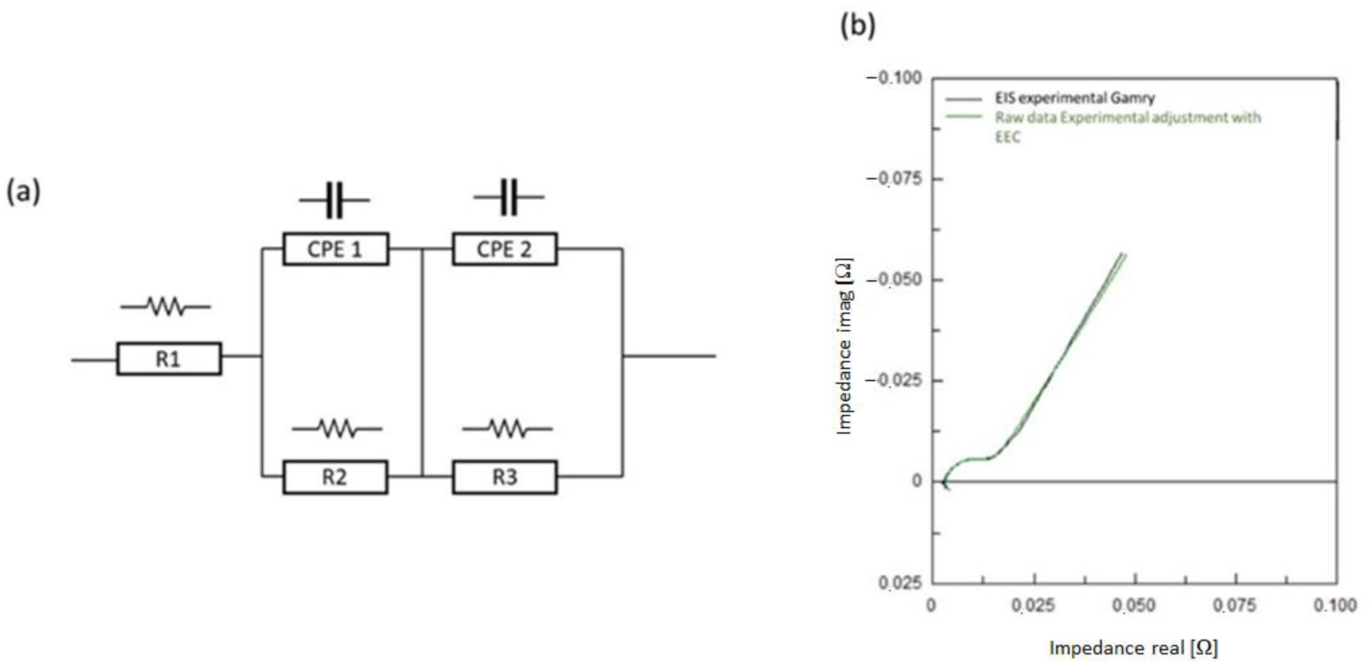
2.2. Battery Characterization and EEC Selection

The EIS extracted from the tests were analyzed in order to specify an EEC model. This step let the authors extract the parameters of the model that must be identified. Figure 2a illustrates the equivalent circuit model proposed by the authors for all of the experiments in this article. Constant phase elements were employed to determine this EEC, in order to adjust the experimental data. An electrode’s non-ideal capacitive behaviors were taken into account; therefore, a constant phase element (CPE) was used. This CPE is a capacitor whose α parameter represents the leakage. This element becomes a pure capacitor when α is equal to 1 [24]. A CPE element was selected instead of a Warburg one since the latter, at lower frequencies, does not support the fitting of impedance spectra for lower SOC levels (0% SOC). The independent variables such as ohmic resistance, R2, R3, CPE1-T, CPE1-P, CPE2-T, CPE2-P, and their variations were manually extracted by Zview software from the adjustment (Figure 2b).
Table 1 shows the EEC parameters values (R1, R2, R3, CPE1-T, CPE1-P, CPE2-T, and CPE2-P) fitted to the selected EEC (see Figure 2b) using the Zview software. Figure 2b presents both the EIS experimental data selected from the Gamry instrument (black line) and the EEC fitting (green line). These reference parameters are taken into account to generate the augmented data.
According to the proposed equivalent electric circuit for the adjustment of the experimental data, the following equations must be applied to develop the EIS augmented data to train the neuronal network, taking into account the R1, R2, R3, CPE1-T, CPE1-P, CPE2-T, and CPE2-P parameters. Equations (1) and (2) show the fundamental significance of the parameters i and ω.
i = 1
w = 2 · π · f
Equations (3)–(7) show the significance of the different parameters in the expression of impedance adjustment.
Z c p e 1 = 1 c p e t 1 ·   ( i · w ) c p e p 1
Z c p e 2 = 1 c p e t 2 ·   ( i · w ) c p e p 2
Z c p e 1 R 2 = Z c p e 1 ·   R 2 Z c p e 1 + R 2
Z c p e 2 R 3 = Z c p e 2 ·   R 3 Z c p e 2 + R 3
Z b a t t e r y = R 1 + L 1 · i · w + Z c p e 1 R 2 + Z c p e 2 R 3

3. Design Methodology

In this section, we briefly present the three identification algorithms benchmarked versus the NN with Nelder–Mead algorithm that is described with more detail in Section 3.4.
The more important highlight is the combination of both methods: neural networks for the first identification step and the fine identification step with simplex method for faster convergence. The authors have suggested making the first identification step with neural networks and not with PSO or other swarm optimization algorithms because swarm optimization algorithms must make many trial and errors until they reach a good identification parameter set before the second identification step. The neural network makes this process during training; therefore, the neural network makes the first identification process with trained knowledge and obtains results immediately. On the contrary, swarm optimization algorithms make the first identification process without any trained knowledge because they always start with random parameter sets.
When a weights-based identification algorithm identifies circuit parameters, the parameter related to the biggest weights frequency samples are better identified than other parameters. In some cases, this approach could be good if it is clear which parameter is the most relevant for a given application. In this case, the algorithm gives the same importance to all frequencies, in order to identify all the parameters based on the whole frequency range in order to identify whole parameters with the same importance.

3.1. Zview Algorithm

A human expert assisted by Zview software uses the least-squares fit method in which the human expert supplies the initial value of the identified circuit parameters. Zview algorithms provide different options in order to apply a least-square error method to reduce the cost function given in Equation (8). The maximum optimization iterations number is set to 100. The cost function proposed in Equation (8) takes into account the module of error between the measured experimental EIS and the model’s theoretical EIS. This error has complex values for different frequencies. In this study, the cost evaluates the error’s squared modules. Thus, the cost function has a real value.
J = 1 2 · N s a m p l e s · i = 1 u = N s a m p l e s | | Z b a t t e r y t h e o ( P w i ) Z b a t t e r y e x p ( w i ) | | 2

3.2. Neural Network Algorithm

In this case, the authors have trained a NN to map the EIS data (inputs: the EIS impedance values at 121 different frequencies, from 0.01 Hz to 10 kHz) to the EEC parameters (outputs: R1, R2, R3, CPE1-T, CPE1-P, CPE2-T, and CPE2-P). The artificial neural network takes the experimental EIS measures for different frequencies and then returns the EEC parameters of the equivalent circuit. Therefore, the artificial neural network needs a set of EIS spectrum as training patterns, as well as its corresponding EIS equivalent circuits’ parameters. In order to calculate the electrical equipment parameters from a measured electrochemical impedance spectroscopy, the authors propose a feed-forward neural network fed by augmented data generated from a small amount of manually adjusted EIS experimental data. This NN consists of a series of layers, with the first one being the input layer (mapped to the EIS data) and the last one being the output layer (mapped to the EEC parameters). We proposed training one neural network for each parameter, i.e., seven networks corresponding to the seven parameters of the selected equivalent circuit.

3.3. PSO Algorithm

The third algorithm is based on the Particle Swarm Optimization (PSO) algorithm, and the authors have applied its standard version [23]. We used the following: constant inertia weights set to 0.1, max exploration coefficient φ1 set to 0.1, max exploitation coefficient φ2 set to 0.1, the number of particles set to 5, and the time integration constant set to 1. The algorithm’s maximum number of iterations is 500. In order to have a good convergence time, the authors have limited the number of particles to 5 because the search space dimension (the number of identified parameters: R1, R2, R3, CPE1-T, CPE1-P, CPE2-T, and CPE2-P) is large.

3.4. Neural Network with Nelder-Mead Algorithm

Finally, a neural network combined with the Nelder–Mead Simplex [31] method is suggested. There are several algorithms that minimize the square values of a cost function. Actually, scientific programming languages like Matlab or Python (through module like scipy) apply different alternatives. On the one hand, Matlab applies the Nelder–Mead optimization algorithm. On the other hand, Python-Scipy applies different algorithms (for example, dogleg and the Region reflective algorithm or Levenberg–Marquand algorithm). All these algorithms achieve good results when initial values are near the global optimal point. Unfortunately, the authors needed an algorithm that automatically matches the EIS experimental spectrum without initial values for the EIS equivalent circuit’s parameters. The authors have chosen the Nelder–Mead algorithm because it is widely applied in optimization problems like system parameter identification. The Nelder–Mead algorithm has been set with standard values (reflection coefficient: ρ = 1, expansion coefficient: χ = 2, contraction coefficient: γ = ½, and shrinkage coefficient: σ = 1/2), with 1600 as the maximum iterations number, with 10−4 tolerance for cost function value and 10−4 tolerance for optimization variable (in this case, the tolerance of each identified circuit parameter). The method of generating the augmented data and the training process of the neural networks that generate the initialization values of the Nelder–Mead algorithm is detailed hereafter.

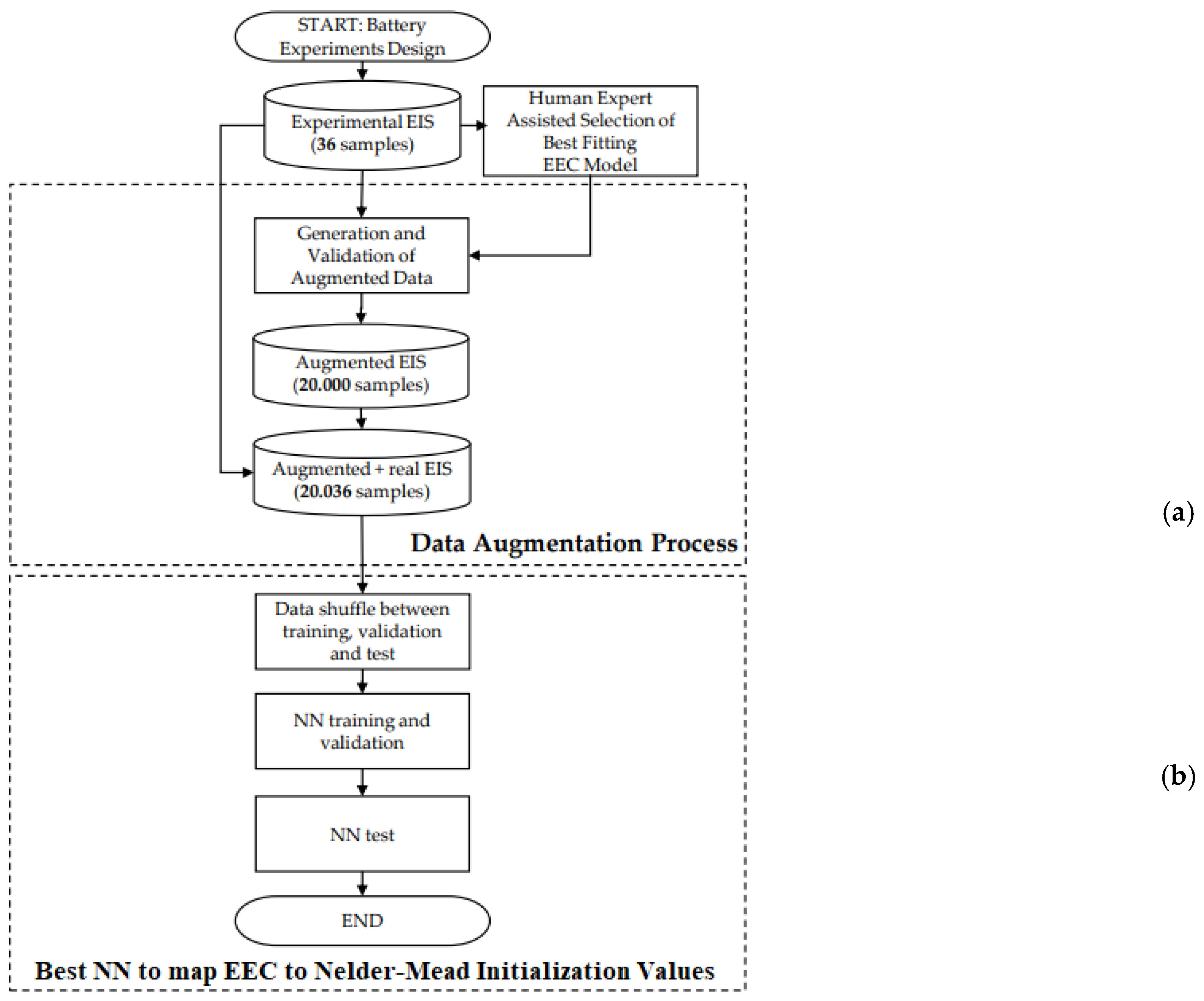
3.4.1. Experiment-Based Data Augmentation

Figure 3 identifies the main phases of the overall NN generation process, and Figure 4 further details the flowchart used for the data augmentation.
Using the experimental data obtained during the aging process, Nyquist diagrams were auto-generated from EIS, obtaining complementary augmented data via the following algorithmic random data-generation process. Given a log file of the experimental values corresponding to 20%, 40%, 60%, 80%, and 100% of the SOC battery status and using its minimum and maximum values for each parameter (R1, R2, R3, CPE1-T, CPE1-P, CPE2-T, and CPE2-P), a random value was generated per parameter. Therefore, the authors automatically generate several pseudorandom values. In order to guarantee that the augmented data do not negatively affect the estimation error of the proposed algorithm, only values between the maximum and minimum limits of the real spectra of the tests have been used, and, on the other hand, in the final validation of the algorithms, the networks that generate the lowest errors have been selected with the validation data against real spectra obtained from the characterization tests, which has shown that the augmented data have a positive impact on minimizing the training error of the neural networks, but not on the final error.
These values are generated via human expert guided identification parameter values. The minimum and maximum values are chosen following these estimated parameter values. The main objective is to augment the training data with a possible parameter value set. In order to assure that the augmented data is possible, the authors compared the EIS spectra that generates this parameter set with the experimental data.
With these generated parameters, the EIS was calculated and compared with its experimental counterpart, measuring the Mean Square Error (MSE). If it was not superior to a selected value (50% in this case), the circuit was accepted and the Nyquist diagram was plotted; otherwise, another round of parameters was randomly generated, until the MSE became acceptable. The MSE error (J) was calculated as shown below in Equation (8):
The process illustrated in Figure 5 was repeated as many times as required until the target samples met the acceptance MSE value. Every circuit with an acceptable MSE was saved for the next part of the process, which is training the neural network.

3.4.2. Training, Validation and Testing of the Neural Network Trained with Augmented Data

In order to evaluate the training of the seven neural networks (to identify each of the seven Nelder–Mead simplex parameters needed to calculate the EIS: R1, R2, R3, CPE1-T, CPE1-P, CPE2-T, and CPE2-P) using the augmented data generated from the experimental data, multiple neural networks were trained with different running conditions, namely by modifying the number of neurons and epochs.
Out of the complete set of experimental and augmented data set (20,036 equivalent circuits), 70% was used for neural network training, 15% was used for neural network validation and the remaining 15% for testing of the neural network.
All trained networks were one-hidden-layer neural networks. The selection of a single intermediate layer was decided on the basis of initial trials where networks were trained with more intermediate layers and where it was observed that no better results or accuracies were obtained and that training times were much longer and, in some cases, convergence in the training process was not achieved. In order to select the number of neurons in the networks, the authors performed different trials. The authors selected the best NN architecture. The results obtained in this process are explained in Section 4. The hidden layer neurons’ activation function is a sigmoid one. The number of maximum epochs and the maximum validation fail number are set in order to achieve good validation results. Notice that the full set of real and augmented data were only used to train the intermediate NN estimators of the initialization values of the Nelder process, but the 36 real data was finally use for the benchmark of the compared algorithms.

4. Results and Discussion

The process of training and selection of the best performing neural network and the comparison of the algorithms is presented in this section.

4.1. Neural Network Training and Validation

For the first experiment, a neural network of 10 neurons was trained during 100 epochs. The results are illustrated in Figure 6, Figure 7, Figure 8 and Figure 9. In Figure 6, the average error is acceptably close to zero. The error in Figure 6, Figure 7, Figure 8 and Figure 9 represents mean square error made on circuits parameters, during the artificial neural network’s training. These mean square error values are plotted in a histogram. The mean square error of the loss training function is calculated over the number of parameters of the circuit. Moreover, the training algorithm averages the mean square error over the number of training patterns. Then, no validation errors are perceived in the training state graph. Furthermore, high R correlation coefficient values are achieved on all of the examined datasets at 0.999. Finally, no outliers are found. Therefore, the model explains all data without making any extreme error. Hence, the variance in errors is very low. The training algorithm stopped at the maximum of 100 epochs.
In the second experiment, the maximum number of epochs was set to 200, maintaining 10 neurons, to assess whether the error reduced its medium value, a circumstance that is fulfilled. The main change seen in this case, compared to the previous one, is the error histogram, as the average error is now even closer to zero than before (Figure 7). This value results from the increment in the epoch quantity, as the network has more cycles to train. The remaining plots show very little change, so they are not included in the paper.
It is clear that, the more layers an artificial network has, the easier fitting the data becomes; however, complex neural networks equal more overfitting problems. In addition, adding more neurons per layer usually makes it easier to understand the different features that a neural network learns, in comparison with increasing the amount of layers the network has. In our proposal, there is only one hidden layer, which learns a specific input pattern. This property makes the neural network more interpretable. Moreover, the universal approximation theorem states that any square function integrable in a domain, can be approximated as well as needed with only one width hidden layer [34].
Thus, in the third experiment, the number of neurons was reduced to 5 while the maximum epochs or iterations was maintained at 100 in order to appropriately compare the results with those obtained in the first experiment. In Figure 8, we can clearly observe that the average error increases, indicating slightly worse but still acceptable results from the training.
For the fourth and last experiment, the neuron quantity was increased up to 20 and the epoch number was maintained at 100 to assess whether the pattern identified in earlier experiments was repeated in these/later ones. As expected, by increasing the number of neurons, the error was reduced (Figure 9).
Table 2 summarizes the results corresponding to the four experiments. The proposed neural networks show a low error interval in all cases when compared with one another, suggesting that the estimated results are precise. The peak values are reached with the 20-neuron network at 100 epochs being slightly better than the results reached with the 10-neuron network at 200 epochs. In Table 2, the authors summarize the different training experiments performed. The conclusion reached is that the optimum case is one in which the resulting layers with 10 neurons and 200 epoch shows a sigmoid activation function. Storing the connection weights in smaller networks is less resource intensive and, furthermore, can be implemented in hardware more efficiently. In fact, each iteration of the training of a smaller network takes less time and memory compared with bigger networks. Therefore, as the 10-neuron network achieves acceptable results, the other cases have been discarded.

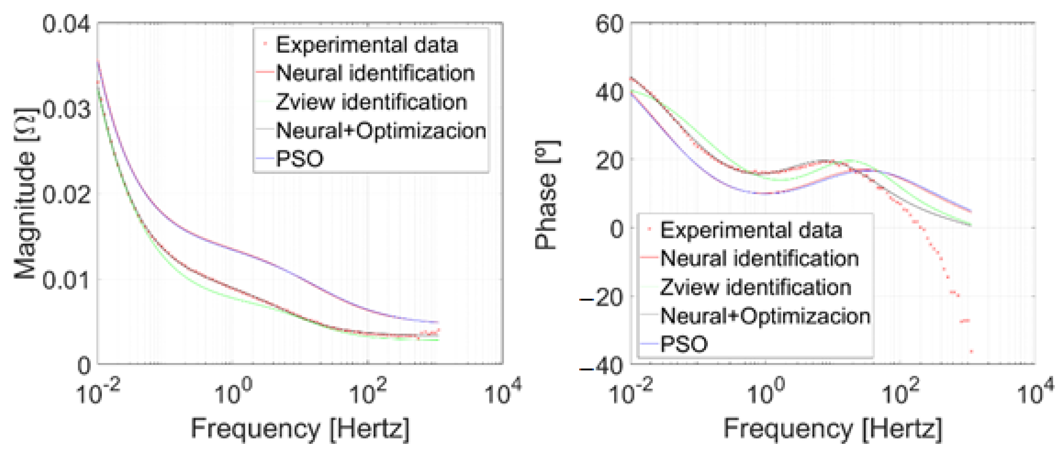
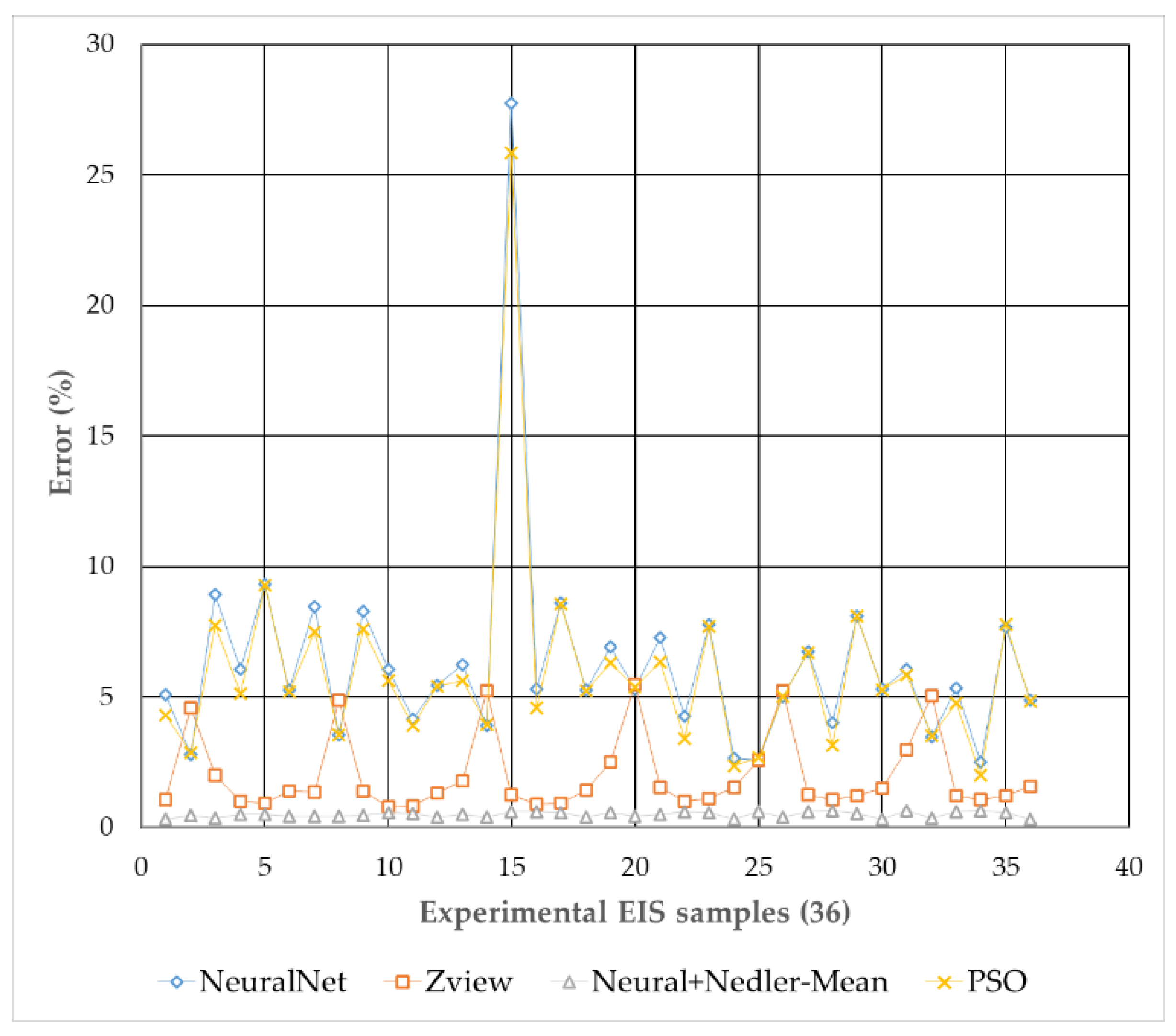
4.2. Algorithm’s Performance Comparison

The four algorithms of Section 3 have been tested with the 36 EIS experiments corresponding to 0%, 20%, 40%, 60%, 80%, and 100% of SOC at different-aged states during the six months of tests. The 36 EIS experiments come from the 6 different SOC values analyzed at 6 different experiment tests (1 per month). In all these experiments, authors compared the algorithm with the real experimental EIS results.
Figure 10 shows a sample set of experiments compared with the four algorithms as Nyquist plots. The equivalent circuit parameter values obtained with the proposed Neural + Optimization (black line) better match the desired real-time experimental data than those obtained with the other methods.
In Figure 11, the authors show the Bode diagram of a sample set of experiments with the four algorithms with Bode diagrams. The best results are achieved through combined identification between the artificial neural network and the Nelder–Mead algorithm. The high frequency behavior is not important for the authors’ objective because this inductive parameter does not give any information about State of Health.
The complete results corresponding to 36 experimental EIS datasets (that is included in the Supplementary Material) are somehow consistent with the ones reported in Figure 10. As it can be seen in Figure 12 the results corresponding to the hybrid neural network + Nelder–Mead Simplex method algorithm data series are the best for all 36 experiments.
Average error corresponding to the estimation of the EEC parameters of the four benchmarked methods for the 36 EIS experimental dataset is compared in Table 3.

5. Conclusions

The initial objective motivating this work sought to find a new and more accurate automatic identification procedure of EEC parameters from raw EIS data in order to implement monitoring variations of the earlier-mentioned EEC parameters.
The authors have benchmarked four different EEC parameter identification algorithms: Zview, neural network mapping EIS raw data to EEC parameters, Particle Swarm Optimization, and a new one using a neural network combined with the Nelder–Mead Simplex method.
We verified that the proposed augmentation data method used to train the neural network together with the Nelder–Mead simplex model has proven to be the best, performing, on average, 0.49% error for a given set of experimental EIS data and for a previously selected equivalent circuit. As compared to previous works of the authors where PSO was used with the same idea to initialize the Nelder–Mead, the authors believe that the neural networks offer lower computations cost for the final online implementation.
The method proposed in this work affords the advantage that offers a direct application of the suggested algorithm in subsequent monitoring of the equivalent circuit parameters’ evolution over the lifespan of the battery. Thus, the new hybrid model provides a valuable tool to automatically supervise the battery’s state of health at any time.
The complementary experimental data provided in the annexed file (Supplementary_Materials.zip) presents the results of the overall data sets corresponding to the six months of aging tests with a wide range of battery degradation and SOC conditions. Each experiment has been labelled where each corresponding plot is coded with the number of the month and the level of SOC. The 36 experiments correspond to six monthly data recording and six level of SOC per month, resulting in 36 battery conditions.

Supplementary Materials

The following supporting information can be downloaded at: https://www.mdpi.com/article/10.3390/batteries8110238/s1.

Author Contributions

Conceptualization, E.Z.; data curation, J.O. and J.G.-O.; formal analysis, J.M.d.I., E.Z. and J.M.L.-G.; funding acquisition, J.O.; investigation, J.O., J.M.d.I. and J.G.-O.; methodology, R.F.; project administration, R.F.; resources, J.O. and R.F.; software, J.M.d.I., E.Z. and J.G.-O.; supervision, E.Z. and J.M.L.-G.; validation, J.M.L.-G.; visualization, J.M.d.I.; writing—original draft, J.O.; writing—review and editing, J.M.L.-G. All authors have read and agreed to the published version of the manuscript.

Funding

Special thanks should also be expressed to the Torres Quevedo (PTQ) 2019 Aid from the State Research Agency, within the framework of the State Program for the Promotion of Talent and its Employability in R + D + i, Ref. PTQ2019-010787/AEI/10.13039/501100011033.

Acknowledgments

The authors express their gratitude to CIC energiGUNE for the facilities and to the Bcare innovation team for their technical and scientific contributions to this work.

Conflicts of Interest

The authors declare no conflict of interest.

References

  1. Bose, C.S.C.; Laman, F.C. Battery state of health estimation through coup de fouet. In Proceedings of the INTELEC. Twenty-Second International Telecommunications Energy Conference (Cat. No.00CH37131), Phoenix, AZ, USA, 10–14 September 2000; pp. 597–601. [Google Scholar] [CrossRef]
  2. Ng, K.-S.; Moo, C.-S.; Chen, Y.-P.; Hsieh, Y.-C. State-of-Charge Estimation for Lead-Acid Batteries Based on Dynamic Open-Circuit Voltage. In Proceedings of the 2008 IEEE 2nd International Power and Energy Conference, Johor Bahru, Malaysia, 1–3 December 2008; p. 5. [Google Scholar] [CrossRef]
  3. Li, A.; Pelissier, S.; Venet, P.; Gyan, P. Fast Characterization Method for Modeling Battery Relaxation Voltage. Batteries 2016, 2, 7. [Google Scholar] [CrossRef] [Green Version]
  4. Olarte, J.; de Ilarduya, J.M.; Zulueta, E.; Ferret, R.; Kurt, E.; Lopez-Guede, J.M. Estimating State of Charge and State of Health of Vented NiCd Batteries with Evolution of Electrochemical Parameters. JOM 2021, 73, 4085–4090. [Google Scholar] [CrossRef]
  5. Calborean, A.; Bruj, O.; Murariu, T.; Morari, C. Resonance frequency analysis of lead-acid cells: An EIS approach to predict the state-of-health. J. Energy Storage 2020, 27, 101143. [Google Scholar] [CrossRef]
  6. Badeda, J.; Kwiecien, M.; Schulte, D.; Sauer, D. Battery State Estimation for Lead-Acid Batteries under Float Charge Conditions by Impedance: Benchmark of Common Detection Methods. Appl. Sci. 2018, 8, 1308. [Google Scholar] [CrossRef] [Green Version]
  7. Pascoe, P.E.; Anbuky, A.H. Standby Power System VRLA Battery Reserve Life Estimation Scheme. IEEE Trans. Energy Convers. 2005, 20, 887–895. [Google Scholar] [CrossRef]
  8. Gopikanth, M.L.; Sathyanarayana, S. Impedance parameters and the state-of-charge. II. Lead-acid battery. J. Appl. Electrochem. 1979, 9, 369–379. [Google Scholar] [CrossRef]
  9. Huet, F. A review of impedance measurements for determination of the state-of-charge or state-of-health of secondary batteries. J. Power Sources 1998, 70, 59–69. [Google Scholar] [CrossRef]
  10. Lukács, Z.; Kristóf, T. A generalized model of the equivalent circuits in the electrochemical impedance spectroscopy. Electrochim. Acta 2020, 363, 137199. [Google Scholar] [CrossRef]
  11. Murariu, T.; Morari, C. Time-dependent analysis of the state-of-health for lead-acid batteries: An EIS study. J. Energy Storage 2019, 21, 87–93. [Google Scholar] [CrossRef]
  12. Harting, N.; Wolff, N.; Krewer, U. Identification of Lithium Plating in Lithium-Ion Batteries Using Nonlinear Frequency Response Analysis (NFRA). Electrochim. Acta 2018, 281, 378–385. [Google Scholar] [CrossRef]
  13. Kim, W.; Jang, D.; Kim, H.J. Understanding Electronic and Li-Ion Transport of LiNi0.5Co0.2Mn0.3O2 Electrodes Affected by Porosity and Electrolytes Using Electrochemical Impedance Spectroscopy. J. Power Sources 2021, 510, 230338. [Google Scholar] [CrossRef]
  14. Pastor-Fernández, C.; Uddin, K.; Chouchelamane, G.H.; Widanage, W.D.; Marco, J. A Comparison between Electrochemical Impedance Spectroscopy and Incremental Capacity-Differential Voltage as Li-Ion Diagnostic Techniques to Identify and Quantify the Effects of Degradation Modes within Battery Management Systems. J. Power Sources 2017, 360, 301–318. [Google Scholar] [CrossRef]
  15. Wang, X.; Wei, X.; Dai, H. Estimation of state of health of lithium-ion batteries based on charge transfer resistance considering different temperature and state of charge. J. Energy Storage 2019, 21, 618–631. [Google Scholar] [CrossRef]
  16. Olarte, J.; de Ilarduya, J.M.; Zulueta, E.; Ferret, R.; Fernández-Gámiz, U.; Lopez-Guede, J.M. A Battery Management System with EIS Monitoring of Life Expectancy for Lead–Acid Batteries. Electronics 2021, 10, 1228. [Google Scholar] [CrossRef]
  17. Lombardo, T.; Duquesnoy, M.; El-Bouysidy, H.; Årén, F.; Gallo-Bueno, A.; Jørgensen, P.B.; Bhowmik, A.; Demortière, A.; Ayerbe, E.; Alcaide, F.; et al. Artificial Intelligence Applied to Battery Research: Hype or Reality? Chem. Rev. 2022, 122, 10899–10960. [Google Scholar] [CrossRef]
  18. Kwiecien, M.; Badeda, J.; Huck, M.; Komut, K.; Duman, D.; Sauer, D. Determination of SoH of Lead-Acid Batteries by Electrochemical Impedance Spectroscopy. Appl. Sci. 2018, 8, 873. [Google Scholar] [CrossRef] [Green Version]
  19. Densmore, A.; Hanif, M. Determining Battery SoC Using Electrochemical Impedance Spectroscopy and the Extreme Learning Machine. In Proceedings of the 2015 IEEE 2nd International Future Energy Electronics Conference (IFEEC), Taipei, Taiwan, 1–4 November 2015. [Google Scholar]
  20. Kiel, M.; Sauer, D.U.; Turpin, P.; Naveed, M.; Favre, E. Validation of single frequency Z measurement for standby battery state of health determination. In Proceedings of the INTELEC 2008—2008 IEEE 30th International Telecommunications Energy Conference, San Diego, CA, USA, 14 September 2008; pp. 1–7. [Google Scholar] [CrossRef]
  21. Raijmakers, L.H.J.; Danilov, D.L.; van Lammeren, J.P.M.; Lammers, M.J.G.; Notten, P.H.L. Sensorless battery temperature measurements based on electrochemical impedance spectroscopy. J. Power Sources 2014, 247, 539–544. [Google Scholar] [CrossRef]
  22. Karden, E.; Buller, S.; de Doncker, R.W. A method for measurement and interpretation of impedance spectra for industrial batteries. J. Power Sources 2000, 85, 72–78. [Google Scholar] [CrossRef]
  23. Csomós, B.; Fodor, D. Identification of the material properties of an 18650 Li-ion battery for improving the electrochemical model used in cell testing. Hung. J. Ind. Chem. 2020, 48, 33–41. [Google Scholar] [CrossRef]
  24. Wang, X.; Wei, X.; Zhu, J.; Dai, H.; Zheng, Y.; Xu, X.; Chen, Q. A review of modeling, acquisition, and application of lithium-ion battery impedance for onboard battery management. eTransportation 2021, 7, 100093. [Google Scholar] [CrossRef]
  25. Chun, H.; Kim, J.; Han, S. Parameter identification of an electrochemical lithium-ion battery model with convolutional neural network. IFAC-PapersOnLine 2019, 52, 129–134. [Google Scholar] [CrossRef]
  26. Jiménez-Bermejo, D.; Fraile-Ardanuy, J.; Castaño-Solis, S.; Merino, J.; Álvaro-Hermana, R. Using Dynamic Neural Networks for Battery State of Charge Estimation in Electric Vehicles. Procedia Comput. Sci. 2018, 130, 533–540. [Google Scholar] [CrossRef]
  27. Yang, D.; Wang, Y.; Pan, R.; Chen, R.; Chen, Z. A Neural Network Based State-of-Health Estimation of Lithium-ion Battery in Electric Vehicles. Energy Procedia 2017, 105, 2059–2064. [Google Scholar] [CrossRef]
  28. Capizzi, G.; Bonanno, F.; Tina, G.M. Recurrent Neural Network-Based Modeling and Simulation of Lead-Acid Batteries Charge-Discharge. IEEE Trans. Energy Convers. 2011, 26, 435–443. [Google Scholar] [CrossRef]
  29. Young, R.E.; Li, X.; Perone, S.P. Prediction of individual cell performance in a long-string lead/acid peak-shaving battery: Application of artificial neural networks. J. Power Sources 1996, 62, 121–134. [Google Scholar] [CrossRef]
  30. Morita, Y.; Yamamoto, S.; Lee, S.H.; Mizuno, N. On-line detection of state-of-charge in lead acid battery using both neural network and on-line identification. In Proceedings of the Iecon 2006—32nd Annual Conference on IEEE Industrial Electronics, Paris, France, 6–10 November 2006; Volume 1–11, pp. 3379–3384. [Google Scholar]
  31. Lagarias, J.C.; Reeds, J.A.; Wright, M.H.; Wright, P.E. Convergence Properties of the Nelder—Mead Simplex Method in Low Dimensions. SIAM J. Optim. 1998, 9, 112–147. [Google Scholar] [CrossRef] [Green Version]
  32. Olarte, J.; de Ilarduya, J.M.; Zulueta, E.; Ferret, R.; Fernández-Gámiz, U.; Lopez-Guede, J.M. Automatic Identification Algorithm of Equivalent Electrochemical Circuit Based on Electroscopic Impedance Data for a Lead Acid Battery. Electronics 2021, 10, 1353. [Google Scholar] [CrossRef]
  33. Komsiyska, L.; Buchberger, T.; Diehl, S.; Ehrensberger, M.; Hanzl, C.; Hartmann, C.; Hölzle, M.; Kleiner, J.; Lewerenz, M.; Liebhart, B.; et al. Critical Review of Intelligent Battery Systems: Challenges, Implementation, and Potential for Electric Vehicles. Energies 2021, 14, 5989. [Google Scholar] [CrossRef]
  34. Hornik, K. Approximation capabilities of multilayer feedforward networks. Neural Netw. 1991, 4, 251–257. [Google Scholar] [CrossRef]
Figure 1. Sample Nyquist plots for a new and aged battery at different temperatures and SOC.
Batteries 08 00238 g001
Figure 2. (a) Equivalent proposed EEC circuit model and (b) Adjustment of the EIS of the 12 V block at the 100% state of charge (SOC) using Zview software.
Batteries 08 00238 g002
Figure 3. Data augmentation detailed flowchart.
Batteries 08 00238 g003
Figure 4. Flow-chart processes for (a) data augmentation and (b) best NN selection to map EIS to the Nelder–Mead Initialization values.
Batteries 08 00238 g004
Figure 5. Example of the accepted electrochemical impedance spectra generated by augmented data.
Batteries 08 00238 g005
Figure 6. Error Histogram 10 neurons after 100 epochs.
Batteries 08 00238 g006
Figure 7. Error histogram with 10 neurons and 200 epochs.
Batteries 08 00238 g007
Figure 8. Error histogram with 5 neurons and 100 epochs.
Batteries 08 00238 g008
Figure 9. Error histogram with 20 neurons and 100 epochs.
Batteries 08 00238 g009
Figure 10. Final results and comparison with the experimental data.
Batteries 08 00238 g010
Figure 11. Bode diagrams of final results and comparison with the experimental data.
Batteries 08 00238 g011
Figure 12. Final results and comparison with the experimental data.
Batteries 08 00238 g012
Table 1. Parameters extracted from the EIS using manual adjustments in the Zview software.
SoHR1CPE1-TCPE1-PR2CPE2-TCPE2-PR3
100%0.00271767.170.857290.009217487.180.65421-
80%0.00279539.210.778650.0039696184.130.612210.21606
60%0.003134911.210.759090.0021683218.800.568470.08871
40%0.003345218.010.620910.0020905229.500.500600.066692
20%0.003958414.920.657450.0020599199.400.381220.12304
0%0.004677510.120.708040.0025044152.200.29418-
Table 2. Neural network analysis with different conditions. MSE loss function is calculated with the test dataset.
NeuronsEpochsMin ErrorMax ErrorGradientMSE Loss Function
10100−0.000210.0009041.4505 × 10−41.2121 × 10⁻⁶
10200−0.00030.0003835.8395 × 10−43.3363 × 10⁻⁷
5100−0.001220.0010069.2107 × 10−61.9786 × 10⁻⁶
20100−0.000760.0001773.7085 × 10−48.3897 × 10⁻⁷
Table 3. Average error of the four benchmarked methods for the 36 EIS experimental dataset.
Benchmarked MethodAverage Error
MeanErrorNeural6.29%
MeanErrorZview2.01%
MeanErrorNeuralOpt0.49%
MeanErrorPso5.92%
Publisher’s Note: MDPI stays neutral with regard to jurisdictional claims in published maps and institutional affiliations.

