
Physics-Based SoH Estimation for Li-Ion Cells

Abstract
:1. Introduction
- Defining a suitable EIS-based SoH estimation model which uses degradation indicators directly linked to DMs, allowing principled modelling of the physical phenomena (i.e., physics-based SoH estimation);
- Defining a simple and robust framework that could be exploited for online-SoH estimation by next generation smart BMSs based on (i) an appropriate testing campaign to initialize the SoH estimation model for a new Li-ion chemistry/model and (ii) the capability to run onboard EIS measurement.
2. Materials and Methods
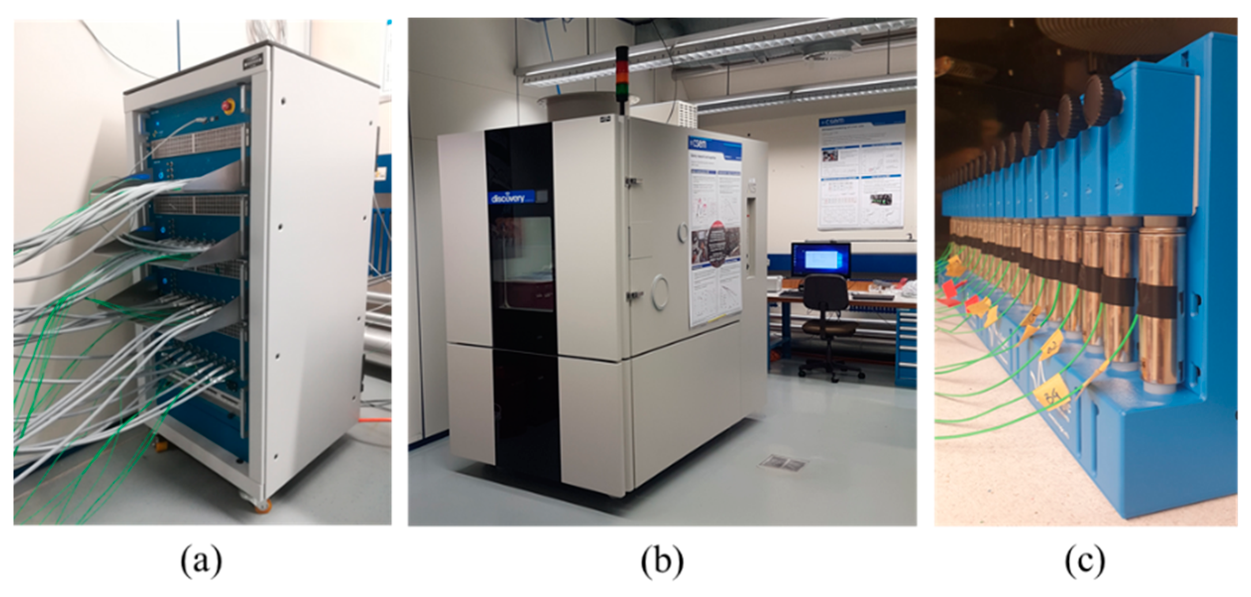
2.1. Inputs: Experimental Dataset and DRT Characterization
2.2. Methodology
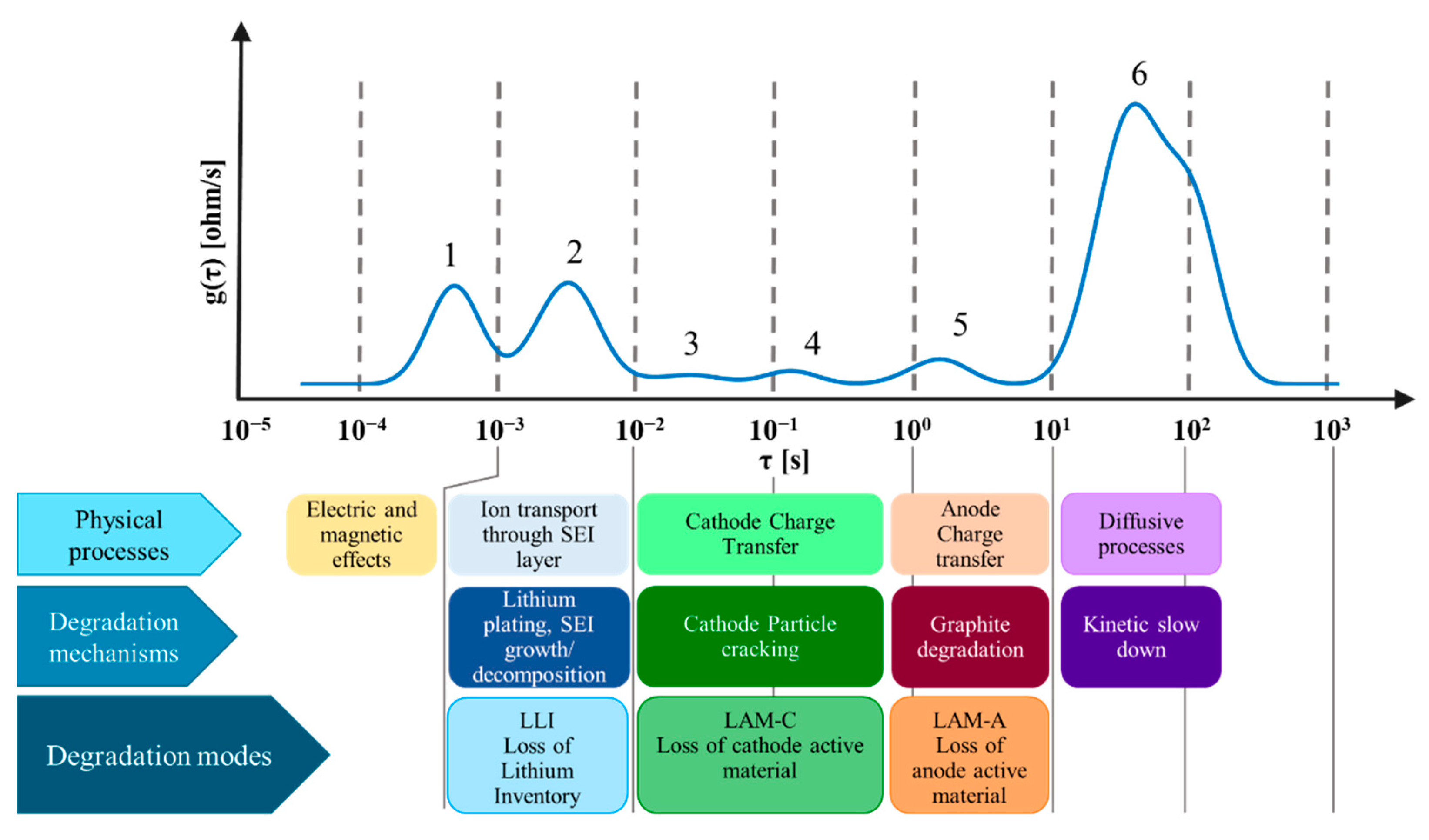
- Peak 2 is attributed to the growth and decomposition of SEI layer and presence of lithium plating on the anode side; it will be used to account for Loss of Lithium Inventory ();
- Peak 3 and peak 4 are attributed to cathode degradation (specifically particle cracking for NMC811) and they are therefore used to account for Loss of Cathode Active Material ();
- Peak 5 is attributed to graphite degradation and it is hence used to account for Loss of Anode Active Material ().
2.2.1. Degradation Indicators
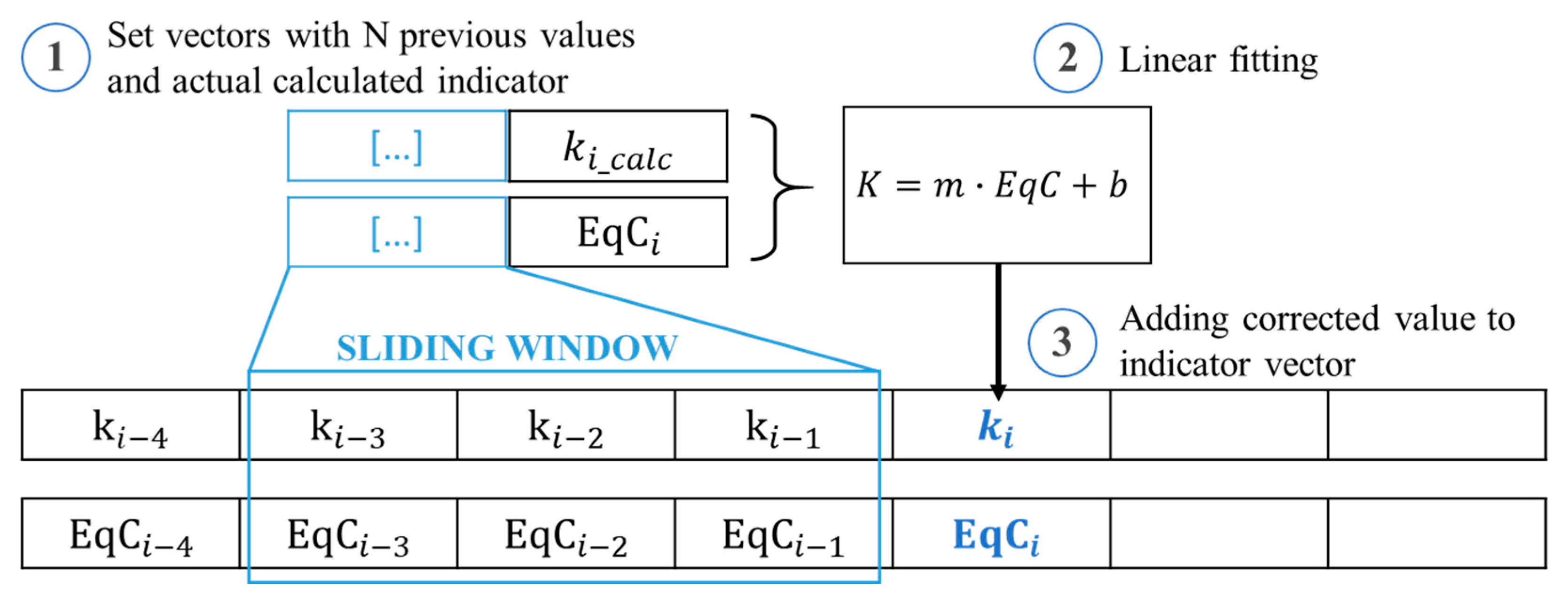
- A set of prior points is selected based on a sliding window of size W and is concatenated with the indicator computed at diagnosis step ;
- A linear fitting model is applied to the selected vectors;
- The linear model is used to compute the corrected value of
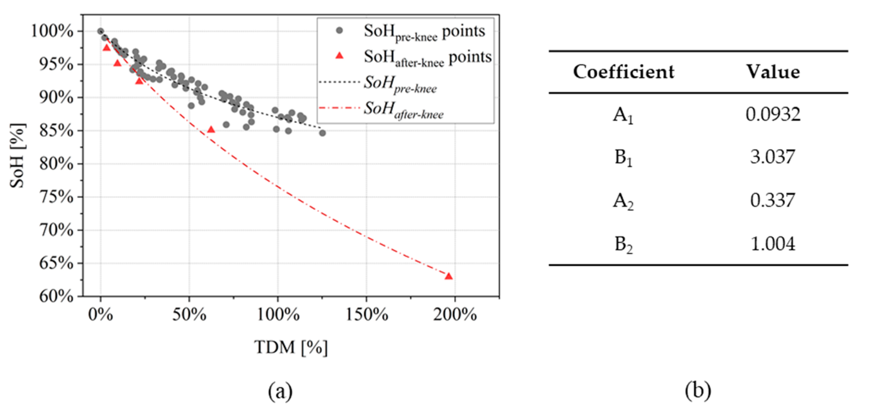
2.2.2. SoH Estimation
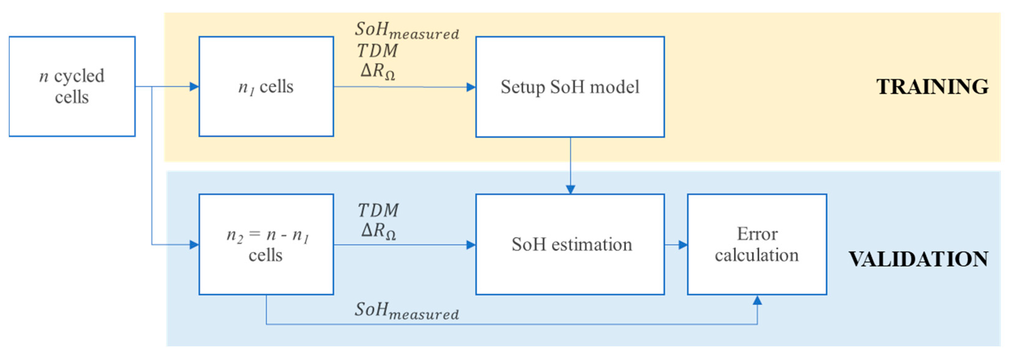
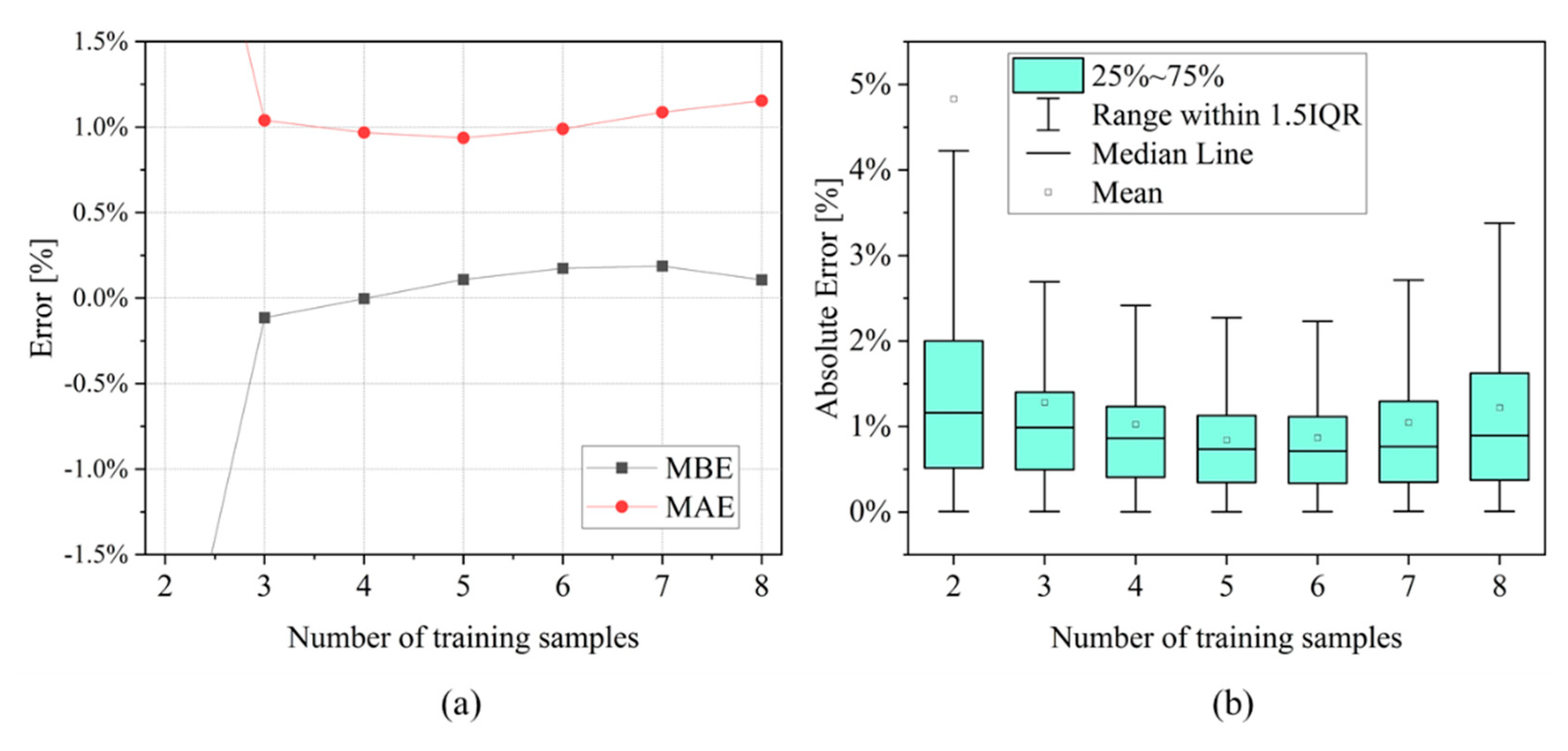
- Training subset: n1 cells are selected and their EIS measurements are used to compute degradation indicators and ohmic indicator. SoH values are fitted to find the parameters of the model described in Equation (6).
- Validation subset: n2 cells (i.e., n2 = 10 − n1) are used to compute the indicator and the SoH is estimated with the SoH model checking the value of . Finally, the estimated value is compared with the one computed by capacity measurement.
3. Results
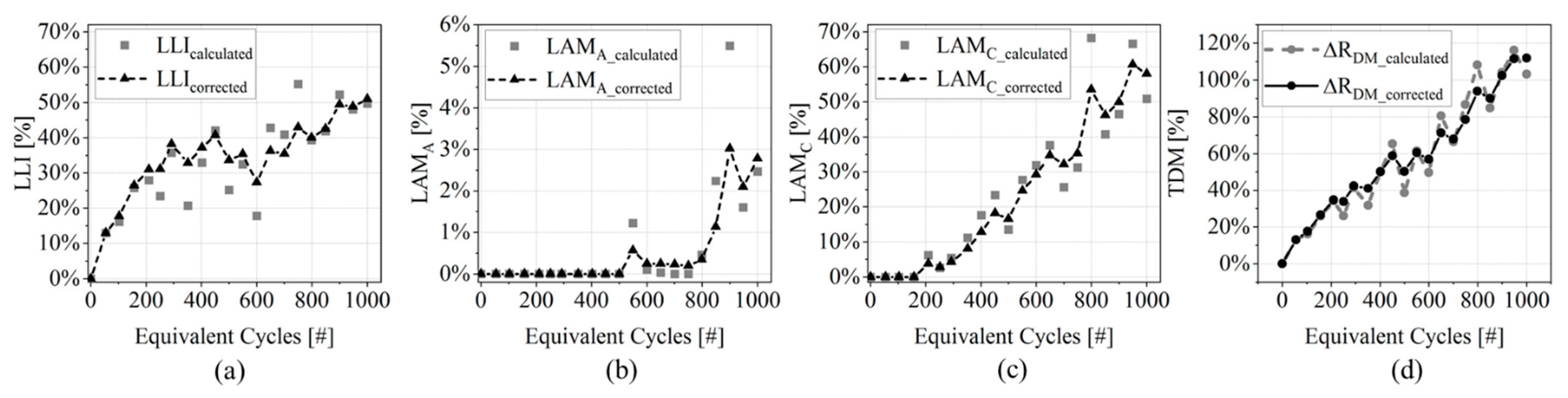
3.1. Degradation Indicators
- (Figure 7a): a monotonic growth is observed until around 400 EqC when the indicator decreases its growth and starts to oscillate;
- (Figure 7c): cell’s cathode is not impacted by degradation until 200 EqC; after this point it shows a constant growth up to 60% at 1000 EqC;
- (Figure 7b): this DM is not affecting cell performances until about 800 EqC. Moreover, its magnitude is one order of magnitude lower than the other two indicators.
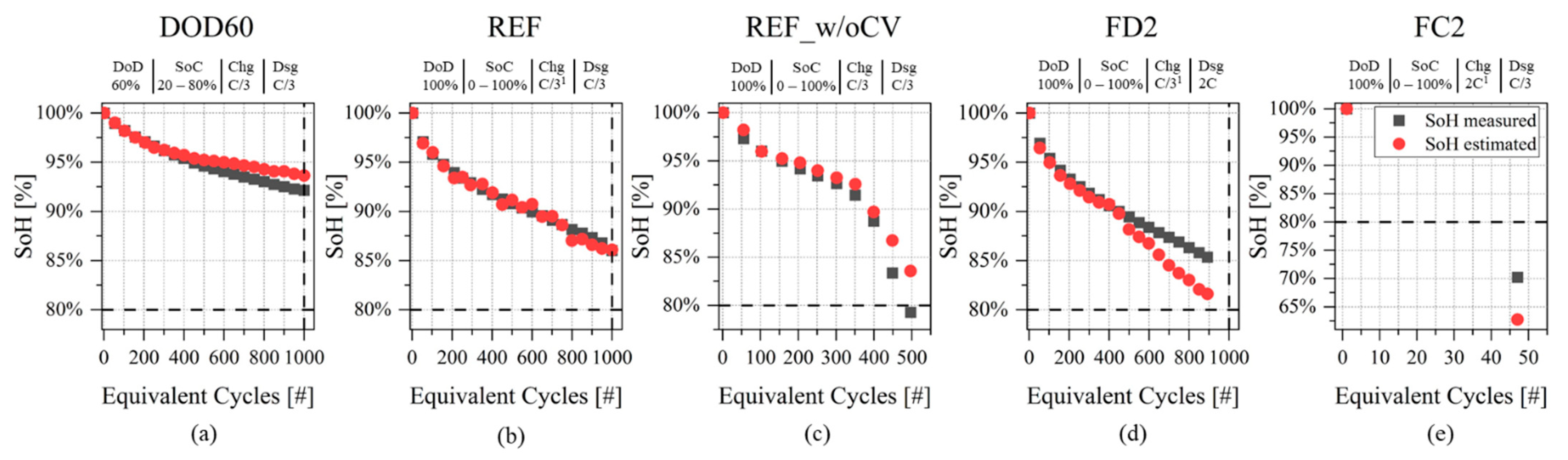
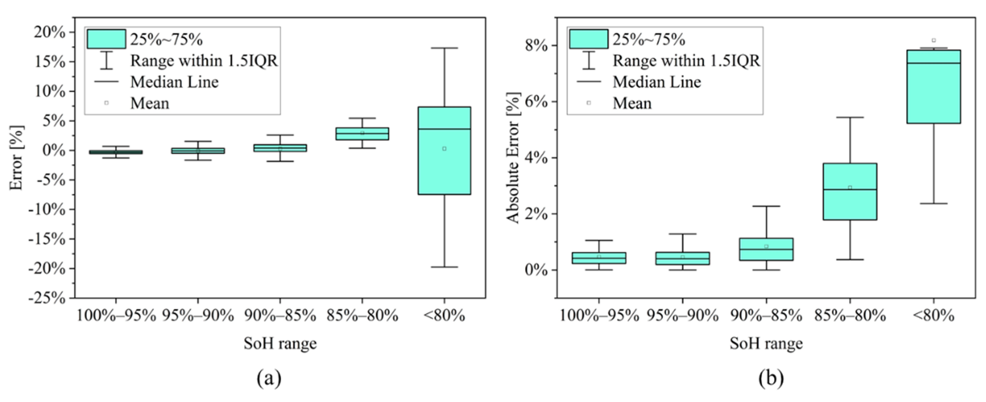
3.2. SoH Estimation
4. Discussion
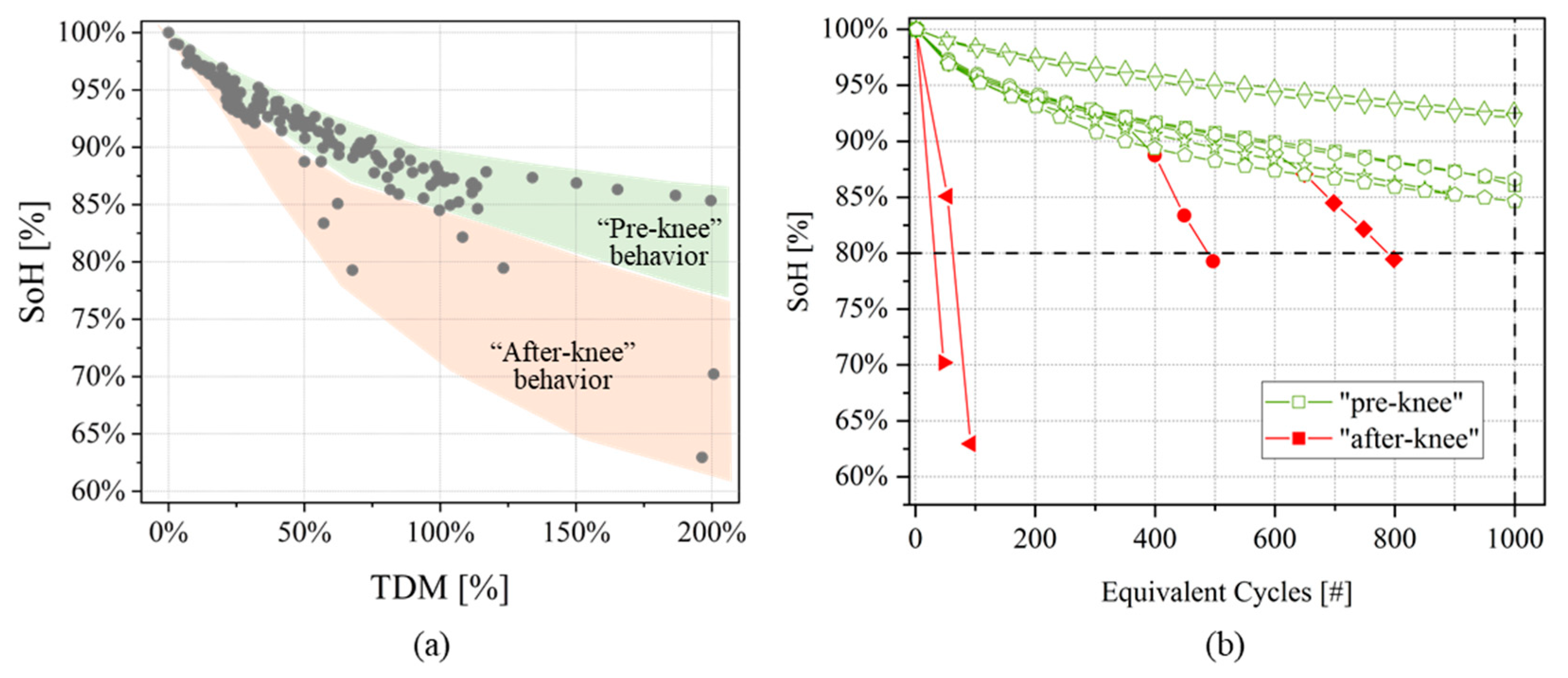
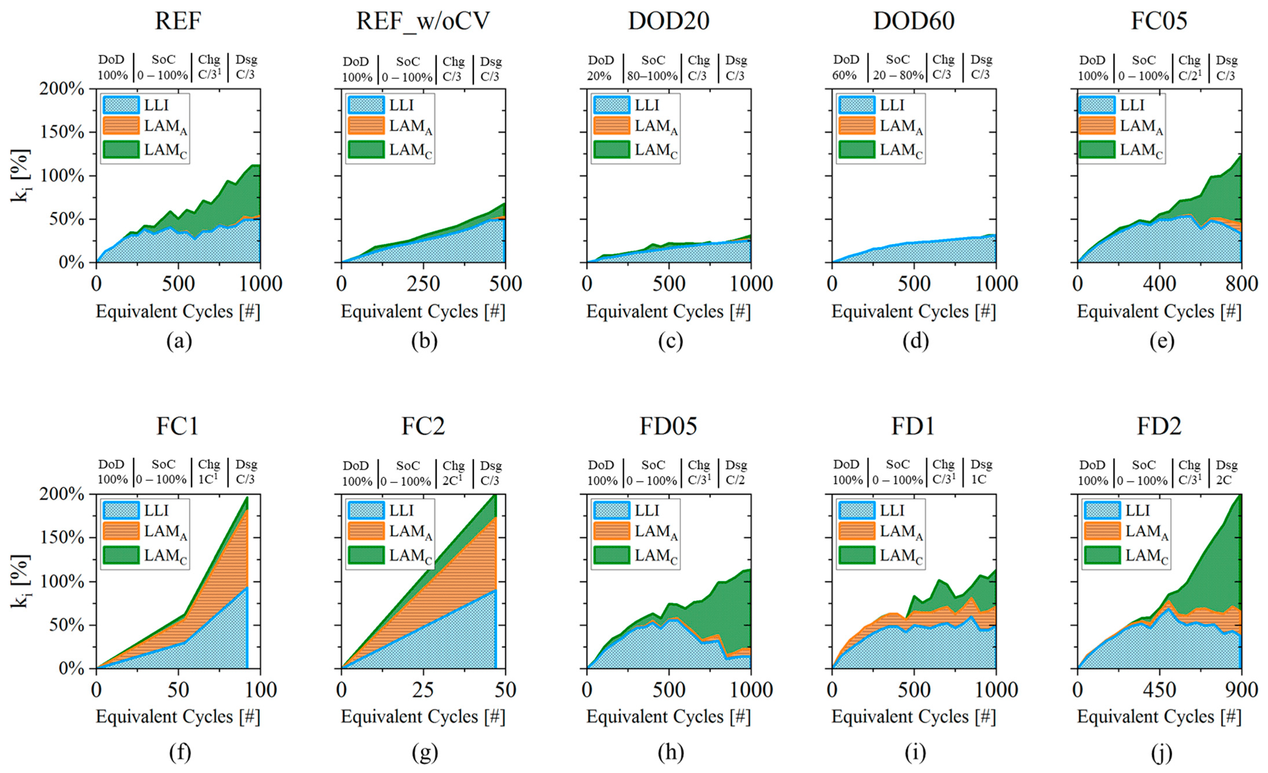
- Plan relevant aging tests that cover different aging behaviors and allow to train the SoH model both for “pre-knee” and “after-knee” conditions. The selected protocols should include: (i) reduced DoD condition to appreciate slow degradation (i.e., capacity fade); (ii) nominal conditions, to verify the specifications from the manufacturer; (iii) moderate charging or discharging conditions that accelerates degradation with respect to nominal conditions and that could guarantee both “pre-knee” and “after-knee behavior” (such as cell ID:FC05) and (iv) high charging or discharging rate that guarantee fast degradation and “after-knee” conditions (such as cell ID:FC2);
- Perform diagnosis phase (capacity + EIS measurements) at a fixed number of EqC down to a certain value of SoH (e.g., 85%) and then intensify the number of checks by lowering the number of cycles in each repetition. In this way, more measurements will be available in the region where is mainly occurring the “knee” and accelerated capacity fade, reducing the SoH estimation error;
- Run sensitivity analysis on the ohmic resistance variation parameter to discriminate between “pre-knee” and “after-knee” conditions with a suitable threshold. Validation can be performed graphically on SoH evolution curves as done in Figure 5.
- Run “diagnosis” based on long-EIS measurements (10 kHz–10 mHz). Select an appropriate criterion on when to acquire two consecutives full-EIS measurements. Depending on battery application, this variable could be set based on cycles number, a fixed period of time, or randomly (e.g., exploiting resting periods during application);
- Run “check-up” based on short-EIS measurements only at high frequency (10 kHz–1 kHz) to frequently update , which is crucial to activate additional “diagnosis” measurements whenever the “after-knee” behavior is reached based on the computation (Section 2.2.2). Additional “diagnosis” can also be activated under a certain estimated value of SoH (e.g., 85%);
- Compute the degradation indicators whenever possible to understand if unexpected behaviors are happening inside the cell. This can be done by updating DMs values and by analyzing them over time and/or over cycle number.
5. Conclusions
Author Contributions
Funding
Data Availability Statement
Conflicts of Interest
References
- Armand, M.; Tarascon, J.-M. Building Better Batteries. Nature 2008, 451, 652–657. [Google Scholar] [CrossRef] [PubMed]
- Bresser, D.; Moretti, A.; Varzi, A.; Passerini, S. The Role of Batteries for the Successful Transition to Renewable Energy Sources. In Encyclopedia of Electrochemistry; John Wiley & Sons, Ltd.: New York, NY, USA, 2020; pp. 1–9. ISBN 978-3-527-61042-6. [Google Scholar]
- Armand, M.; Axmann, P.; Bresser, D.; Copley, M.; Edström, K.; Ekberg, C.; Guyomard, D.; Lestriez, B.; Novák, P.; Petranikova, M.; et al. Lithium-Ion Batteries—Current State of the Art and Anticipated Developments. J. Power Source 2020, 479, 228708. [Google Scholar] [CrossRef]
- Berckmans, G.; Messagie, M.; Smekens, J.; Omar, N.; Vanhaverbeke, L.; Van Mierlo, J. Cost Projection of State of the Art Lithium-Ion Batteries for Electric Vehicles Up to 2030. Energies 2017, 10, 1314. [Google Scholar] [CrossRef] [Green Version]
- Marinaro, M.; Bresser, D.; Beyer, E.; Faguy, P.; Hosoi, K.; Li, H.; Sakovica, J.; Amine, K.; Wohlfahrt-Mehrens, M.; Passerini, S. Bringing Forward the Development of Battery Cells for Automotive Applications: Perspective of R&D Activities in China, Japan, the EU and the USA. J. Power Source 2020, 459, 228073. [Google Scholar] [CrossRef]
- Tsujikawa, T.; Yabuta, K.; Arakawa, M.; Hayashi, K. Safety of Large-Capacity Lithium-Ion Battery and Evaluation of Battery System for Telecommunications. J. Power Source 2013, 244, 11–16. [Google Scholar] [CrossRef]
- Hu, Y.; Yurkovich, S.; Guezennec, Y.; Yurkovich, B.J. Electro-Thermal Battery Model Identification for Automotive Applications. J. Power Source 2011, 196, 449–457. [Google Scholar] [CrossRef]
- Rahimi-Eichi, H.; Ojha, U.; Baronti, F.; Chow, M.-Y. Battery Management System: An Overview of Its Application in the Smart Grid and Electric Vehicles. IEEE Ind. Electron. Mag. 2013, 7, 4–16. [Google Scholar] [CrossRef]
- Birkl, C.R.; Roberts, M.R.; McTurk, E.; Bruce, P.G.; Howey, D.A. Degradation Diagnostics for Lithium Ion Cells. J. Power Source 2017, 341, 373–386. [Google Scholar] [CrossRef]
- Barré, A.; Deguilhem, B.; Grolleau, S.; Gérard, M.; Suard, F.; Riu, D. A Review on Lithium-Ion Battery Ageing Mechanisms and Estimations for Automotive Applications. J. Power Source 2013, 241, 680–689. [Google Scholar] [CrossRef] [Green Version]
- Dubarry, M.; Truchot, C.; Liaw, B.Y. Synthesize Battery Degradation Modes via a Diagnostic and Prognostic Model. J. Power Source 2012, 219, 204–216. [Google Scholar] [CrossRef]
- Pop, V.; Bergveld, H.J.; Regtien, P.P.L.; Veld, J.H.G.O.H.; Danilov, D.; Notten, P.H.L. Battery Aging and Its Influence on the Electromotive Force. J. Electrochem. Soc. 2007, 154, A744. [Google Scholar] [CrossRef]
- Waag, W.; Fleischer, C.; Sauer, D. Critical Review of the Methods for Monitoring of Lithium-Ion Batteries in Electric and Hybrid Vehicles. J. Power Source 2014, 258, 321–339. [Google Scholar] [CrossRef]
- Brivio, C.; Carrillo, R.E.; Alet, P.-J.; Hutter, A. BestimatorTM: A Novel Model-Based Algorithm for Robust Estimation of Battery SoC. In Proceedings of the 2020 International Symposium on Power Electronics, Electrical Drives, Automation and Motion (SPEEDAM), Sorrento, Italy, 24–26 June 2020; pp. 184–188. [Google Scholar]
- Dai, H.; Jiang, B.; Hu, X.; Lin, X.; Wei, X.; Pecht, M. Advanced Battery Management Strategies for a Sustainable Energy Future: Multilayer Design Concepts and Research Trends. Renew. Sustain. Energy Rev. 2021, 138, 110480. [Google Scholar] [CrossRef]
- Pastor-Fernández, C.; Yu, T.F.; Widanage, W.D.; Marco, J. Critical Review of Non-Invasive Diagnosis Techniques for Quantification of Degradation Modes in Lithium-Ion Batteries. Renew. Sustain. Energy Rev. 2019, 109, 138–159. [Google Scholar] [CrossRef]
- Zhang, Q.; Wang, D.; Schaltz, E.; Stroe, D.-I.; Gismero, A.; Yang, B. Degradation Mechanism Analysis and State-of-Health Estimation for Lithium-Ion Batteries Based on Distribution of Relaxation Times. J. Energy Storage 2022, 55, 105386. [Google Scholar] [CrossRef]
- Marongiu, A.; Nlandi, N.; Rong, Y.; Sauer, D.U. On-Board Capacity Estimation of Lithium Iron Phosphate Batteries by Means of Half-Cell Curves. J. Power Source 2016, 324, 158–169. [Google Scholar] [CrossRef]
- Pastor-Fernández, C.; Uddin, K.; Chouchelamane, G.H.; Widanage, W.D.; Marco, J. A Comparison between Electrochemical Impedance Spectroscopy and Incremental Capacity-Differential Voltage as Li-Ion Diagnostic Techniques to Identify and Quantify the Effects of Degradation Modes within Battery Management Systems. J. Power Source 2017, 360, 301–318. [Google Scholar] [CrossRef]
- Anseán, D.; Baure, G.; González, M.; Cameán, I.; García, A.B.; Dubarry, M. Mechanistic Investigation of Silicon-Graphite/LiNi0.8Mn0.1Co0.1O2 Commercial Cells for Non-Intrusive Diagnosis and Prognosis. J. Power Source 2020, 459, 227882. [Google Scholar] [CrossRef]
- Schaltz, E.; Stroe, D.-I.; Nørregaard, K.; Ingvardsen, L.S.; Christensen, A. Incremental Capacity Analysis Applied on Electric Vehicles for Battery State-of-Health Estimation. IEEE Trans. Ind. Appl. 2021, 57, 1810–1817. [Google Scholar] [CrossRef]
- Lin, C.P.; Cabrera, J.; Yu, D.Y.W.; Yang, F.; Tsui, K.L. SOH Estimation and SOC Recalibration of Lithium-Ion Battery with Incremental Capacity Analysis & Cubic Smoothing Spline. J. Electrochem. Soc. 2020, 167, 090537. [Google Scholar] [CrossRef]
- Brivio, C.; Musolino, V.; Merlo, M.; Ballif, C. A Physically-Based Electrical Model for Lithium-Ion Cells. IEEE Trans. Energy Convers. 2019, 34, 594–603. [Google Scholar] [CrossRef]
- Illig, J.; Schmidt, J.P.; Weiss, M.; Weber, A.; Ivers-Tiffée, E. Understanding the Impedance Spectrum of 18650 LiFePO4-Cells. J. Power Source 2013, 239, 670–679. [Google Scholar] [CrossRef]
- Meddings, N.; Heinrich, M.; Overney, F.; Lee, J.-S.; Ruiz, V.; Napolitano, E.; Seitz, S.; Hinds, G.; Raccichini, R.; Gaberšček, M.; et al. Application of Electrochemical Impedance Spectroscopy to Commercial Li-Ion Cells: A Review. J. Power Source 2020, 480, 228742. [Google Scholar] [CrossRef]
- Iurilli, P.; Brivio, C.; Wood, V. On the Use of Electrochemical Impedance Spectroscopy to Characterize and Model the Aging Phenomena of Lithium-Ion Batteries: A Critical Review. J. Power Source 2021, 505, 229860. [Google Scholar] [CrossRef]
- Boukamp, B.A. Distribution (Function) of Relaxation Times, Successor to Complex Nonlinear Least Squares Analysis of Electrochemical Impedance Spectroscopy? J. Phys. Energy 2020, 2, 042001. [Google Scholar] [CrossRef]
- Bartoszek, J.; Liu, Y.-X.; Karczewski, J.; Wang, S.-F.; Mrozinski, A.; Jasinski, P. Distribution of Relaxation Times as a Method of Separation and Identification of Complex Processes Measured by Impedance Spectroscopy. In Proceedings of the 2017 21st European Microelectronics and Packaging Conference (EMPC) & Exhibition, Warsaw, Poland, 10–13 September 2017; pp. 1–5. [Google Scholar]
- Schichlein, H.; Ller, A.C.M.; Voigts, M. Deconvolution of Electrochemical Impedance Spectra for the Identification of Electrode Reaction Mechanisms in Solid Oxide Fuel Cells. J. Appl. Electrochem. 2002, 32, 875–882. [Google Scholar] [CrossRef]
- Zhou, X.; Pan, Z.; Han, X.; Lu, L.; Ouyang, M. An Easy-to-Implement Multi-Point Impedance Technique for Monitoring Aging of Lithium Ion Batteries. J. Power Source 2019, 417, 188–192. [Google Scholar] [CrossRef]
- Zhou, X.; Huang, J.; Pan, Z.; Ouyang, M. Impedance Characterization of Lithium-Ion Batteries Aging under High-Temperature Cycling: Importance of Electrolyte-Phase Diffusion. J. Power Source 2019, 426, 216–222. [Google Scholar] [CrossRef]
- Carthy, K.M.; Gullapalli, H.; Ryan, K.M.; Kennedy, T. Review—Use of Impedance Spectroscopy for the Estimation of Li-Ion Battery State of Charge, State of Health and Internal Temperature. J. Electrochem. Soc. 2021, 168, 080517. [Google Scholar] [CrossRef]
- Jiang, S.; Song, Z. Estimating the State of Health of Lithium-Ion Batteries with a High Discharge Rate through Impedance. Energies 2021, 14, 4833. [Google Scholar] [CrossRef]
- Mingant, R.; Bernard, J.; Sauvant Moynot, V.; Delaille, A.; Mailley, S.; Hognon, J.-L.; Huet, F. EIS Measurements for Determining the SoC and SoH of Li-Ion Batteries. ECS Trans. 2019, 33, 41–53. [Google Scholar] [CrossRef]
- Galeotti, M.; Cinà, L.; Giammanco, C.; Cordiner, S.; Di Carlo, A. Performance Analysis and SOH (State of Health) Evaluation of Lithium Polymer Batteries through Electrochemical Impedance Spectroscopy. Energy 2015, 89, 678–686. [Google Scholar] [CrossRef]
- Chen, L.; Lü, Z.; Lin, W.; Li, J.; Pan, H. A New State-of-Health Estimation Method for Lithium-Ion Batteries through the Intrinsic Relationship between Ohmic Internal Resistance and Capacity. Measurement 2018, 116, 586–595. [Google Scholar] [CrossRef]
- Dam, S.K.; John, V. High-Resolution Converter for Battery Impedance Spectroscopy. IEEE Trans. Ind. Appl. 2018, 54, 1502–1512. [Google Scholar] [CrossRef]
- Wang, X.; Wei, X.; Chen, Q.; Dai, H. A Novel System for Measuring Alternating Current Impedance Spectra of Series-Connected Lithium-Ion Batteries With a High-Power Dual Active Bridge Converter and Distributed Sampling Units. IEEE Trans. Ind. Electron. 2021, 68, 7380–7390. [Google Scholar] [CrossRef]
- Hoshi, Y.; Yakabe, N.; Isobe, K.; Saito, T.; Shitanda, I.; Itagaki, M. Wavelet Transformation to Determine Impedance Spectra of Lithium-Ion Rechargeable Battery. J. Power Source 2016, 315, 351–358. [Google Scholar] [CrossRef]
- Namor, E.; Brivio, C.; Le Roux, E. Battery System and Battery Management Method. European Patent WO 2022/200476 A1, 29 September 2022. [Google Scholar]
- Infineon Technologies Evaluation Board—Infineon Technologies. Available online: https://www.infineon.com/cms/en/design-support/finder-selection-tools/product-finder/evaluation-board/ (accessed on 22 September 2022).
- Infineon Technologies TLE9012DQU|Li-Ion Battery Monitoring and Balancing IC—Infineon Technologies. Available online: https://www.infineon.com/cms/en/product/battery-management-ics/tle9012dqu/ (accessed on 22 September 2022).
- Iurilli, P.; Brivio, C.; Carrillo, R.E.; Wood, V. EIS2MOD: A DRT-Based Modeling Framework for Li-Ion Cells. IEEE Trans. Ind. Appl. 2022, 58, 1429–1439. [Google Scholar] [CrossRef]
- Iurilli, P.; Brivio, C.; Wood, V. Detection of Lithium-Ion Cells’ Degradation through Deconvolution of Electrochemical Impedance Spectroscopy with Distribution of Relaxation Time. Energy Technol. 2022, 10, 2200547. [Google Scholar] [CrossRef]
- Product Specifications—Battery Tester BCS-800 Series. Available online: https://www.biologic.net/documents/hight-throughput-battery-tester-bcs-8xx-series/ (accessed on 16 April 2021).
- Angelantoni Test Technologies Discovery Climatic Chambers. Available online: https://www.acstestchambers.com/en/environmental-test-chambers/discovery-my-climatic-chambers-for-stress-screening/ (accessed on 16 April 2021).
- Attia, P.M.; Bills, A.; Planella, F.B.; Dechent, P.; dos Reis, G.; Dubarry, M.; Gasper, P.; Gilchrist, R.; Greenbank, S.; Howey, D.; et al. Review—“Knees” in Lithium-Ion Battery Aging Trajectories. J. Electrochem. Soc. 2022, 169, 060517. [Google Scholar] [CrossRef]
- Schuster, S.F.; Bach, T.; Fleder, E.; Müller, J.; Brand, M.; Sextl, G.; Jossen, A. Nonlinear Aging Characteristics of Lithium-Ion Cells under Different Operational Conditions. J. Energy Storage 2015, 1, 44–53. [Google Scholar] [CrossRef]
- Diao, W.; Saxena, S.; Han, B.; Pecht, M. Algorithm to Determine the Knee Point on Capacity Fade Curves of Lithium-Ion Cells. Energies 2019, 12, 2910. [Google Scholar] [CrossRef] [Green Version]
- Boukamp, B.A. A Linear Kronig-Kramers Transform Test for Immittance Data Validation. J. Electrochem. Soc. 1995, 142, 1885. [Google Scholar] [CrossRef]
- Hahn, M.; Schindler, S.; Triebs, L.-C.; Danzer, M.A. Optimized Process Parameters for a Reproducible Distribution of Relaxation Times Analysis of Electrochemical Systems. Batteries 2019, 5, 43. [Google Scholar] [CrossRef] [Green Version]
- Wan, T.H.; Saccoccio, M.; Chen, C.; Ciucci, F. Influence of the Discretization Methods on the Distribution of Relaxation Times Deconvolution: Implementing Radial Basis Functions with DRTtools. Electrochim. Acta 2015, 184, 483–499. [Google Scholar] [CrossRef]
- Gavrilyuk, A.L.; Osinkin, D.A.; Bronin, D.I. The Use of Tikhonov Regularization Method for Calculating the Distribution Function of Relaxation Times in Impedance Spectroscopy. Russ. J. Electrochem. 2017, 53, 575–588. [Google Scholar] [CrossRef]
- Wildfeuer, L.; Wassiliadis, N.; Karger, A.; Bauer, F.; Lienkamp, M. Teardown Analysis and Characterization of a Commercial Lithium-Ion Battery for Advanced Algorithms in Battery Electric Vehicles. J. Energy Storage 2022, 48, 103909. [Google Scholar] [CrossRef]
- Yang, X.-G.; Leng, Y.; Zhang, G.; Ge, S.; Wang, C.-Y. Modeling of Lithium Plating Induced Aging of Lithium-Ion Batteries: Transition from Linear to Nonlinear Aging. J. Power Source 2017, 360, 28–40. [Google Scholar] [CrossRef]
- Capron, O.; Gopalakrishnan, R.; Jaguemont, J.; Van den Bossche, P.; Omar, N.; Van Mierlo, J. On the Ageing of High Energy Lithium-Ion Batteries—Comprehensive Electrochemical Diffusivity Studies of Harvested Nickel Manganese Cobalt Electrodes. Materials 2018, 11, 176. [Google Scholar] [CrossRef]
- Yi, M.; Jiang, F.; Zhao, G.; Guo, D.; Ren, D.; Lu, L.; Ouyang, M. Detection of Lithium Plating Based on the Distribution of Relaxation Times. In Proceedings of the 2021 IEEE 4th International Electrical and Energy Conference (CIEEC), Wuhan, China, 28–30 May 2021; pp. 1–5. [Google Scholar]
- Zhang, Y.; Tang, Q.; Zhang, Y.; Wang, J.; Stimming, U.; Lee, A.A. Identifying Degradation Patterns of Lithium Ion Batteries from Impedance Spectroscopy Using Machine Learning. Nat. Commun. 2020, 11, 1706. [Google Scholar] [CrossRef] [Green Version]
- Tian, H.; Qin, P.; Li, K.; Zhao, Z. A Review of the State of Health for Lithium-Ion Batteries: Research Status and Suggestions. J. Clean. Prod. 2020, 261, 120813. [Google Scholar] [CrossRef]


| Cell Name | INR21700 M50 |
|---|---|
| Manufacturer | LG Chem |
| Cathode chemistry | NMC811 |
| Anode chemistry | Graphite-SiOx |
| Nominal capacity [mAh] | 5010 |
| Nominal voltage [V] | 3.63 |
| Standard charge current [mA] | 1455 (C-rate: C/3) |
| Standard discharge current [mA] | 970 (C-rate: C/5) |
| Standard cycling current [mA] | 1455 (C-rate: C/3) |
| Maximum voltage [V] | 4.2 |
| Minimum voltage [V] | 2.5 |
| Current cut-off [mA] | 50 (C-rate: C/100) |
| Weight [g] | 68.0 |
| Cell ID | Cycling Test Type | DoD [%] | SoC Interval [%] | Charging Rate | Discharging Rate |
|---|---|---|---|---|---|
| REF | Reference case (by datasheet) | 100 | 0–100 | C/3 1 | C/3 |
| REF_w/oCV | Reference without CV phase | 100 | 0–100 | C/3 | C/3 |
| DOD20 | Reduced DoD | 20 | 80–100 | C/3 | C/3 |
| DOD60 | Reduced DoD | 60 | 20–80 | C/3 | C/3 |
| FC05 | Faster charging rate | 100 | 0–100 | C/2 1 | C/3 |
| FC1 | Faster charging rate | 100 | 0–100 | 1C 1 | C/3 |
| FC2 | Faster charging rate | 100 | 0–100 | 2C 1 | C/3 |
| FD05 | Faster discharging rate | 100 | 0–100 | C/3 1 | C/2 |
| FD1 | Faster discharging rate | 100 | 0–100 | C/3 1 | 1C |
| FD2 | Faster discharging rate | 100 | 0–100 | C/3 1 | 2C |
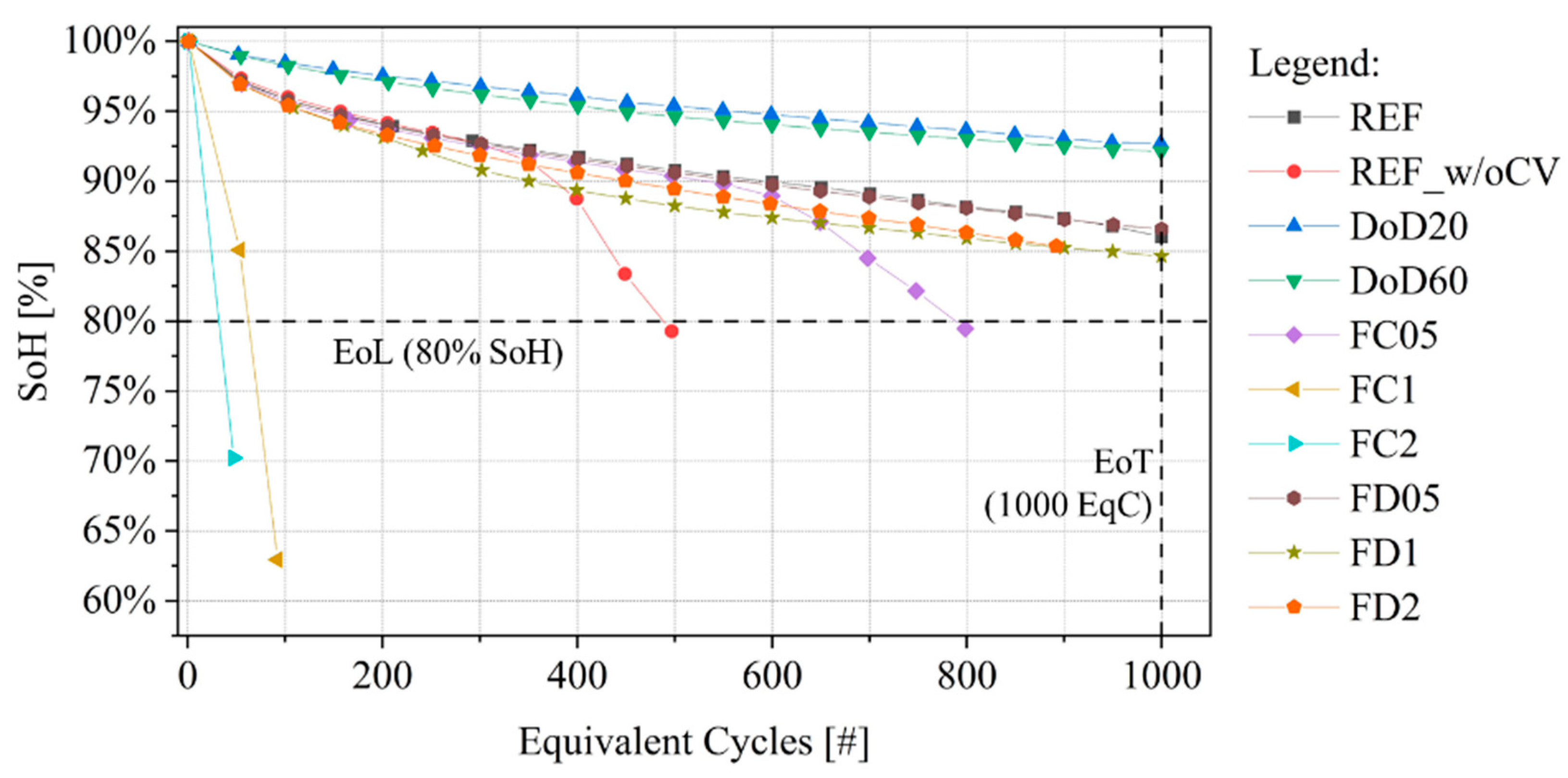
| Cell ID | SoH [%] at EoL/EoT | EqC at EoL/EoT | Pre-Knee SoH Behavior | After-Knee SoH Behavior |
|---|---|---|---|---|
| DOD20 | 92.7% | 1000 | ✓ | ✕ |
| FC05 | 79.5% | 892 | ✓ | ✓ |
| FC1 | 63% | 92 | ✕ | ✓ |
| FD05 | 86.6% | 1000 | ✓ | ✕ |
| FD1 | 84.6% | 1000 | ✓ | ✕ |
| Cell ID | Mean Biased Error [%] | Mean Absolute Error [%] |
|---|---|---|
| DOD60 | 0.69% | 0.73% |
| REF | −0.11% | 0.38% |
| REF_w/oCV | 1.27% | 1.28% |
| FD2 | −1.54% | 1.56% |
| FC2 | −7.46% | 7.46% |
| # | SoH Range | Mean Biased Error [%] | Mean Absolute Error [%] |
|---|---|---|---|
| 1 | 100% > SoH ≥ 95% | −0.05% | 0.38% |
| 2 | 95% > SoH ≥ 90% | 0.01% | 0.40% |
| 3 | 90% > SoH ≥ 85% | 0.43% | 0.71% |
| 4 | 85% > SoH ≥ 80% | 3.57% | 3.65% |
| 5 | SoH < 80% | 0.65% | 6.78% |
Publisher’s Note: MDPI stays neutral with regard to jurisdictional claims in published maps and institutional affiliations. |
© 2022 by the authors. Licensee MDPI, Basel, Switzerland. This article is an open access article distributed under the terms and conditions of the Creative Commons Attribution (CC BY) license (https://creativecommons.org/licenses/by/4.0/).
Share and Cite
Iurilli, P.; Brivio, C.; Carrillo, R.E.; Wood, V. Physics-Based SoH Estimation for Li-Ion Cells. Batteries 2022, 8, 204. https://doi.org/10.3390/batteries8110204
Iurilli P, Brivio C, Carrillo RE, Wood V. Physics-Based SoH Estimation for Li-Ion Cells. Batteries. 2022; 8(11):204. https://doi.org/10.3390/batteries8110204
Chicago/Turabian StyleIurilli, Pietro, Claudio Brivio, Rafael E. Carrillo, and Vanessa Wood. 2022. "Physics-Based SoH Estimation for Li-Ion Cells" Batteries 8, no. 11: 204. https://doi.org/10.3390/batteries8110204