Article

A Generalized Ising-like Model for Spin Crossover Nanoparticles

by
Catherine Cazelles
1,
Jorge Linares
2,3,*,
Pierre-Richard Dahoo
4 and
Kamel Boukheddaden
2,*
1
Université Paris-Saclay, UVSQ, IUT de Mantes en Yvelines, 78200 Mantes la Jolie, France
2
Université Paris-Saclay, UVSQ, CNRS, GEMAC, 78000 Versailles, France
3
Departamento de Ciencias, Sección Física, Pontificia Universidad Católica del Perú, Lima 15088, Peru
4
Université Paris-Saclay, UVSQ, CNRS, LATMOS, 78290 Guyancourt, France
*
Authors to whom correspondence should be addressed.
Magnetochemistry 2022, 8(5), 49; https://doi.org/10.3390/magnetochemistry8050049
Submission received: 14 March 2022 / Revised: 6 April 2022 / Accepted: 7 April 2022 / Published: 4 May 2022

Abstract

:
Cooperative spin crossover (SCO) materials exhibit first-order phase transitions in the solid state, between the high-spin (HS) and low-spin (LS) states. Elastic long-range interactions are the basic mechanism for this particular behavior and are described well by the Ising-like model, which allows the reproduction of most of the experimental results in the literature. Until now, this model has been applied with an interaction parameter between the molecules, which is considered to be independent of the states. In this contribution, we extend the Ising-like model to include interaction energy that depends on the spin states and apply it to study SCO nanoparticles. Our research shows that following this new hypothesis, the equilibrium temperature shifts toward higher values.

1. Introduction

Spin crossover (SCO) nanoparticles [1,2,3,4,5,6,7,8,9,10,11,12] are composed of transition metals with configurations ranging from 3d4 to 3d8 embedded in an organic matrix. They are characterized by two different electronic spin configurations, resulting in two stable, magnetic macrostates, termed high spin (HS) and low spin (LS). LS-HS transitions are triggered by an external constraint. Most of the SCO compounds that have been studied are based on the Fe (II) 3d6 configuration. For the 3d8 case (Ni2+ SCO) and following the work of O.A. Qamar et al. [13], the SCO phenomenon is associated with three different lattice distortions, one of them being from a square planar (LS, S = 0) to a tetrahedral geometry (HS, S = 1).
When a Fe (II) cation coordinates in an octahedral ligand field (Oh) as a metal complex, the degenerated orbitals of the cation split into triply degenerate t2g and doubly degenerate eg states. The macrostates are related to the micro-configurations permitted by the distribution of the six electrons in the t2g and eg states, mediated by the competition between the pairing electron affinity and the strength of the ligand field, which defines the energy gap between the states. The LS state corresponds to the limiting strong field ligand case, which favors the pairing of the six electrons in the t2g orbitals ( t 2 g 6 e g 0 and spin S = 0), and the HS state corresponds to the limiting weak field ligand case, which allows the distribution of the electrons on both the t2g and eg states within the frame of Hund’s rule ( t 2 g 4 e g 2 and total spin S = 2). The LS state is thus diamagnetic when neglecting the second-order Zeeman effect, and the SCO appears in a deeply colored state, while the HS state is a paramagnetic, fainter-colored state. On top of that, the Fe-ligand distance is greater in the HS state compared to the LS state.
The change in spin state can thus be observed through significant changes, such as color, volume, magnetic state and electrical conductivity of the compound from a variety of characterization techniques, including: magnetometry [14,15], Mössbauer spectroscopy [16], optical spectroscopy [17], ellipsometry [18], X-ray diffraction [15,19], calorimetry [20,21], diffuse reflectance [22,23], Raman [15], etc.
From Mössbauer studies, the Debye temperature is observed to be higher for the LS phase than for the HS state. Accordingly, this result suggests that the interactions between the metal complex sites, which are in the LS state, are stronger than those pertaining to interacting HS state sites. This result is in line with a greater HS state Fe-ligand distance. Following these experimental results and conclusions, the theoretical work presented in this contribution is based on an Ising-like model [24,25,26,27,28] that is built on three different coupling parameters to simulate the thermodynamic properties of a SCO solid. Thus, three interaction parameters were introduced: J L L when the two interacting sites are in the LS state, J H H when they are in the HS state and J H L when one site is in the HS state and the other is in the LS state. In the first step, to reduce the number of parameters, the J H L was taken as the average value of the J L L and J H H . Then, the effect of the three different interaction parameters on the equilibrium temperature, as well as on the hysteresis width, were analyzed.
This generalized Ising-like model is presented in Section 2, and the Monte Carlo entropic sampling simulations used to calculate the density of the states are developed in Section 3. The results and analysis are summarized in Section 4.

2. The Model

In the “classical” Ising-like model [24,25], the spin crossover molecules are described by the fictitious operator σ , which has two eigenvalues: +1 assigned to the HS state (with a degeneracy g H S ) and −1 to the LS state (with a degeneracy g L S ). The Hamiltonian for N-isolated molecules is written as:
H = Δ 2     i = 1 N σ i
where ∆ is the gap between the fundamental energies of the HS and LS states. Considering the different degeneracies ( g H S and g L S ) between the respective HS and LS states arising from their different spin values and phonon spectra, the Hamiltonian is isomorphic to:
H = Δ k B T ln g 2 i = 1 N σ i  
with g = g H S g L S , where T is the temperature and k B is the Boltzmann constant.
To account for the interaction between the molecules, an interaction potential energy, written under an Ising form, is added to the previous Hamiltonian, such that:
H = Δ k B T ln g 2   i = 1 N σ i i , j J i j σ i σ j
and considering the presence of short ( J ) and long-range ( G ) interactions, as proposed by Linares et al. [26] and demonstrated later in true elastic models by M. Paez-Espejo et al. [29], the Hamiltonian is finally expressed as
H = Δ k B T ln g 2   i = 1 N σ i     i , j J i j   σ i σ j i = 1 N σ i G σ
which re-writes as
H = Δ k B T ln g G σ 2   i = 1 N σ i     i , j J i j   σ i σ j
where the long-range interaction ( G ) is treated in the mean-field approximation. It is worth remarking that in this contribution, to reduce the parameters, we do not consider different long-range interactions for HS and LS species.
We notice in Equation (5) that the interaction term J i j = J for the nearest molecules (four in the square lattice, six in the cubic lattice) is considered to be independent of the spin states in the “classical” Ising-like model.
In this contribution, we generalize the previous Ising-like model and consider that the short-range interaction term J i j between the sites σ i and σ j depends on their spin states. So, three interaction constants are introduced:
J H H if both molecules are HS, σ i = σ j = + 1 ;
J L L if both molecules are LS, σ i = σ j = 1 ;
J H L if one molecule is HS and the other LS, σ i = σ j = ± 1 .
For the sake of simplicity, it is assumed that J H L = J H H + J L L 2 .
Using the following parameters:
m = i = 1 N σ i ,   s = i , j σ i σ j   and   h = Δ k B T ln g G σ 2
Hamiltonian (5) writes as:
H = h   m     J H H   s H H     J H L   s H L J L L   s L L
where the two-sites’ correlations s H H , s L L and s L L write:
s H H = N + + = i , j σ i σ j ,     for   σ i = σ j = + 1 s L L = N = i , j σ i σ j ,     for   σ i = σ j = 1 s H L = N + + N + = i , j σ i σ j ,     for   σ i = σ j = ± 1
Here, N + + , N and N + are the numbers of the HS-HS, LS-LS and HS-LS nearest neighbor configurations, respectively, which fulfill the relation N + + + N + 2 N + = 2 N , where N is the total number of sites in the considered 2D lattice.
The partition function is then given as a function of these macroscopic variables by:
Z = 1 N d m , s H H , s H L ,   s L L   exp β   h   m J H H s H H J H L s H L J L L s L L
where β = 1 k B   T and d m , s H H , s H L ,   s L L , obtained by the Monte Carlo entropic sampling method (MCES, see Section 3), is the number of configurations with the same m, s H H , s H L   and   s L L values. N is the total number of macrostates characterized by these m, s H H , s H L   and   s L L values.
The thermal average value of the operator σ T , denoted σ , is given by the following relation:
σ = 1 N m     d m , s H H , s H L ,   s L L   exp β   h   m J H H s H H J H L s H L J L L s L L   Z
which is related to the high-spin fraction ( N h s ) by the expression:
N h s = 1 + σ 2
Equation (10) is solved using the bisection technique.

3. Entropic Sampling

The purpose of the Monte Carlo entropic sampling method (MCES) [30,31,32] is to obtain the density of the states d m , s H H , s H L ,   s L L in an attempt to scan the entire space of configurations. To achieve this, the idea is to introduce in the detailed balance equation:
P i   W i j = P j     W j i
Pi the probability of obtaining the macrostate m , s H H , s H L ,   s L L , shown as:
P i = 1 d m i ,   s H H i ,     s H L i ,   s L L i
W i j is the transition probability from the macrostate (i), characterized by mi, (sHH)i, (sHL)i, (sLL)i, to the macrostate (j).
Such a choice of P i   favors the macrostates with a small density of states and dampens those with a high density.
The detailed balance equation is then expressed as:
P m i ,   s H H i ,     s H L i ,   s L L i   W m i ,   s H H i ,     s H L i ,   s L L i m j ,   s H H j ,     s H L j ,   s L L j = P m j ,   s H H j ,     s H L j ,   s L L j   W m j ,   s H H j ,     s H L j ,   s L L j m i ,   s H H i ,     s H L i ,   s L L i
Using d m i ,   s H H i ,   s H L i ,   s L L i as a bias, a “Monte Carlo step” run and a histogram of the frequency of the macrostates H m i ,   s H H i ,   s H L i ,   s L L i are obtained. Then, the density of states in the next “Monte Carlo step” is improved by the following relation:
d m i + 1 ,   s H H i + 1 ,   s H L i + 1 ,   s L L i + 1 = H m i ,   s H H i ,     s H L i ,   s L L i ×   d m i ,   s H H i ,     s H L i ,   s L L i
This technique is used iteratively until an almost constant (flat) H m i ,   s H H i ,   s H L i ,   s L L i histogram is obtained.
The density of states is then used to calculate the thermal average value of the fictitious spin operator.

4. Numerical Results and Analysis

In the calculations, a set of realistic thermodynamic parameters derived from experimental data on the prototype SCO complex [Fe(btr)2(NCS)2], btr = 4,4′-bis-1,2,4-triazole [16] is used. From the enthalpy H measurements, we derived the value of the energy gap as ∆/kB = 1300 K. The equilibrium temperature Teq is deduced from the evolution of ∆H and is fixed at 216.3 K, from which the entropy ∆S = ∆H/Teq is calculated to be ∆S= 50 J/K/mol. Recall that according to the previous model, the expression of Teq is given by T e q = Δ k B ln g .
To study the behavior of SCO molecules, the following definitions are used such that Tup is the ascending thermal transition temperature, Tdown is the descending thermal transition temperature and Teq = T1/2 is the average temperature between Tup and Tdown in which the HS fraction is equal to 1/2. The hysteresis width is defined as Δ T = T u p T d o w n .
In the first part, we study the effect of the interaction parameters on the occurrence of thermal hysteresis and the behavior of its width when it exists. It is worth mentioning that from the experimental point of view, the control of the interactions is usually attempted through metal dilution by replacing a fraction of Fe (II) active SCO atoms with Co, Ni or Zn ions [21,33,34]. Unfortunately, it is usually observed that the effect of the dopant not only breaks down the interactions as expected, but also modulates the ligand field. The results concerning the size effect are given in the second and last parts.
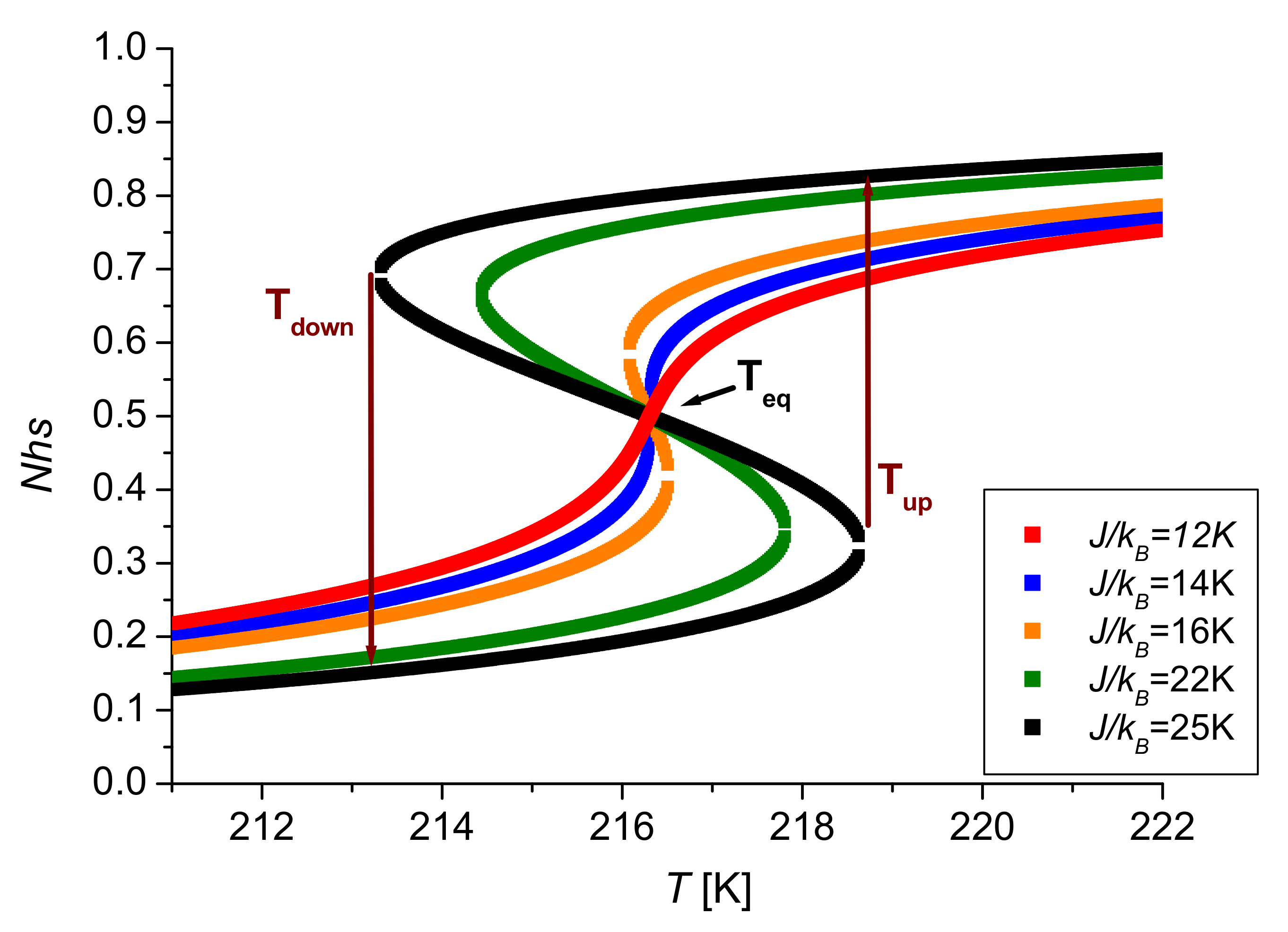
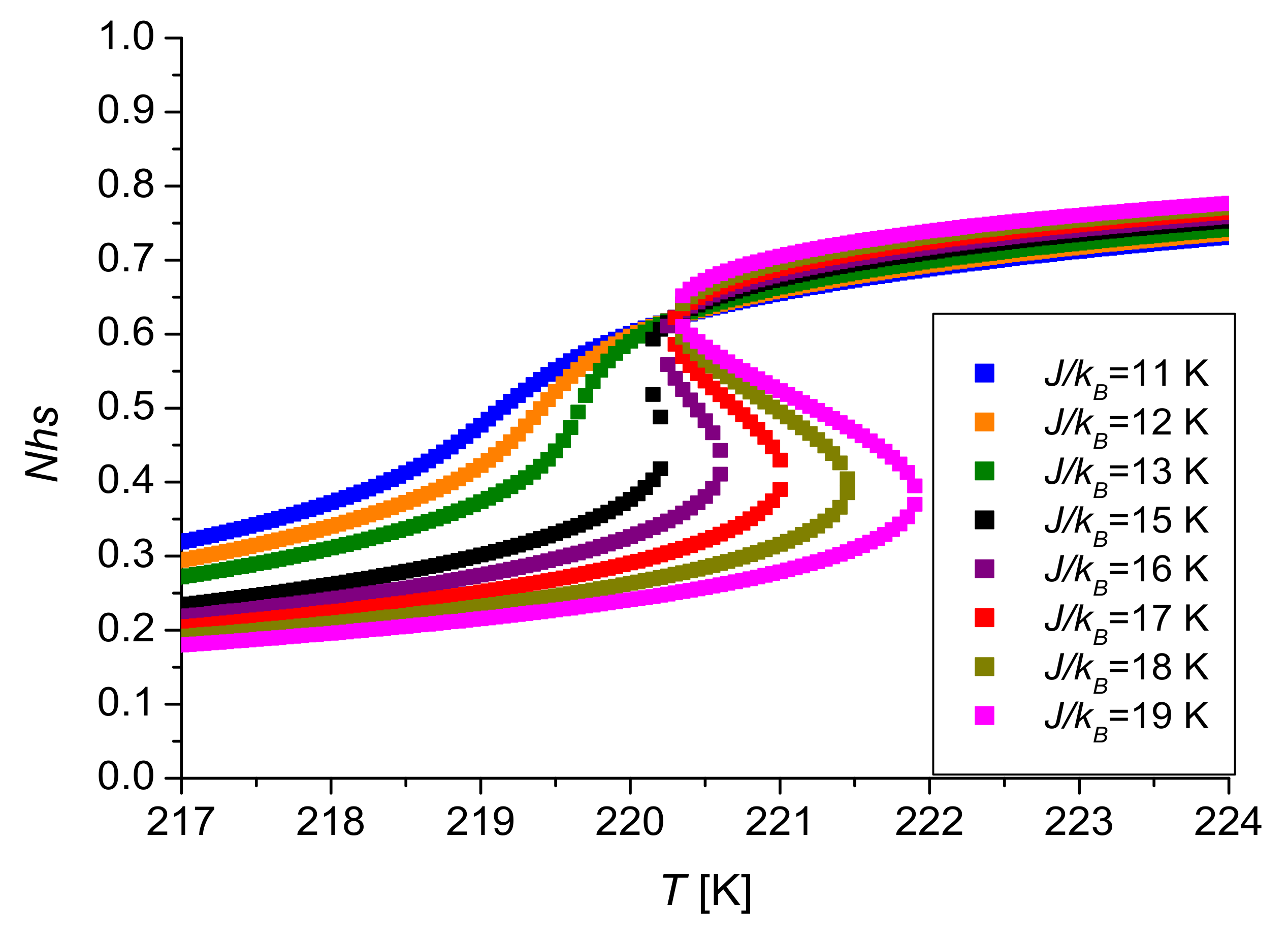
  • Effect of the Interaction Parameters
The effect of the interaction is then simulated by monitoring the value of the effective interaction parameter J / k B .
This “average” interaction parameter is defined here as the usual J parameter of the “classical” Ising-like model, and so it relates to J H H ,   J H L and J L L by the following relation:
J   s =     J H H   s H H     J H L   s H L J L L   s L L
where s = s H H + s L L 2 s H L .
o
The Case x = JHH/JLL = 1.0
Since J H L = J H H + J L L 2 , the case x = 1 corresponds to J H H = J L L = J H L , which will be denoted for simplicity by J . The evolution of the HS fraction, noted as N h s , is simulated as a function of the temperature corresponding to different values of the average short-range parameter J . Figure 1 illustrates the thermal behavior of the HS fraction for various J / k B values ranging from 12 to 25 K.
The curves obtained for the 6 × 6 square system show that the nature of the transition (hysteretic, abrupt or gradual) is closely correlated to the intensity of the short-range interactions.
When the average short-range interaction J / k B is decreased, the thermal hysteresis width reduces from Δ T = 5.41   K ( J / k B = 25   K ) to Δ T = 0.41   K   ( J / k B = 16   K ) and vanishes below the critical value J / k B 15 K . Below this value, the interactions are not strong enough to produce the collective first-order transition accompanied by the hysteretic behavior, and the system’s feature changes into a gradual one, in fair agreement with experimental findings [21,33,34] and previous simulations [26].
Moreover, it can be seen in Figure 1 that when all the interaction parameters J H H / k B , J L L / k B and J H L / k B are equal, the transition temperature Teq is independent of the J / k B values and remains equal to T e q = Δ / k B ln g = 216.3 K.
The previous results are summarized in Figure 2, where we report the phase diagram of the system in the space coordinates T versus J / k B . The presented phase diagram clearly highlights the existence of two regions of thermal behavior: a region corresponding to J / k B 15   K in which the system presents a single first-order phase transition, while a gradual transition is observed when J / k B < 15   K .
o
The Case of x = JHH/JLL = 0.4
The ratio x = J H H / J L L has been set to the value of 0.4, and therefore, the short-range interaction parameters ( J H H , J H L , J L L ) are different. In order to simulate the dilution effect, the intensity of the average short-range interaction J / k B is gradually reduced from J / k B = 19   K to J / k B = 11   K .
The obtained curves are plotted in Figure 3 in the case of a 6 × 6 nanoparticle configuration. The values of the thermal hysteresis widths, as well as the equilibrium temperature T e q , are summarized in Table 1 as a function of the J / k B parameter. The inspection of the thermal behavior of the HS fraction in Figure 3 clearly shows a significant difference compared to Figure 1, which remained symmetric around the invariant value of the transition temperature. Here, the change of the interaction parameter results in a large deformation and shift of N h s T , which means that the interaction J affects both the cooperativity and the ligand field energy.
As can be seen in Table 1, when the interaction parameter J   decreases, the values of J H H / k B and J L L / k B also decrease; the gap J L L J H H / k B decreases as well. An important result is that, at the same time, the thermal hysteresis width decreases, and the equilibrium temperature of the system is shifted to lower temperatures.
In Figure 4, we plot the variations of T u p , T d o w n and T e q  versus  J / k B , which leads to the system’s phase diagram in the ( T , J / k B ) variables’ space, highlighting the existence of two regions of thermal behavior. The thermal hysteresis loop (~1.03 K wide for J / k B = 19   K ), associated with a single first-order phase transition, rapidly narrows when decreasing J / k B and collapses at the threshold value J / k B c 16   K . These results agree qualitatively with Mössbauer spectroscopy and magnetic measurements realized on iron (II)-based SCO materials diluted with high-spin cobalt (II) ions [33,34]. There, the Co has a double role: it breaks down the interactions between the Fe (II) SCO species and also affects the ligand field energy through steric effects.
Linear regression in the Teq(J/kB) variation gives: T ( J / k B ) = 0.24072 × J / k B + 216.30 .
Figure 5 shows the thermal evolution of the HS fraction in the case of a 10 × 10 square lattice. The results are also reported in Table 2. The comparaison of the simulation for 6 × 6 and 10 × 10 square lattices are given in Table 3.
The transition temperatures reported in Figure 6, in the heating mode (Tup) and in the cooling mode (Tdown), clearly show that the width of the hysteresis loop ∆T = Tup − Tdown increases when the J / k B interaction is stronger. Linear regression leads for the Teq Branch to: T ( J / k B ) = 0.26019 × J / k B + 216.30 .
  • Effects of the Variation of x = JHH/JLL
In the following, the value of the ratio x is gradually decreased in the interval [1.0: 0.2]. The value of the J / k B parameter is set to 14.8 K in all simulations. As can be seen in Table 4, when the ratio x = J H H / J L L decreases, the difference between J H H / k B and J L L / k B increases, and the J L L / k B value increases while that of J H H / k B decreases.
The results reported in Figure 7 for a 6 × 6 system show that the decrease in x progressively shifts the equilibrium temperature Teq toward higher values. The equilibrium temperature, which is equal to 216.3 K when x = 1, reaches the value of 221.85 K when x = 0.2 . The values of the equilibrium temperatures associated with the different x values are reported in the last column of Table 4.
In this section, the size effect is analyzed, and calculations are performed in the case of a 10 × 10 square lattice. In the same way, for the 6 × 6 lattice, the value of the ratio x is gradually decreased from the value of 1.0 to the value of 0.2. The results are summarized in Table 5 and in Figure 8 for parameter J / k B set to 14.8 K.
The results of the 10 × 10 lattice are qualitatively similar to those obtained for the 6 × 6 nanoparticle configuration. When the value of the x ratio decreases, the difference between J H H / k B and J L L / k B increases; the interactions between molecules in the LS states ( J L L / k B ) are much stronger than those in the HS state ( J H H / k B ), and the system remains in an LS configuration for a longer temperature interval. The equilibrium temperature Teq gradually moves toward the order-disorder temperature TO.D.. The hysteresis width decreases and vanishes for weaker J / k B values when Teq becomes greater than TO.D..

5. Conclusions

In this study, the behavior of 2D-SCO nanostructures is analyzed with particular attention to the effect of the short-range interactions involved in the model. Indeed, three coupling terms were considered (i) J H H / k B between two HS molecules, (ii) J L L / k B between two LS molecules and (iii) J H L / k B = J / k B between a molecule in the HS state and another one in the LS state with J / k B = J H H / k B + J L L / k B / 2 .
The J H H / J L L ratio effect is parametrized by x . When x = 1 , which corresponds to the case where the three short-range interactions are equal, the equilibrium temperature of the system Teq remains constant. The nature of the transition from LS to HS configuration is governed by the intensity of the interactions and, therefore, the value of the J / k B and G / k B parameters. Increasing the short-range interaction parameter J / k B leads to a hysteretic transition. This behavior is explained by the fact that the Curie (or the order-disorder) temperature designed by TO.D. increases. When x is set to a value other than 1, a “pseudo-dilution” effect is simulated by gradually reducing J / k B . Figure 4 and Figure 6 highlight that the equilibrium temperature shows a linear decrease towards Δ / k B ln g = 216.3 K. Moreover, the hysteretic behavior vanishes at a threshold value of J c / k B 16 K and J c / k B 15 K for 6 × 6 and 10 × 10 systems, respectively. This feature is connected to the relative positions of Teq and TO.D. and can be explained by the fact that the order-disorder transition TO.D. decreases faster for small lattices. The condition Teq > TO.D. leads to a gradual transition. In the present study, we mainly focused on the effect of varying x when J / k B is constant. An important result is that when the difference between J H H / k B and J L L / k B is increased, the LS state is stabilized and Teq is shifted toward higher temperatures. This behavior is more significant for larger lattices. The effects of the interactions between surface molecules and their environment will also be explored in future work.

Author Contributions

J.L. and K.B. proposed the model, C.C. and J.L. calculated the density of states and conducted the simulations, J.L., K.B., C.C. and P.-R.D. analyzed the results. All the authors participated in writing the paper. All authors have read and agreed to the published version of the manuscript.

Funding

This research received no external funding.

Institutional Review Board Statement

Not applicable.

Informed Consent Statement

Not applicable.

Data Availability Statement

Not applicable.

Acknowledgments

This research was funded by the CNRS and the Université de Versailles St-Quentin member of the Université Paris-Saclay, the ANR project Mol-CoSM No. ANR-20-CE07-0028-02 and the French–Japan international laboratory (LIA IM-LED). We thank all of them for their financial support.

Conflicts of Interest

The authors declare no conflict of interest.

References

  1. Coronado, E. Molecular magnetism: From chemical design to spin control in molecules, materials and devices. Nat. Rev. Mater. 2020, 5, 87–104. [Google Scholar] [CrossRef]
  2. Gütlich, P.; Hauser, A.; Spiering, H. Thermal and optical switching of Iron(II) Complexes. Angew. Chem. 1994, 33, 2024–2054. [Google Scholar] [CrossRef]
  3. Sanvito, S. Molecular Spintronics. Chem. Soc. Rev. 2011, 40, 3336–3355. [Google Scholar] [CrossRef] [PubMed]
  4. Decurtins, S.; Gütlich, P.; Köhler, C.P.; Spiering, H.; Hauser, A. Light-induced excited spin state trapping in a transition-metal complex: The hexa-1-propyltetrazole-iron (II) tetrafluoroborate spin-crossover system. Chem. Phys. Lett. 1984, 105, 1–4. [Google Scholar] [CrossRef]
  5. Linares, J.; Codjovi, E.; Garcia, Y. Pressure and Temperature Spin Crossover Sensors with Optical Detection. Sensors 2012, 12, 4479–4492. [Google Scholar] [CrossRef]
  6. Boukheddaden, K.; Ritti, M.H.; Bouchez, G.; Sy, M.; Dîrtu, M.M.; Parlier, M.; Linares, J.; Garcia, Y. Quantitative contact pressure sensor based on spin crossover mechanism for civil security applications. J. Phys. Chem. C 2018, 122, 7597–7604. [Google Scholar] [CrossRef]
  7. Spiering, H. Elastic interaction in spin-crossover compounds. In Spin Crossover in Transition Metal Compounds III Topics in Current Chemistry; Springer: Berlin/Heidelberg, Germany, 2004; Volume 235, pp. 171–195. [Google Scholar] [CrossRef]
  8. Boukheddaden, K.; Linares, J.; Spiering, H.; Varret, F. One-dimensional Ising-like systems: An analytical investigation of the static and dynamic properties, applied to spin-crossover relaxation. Eur. Phys. J. B 2000, 15, 317–326. [Google Scholar] [CrossRef]
  9. Boukheddaden, K.; Linares, J.; Varret, F. Thermodynamic properties of coupled mixed-valence molecules using a cooperative PKS theory: A second-order localized-delocalized transition. Chem. Phys. 1993, 172, 239–245. [Google Scholar] [CrossRef]
  10. Constant-Machado, H.; Stancu, A.; Linares, J.; Varret, F. Thermal hysteresis loops in spin-crossover compounds analyzed in terms of classical Preisach model. IEEE Trans. Mag. 1998, 34, 2213–2219. [Google Scholar] [CrossRef]
  11. Linares, J.; Jureschi, C.M.; Boukheddaden, K. Surface effects leading to unusual size dependence of the thermal hysteresis behavior in spin-crossover nanoparticles. Magnetochemistry 2016, 2, 24. [Google Scholar] [CrossRef] [Green Version]
  12. Rotaru, A.; Linares, J.; Varret, F.; Codjovi, E.; Slimani, A.; Tanasa, R.; Enachescu, C.; Stancu, A.; Haasnoot, J. Pressure effect investigated with first-order reversal-curve method on the spin-transition compounds [FexZn1−x(btr)2(NCS)2] ·H2O (x = 0.6,1). Phys. Rev. B 2011, 83, 224107–224114. [Google Scholar] [CrossRef]
  13. Qamar, O.A.; Cong, C.; Ma, H. Solid state mononuclear divalent nickel spin crossover complexes. Dalton Trans. 2020, 49, 17106–17114. [Google Scholar] [CrossRef] [PubMed]
  14. Kahn, O. Molecular Magnetism; Wiley-VCH: New York, NY, USA, 1993. [Google Scholar]
  15. Shepherd, H.J.; Bonnet, S.; Guionneau, P.; Bedoui, S.; Garbarino, G.; Nicolazzi, W.; Bousseksou, A.; Molnar, G. Pressure-induced two-step transition with structural symmetry breaking: X-ray diffraction, magnetic, and Ramman studies. Phys. Rev. B 2011, 54, 144107–144115. [Google Scholar] [CrossRef] [Green Version]
  16. Krober, J.; Audière, J.P.; Claude, R.; Codjovi, E.; Kahn, O.; Hassnoot, J.; Grolière, F.; Jay, C.; Bousseksou, A.; Linares, J.; et al. Spin Transitions and Thermal Hysteresis in the Molecular-Based Materials [Fe(Htrz)2(trz)](BF4) and [Fe(Htrz)3](BF4)2.cntdot.H2O (Htrz = 1,2,4-4H-triazole; trz = 1,2,4-triazolato). Chem. Mater. 1994, 6, 1404–1412. [Google Scholar] [CrossRef]
  17. Varret, F.; Slimani, A.; Boukheddaden, K.; Chong, C.; Mishra, H.; Collet, E.; Haasnoot, J.; Pillet, S. The Propagation of the Thermal Spin Transition of [Fe(Btr)2(NCS)2]_H2O Single Crystals Observed by Optical Microscopy. New J. Chem. 2011, 35, 2333–2340. [Google Scholar] [CrossRef]
  18. Loutete-Dangui, E.D.; Codjovi, E.; Tokoro, H.; Dahoo, P.R.; Ohkoshi, S.; Boukheddaden, K. Spectroscopic ellipsometry investigations of the thermally induced first-order transition of RbMn[Fe(CN)6]. Phys. Rev. B 2008, 78, 014303–014312. [Google Scholar] [CrossRef]
  19. Pillet, S.; Hubsch, J.; Lecomte, C. Single crystal diffraction analysis of the thermal spin conversion in [Fe(btr)2(NCS)2](H2O): Evidence for spin-like domain formation. Eur. Phys. J. B 2004, 38, 541–552. [Google Scholar] [CrossRef]
  20. Roubeau, O.; Castro, M.; Burriel, R.; Haasnoot, J.G.; Reedijk, J. Calorimetric Investigation of Triazole-Bridged Fe(II) Spin-Crossover One-Dimensional Materials: Measuring the Cooperativity. J. Phys. Chem. B 2011, 115, 3003–3012. [Google Scholar] [CrossRef]
  21. Rotaru, A.; Dîrtu, M.M.; Enachescu, C.; Tanasa, R.; Linares, J.; Stancu, A.; Garcia, Y. Calorimetric measurements of diluted spin crossover complexes [FexM1−x(btr)2(NCS)2]·H2O with MII = Zn and Ni. Polyhedron 2009, 28, 2531–2536. [Google Scholar] [CrossRef]
  22. Rotaru, A.; Varret, F.; Codjovi, E.; Boukheddaden, K.; Linares, J.; Stancu, A.; Guionneau, P.; Létard, J.F. Hydrostatic pressure investigation of the spin crossover compound [Fe(PM-BIA)2(NCS)2] polymorph I using reflectance detection. J. Appl. Phys. 2009, 106, 053515–053520. [Google Scholar] [CrossRef]
  23. Rotaru, G.M.; Codjovi, E.; Dahoo, P.R.; Maurin, I.; Linares, J.; Rotaru, A. Monotoring-Spin-Crossover Properties by Diffussed Reflectivity. Symmetry 2021, 13, 1148. [Google Scholar] [CrossRef]
  24. Wajnflasz, J.; Pick, R. Transitions “low spin”—“high spin” dans les complexes de Fe2+. J. Phys. Colloques 1971, 32, 91–92. [Google Scholar] [CrossRef]
  25. Bousseksou, A.; Nasser, J.; Linares, J.; Boukheddaden, K.; Varret, F. Ising-like model for the two-step spin-crossover. J. Phys. I France 1992, 2, 1381–1403. [Google Scholar] [CrossRef]
  26. Linares, J.; Spiering, H.; Varret, F. Analytical solution of 1d ising-like systems modified by weak long-range interaction—Application to spin crossover compounds. Eur. Phys. J. B 1999, 10, 271–275. [Google Scholar] [CrossRef]
  27. Chiruta, D.; Jureschi, C.-M.; Linares, J.; Dahoo, P.R.; Garcia, Y.; Rotaru, A. On the origin of multi-step spin transition behaviour in 1d nanoparticles. Eur. Phys. J. B 2015, 88, 233. [Google Scholar] [CrossRef]
  28. Ndiaye, M.; Singh, Y.; Fourati, H.; Sy, M.; Lo, B.; Boukheddaden, K. Isomorphism between the electro-elastic modeling of the spin transition and Ising-like model with competing interactions: Elastic generation of self-organized spin states. J. App. Phys. 2021, 129, 153901–153921. [Google Scholar] [CrossRef]
  29. Paez-Espejo, M.; Sy, M.; Boukheddaden, K. Elastic frustration causing two-step and multistep transitions in spin crossover solids: Emergence of complex Aantiferroelastic structures. J. Am. Chem. Soc. 2016, 138, 3202–3210. [Google Scholar] [CrossRef]
  30. Shteto, I.; Linares, J.; Varret, F. Monte carlo entropic sampling for the study of metastable states and relaxation paths. Phys. Rev. E 1997, 56, 5128–5137. [Google Scholar] [CrossRef]
  31. Linares, J.; Cazelles, C.; Dahoo, P.R.; Boukheddaden, K. A first-order phase transition studied by an Ising-like model solved by entropic Sampling Monte Carlo Method. Symmetry 2021, 13, 587. [Google Scholar] [CrossRef]
  32. Linares, J.; Enachescu, C.; Boukheddaden, K.; Varret, F. Monte Carlo entropic sampling applied to spin crossover solids: The squareness of the thermal hysteresis loop. Polyhedron 2003, 22, 2453–2456. [Google Scholar] [CrossRef]
  33. Constant-Machado, H.; Linares, J.; Varret, F.; Haasnoot, J.G.; Martin, J.P.; Zarembowitch, J.; Dworkin, A.; Bousseksou, A. Dilution effects in a spin crossover system, modelled in terms of direct and indirect intermolecular interactions. J. Phys. I Fr. 1996, 6, 1203–1216. [Google Scholar] [CrossRef] [Green Version]
  34. Martin, J.P.; Zarembowitch, J.; Bousseksou, A.; Dworkin, A.; Haasnoot, J.G.; Varret, F. Solid State Effects on Spin Transitions: Magnetic, Calorimetric, and Moessbauer-Effect Properties of [FexCo1−x(4,4′-bis-1,2,4-triazole)2(NCS)2].cntdot.H2O Mixed-Crystal Compounds. Inorg. Chem. 1994, 33, 6325–6333. [Google Scholar] [CrossRef]
Figure 1. Thermal evolution of the HS fraction in a SCO system with a size of 6 × 6 for different values of the average interaction parameter J / k B : J / k B = 12   K (red square), J / k B   = 14 K (blue square), J / k B = 16 K (orange square), J / k B = 22 K (green square) and J / k B = 25 K (black square). The computational parameters are: Δ / k B = 1300 K, G / k B = 172.2 K, x =   J H H / J L L = 1.0 and ln(g) = 6.01.
Magnetochemistry 08 00049 g001
Figure 2. Phase diagram T = f (J/kB) for a 6 × 6 square lattice. The red and blue squares correspond, respectively, to the upper and lower transitions for the heating (Tup) and cooling (Tdown) temperatures of the thermal HS fraction. The black squares correspond to the equilibrium temperatures (Teq). The computational parameters are: Δ / k B = 1300 K, G / k B = 172.2 K, x = J H H / J L L = 1.0 and ln(g) = 6.01.
Magnetochemistry 08 00049 g002
Figure 3. Thermal evolution of the HS fraction in a SCO system with a size of 6 × 6 for different values of the average interaction parameter J / k B : J / k B = 19 K (magenta square), J / k B = 18 K (dark yellow square), J / k B = 17 K (red square), J / k B = 16 K (purple square), J / k B = 15 K (black square), J / k B = 13 K (green square), J / k B = 12 K (orange square) and J / k B = 11 K (blue square). The computational parameters are: Δ / k B   = 1300 K, G / k B = 172.2 K, x = J H H / J L L = 0.4 and ln(g) = 6.01.
Magnetochemistry 08 00049 g003
Figure 4. Temperature T versus J/kB for a 6 × 6 square lattice. The red (Tup) and blue (Tdown) squares correspond, respectively, to the transition temperatures of the upper and lower branches of thermal hysteresis. The black squares correspond to the equilibrium temperatures (Teq) of the gradual transition region. The computational parameters are: Δ / k B = 1300 K, G / k B = 172.2 K, x = ( J H H / k B ) / ( J L L / k B ) = 0.4 and ln(g) = 6.01.
Magnetochemistry 08 00049 g004
Figure 5. Thermal evolution of the HS fraction in a SCO system with a size of 10 × 10 for different values of the average interaction parameter J / k B : J / k B = 19 K (magenta square), J / k B = 18 K (dark yellow square), J / k B = 17 K (red square), J / k B = 16 K (purple square), J / k B = 15 K (black square), J / k B = 13 K (green square), J / k B = 12 K (orange square), J / k B = 11 K (blue square). The computational parameters are: Δ / k B   = 1300 K, G / k B = 172.2 K, x = J H H / J L L = 0.4 and ln(g) = 6.01.
Magnetochemistry 08 00049 g005
Figure 6. Phase diagram T = f (J/kB) for a 10 × 10 square lattice. The red and blue squares correspond, respectively, to the upper and lower transitions for the heating (Tup) and cooling (Tdown) temperatures of the thermal HS fraction. The black squares correspond to the equilibrium temperatures (Teq). The computational parameters are: Δ / k B = 1300 K, G / k B = 172.2 K, x = ( J H H / J L L ) = 0.4 and ln(g) = 6.01.
Magnetochemistry 08 00049 g006
Figure 7. Thermal evolution of the HS fraction in a SCO system with a size of 6 × 6 for different values of the x parameter: x = 1.0 (green square), x = 0.6 (purple square) and x = 0.2 (red square). The computational parameters are: Δ / k B = 1300 K, J / k B = 14.8 K, G / k B = 172.2 K and ln(g) = 6.01.
Magnetochemistry 08 00049 g007
Figure 8. Thermal evolution of the HS fraction in a SCO system with a size of 10 × 10 for different values of the x parameter: x = 0.2 (red square), x = 0.6 (purple square) and x = 1.0 (green square). The computational parameters are: Δ / k B = 1300 K, J / k B = 14.8 K, G / k B = 172.2 K and ln(g) = 6.01.
Magnetochemistry 08 00049 g008
Table 1. Values of the thermal hysteresis width Δ T h y s t = T u p T d o w n and the equilibrium temperature T e q as a function of J / k B , J H H / k B and J L L / k B in a SCO system with a size of 6 × 6. The computational parameters are: Δ / k B = 1300 K, G / k B = 172.2 K, x = J H H / J L L = 0.4 and ln(g) = 6.01.
J / k B   K J H H / k B   [ K ] J L L / k B   [ K ] J L L J H H / k B   K Δ T h y s t   K T e q   [ K ]
1910.8627.1416.281.03220.86
1810.2825.7115.430.62220.60
179.7224.2914.570.33220.37
169.1422.8613.720.10220.13
158.5721.4312.860219.90
137.4318.5811.150219.43
126.8517.1410.290219.18
116.2815.719.420218.93
Table 2. Evolution of the thermal hysteresis width, Δ T h y s t = T u p T d o w n , and the equilibrium temperature, T e q , as a function of J / k B , J H H / k B and J L L / k B in a SCO system with a size of 10 × 10. The computational parameters are: Δ / k B = 1300 K, G / k B = 172.2 K, x = J H H / J L L and ln(g) = 6.01.
J / k B   K J H H / k B   [ K ] J L L / k B   [ K ] ( J L L / k B J H H / k B )   K Δ T h y s t   K   10   ×   10 T e q   [ K ]   10   ×   10
1910.83727.09416.2571.57221.244
1810.26725.66915.4021.13220.941
179.69724.24414.5470.71220.709
169.12522.81413.6890.38220.463
158.55521.38912.8340.09220.160
137.41518.53911.1240219.658
126.84517.11410.2690219.409
116.27415.6859?4110219.149
Table 3. Comparison of simulations for the 6 × 6 and 10 × 10 lattices.
J / k B   K Δ T h y s t   K   6   ×   6 T e q   [ K ]   6   ×   6 Δ T h y s t   K   10   ×   10 T e q   [ K ]   10   ×   10
191.03220.861.57221.244
180.62220.601.13220.941
170.33220.370.71220.709
160.10220.130.38220.463
150219.900.09220.160
130219.430219.658
120219.180219.409
110218.930219.149
Table 4. Equilibrium temperatures and hysteresis widths calculated for different values of x = J H H / J L L parameter in a 6 × 6 square lattice. The computational parameters are: Δ / k B = 1300 K, J / k B = 14.8 K, G / k B = 172.2 K and ln(g) = 6.01.
J / k B   [ K ] x J L L / k B   [ K ] J H H / k B   [ K ] J H L / k B   [ K ] Δ T h y s t   [ K ] T e q   [ K ]
14.81.014.814.814.80.11216.30
14.80.618.511.0914.80218.38
14.80.224.664.9314.80221.85
Table 5. Equilibrium temperatures and hysteresis widths calculated for different values of the x = ( J H H / k B ) / ( J L L / k B ) parameter in a 10 × 10 square lattice. The computational parameters are: Δ / k B = 1300 K, J / k B = 14.8 K, G / k B = 172.2 K and ln(g) = 6.01.
J / k B   [ K ] x J L L / k B   [ K ] J H H / k B   [ K ] J H L / k B   [ K ] Δ T h y s t   [ K ] T e q   [ K ]
14.81.014.814.814.86.10216.30
14.80.618.4811.08714.785.16219.88
14.80.224.594.9214.750222.29
Publisher’s Note: MDPI stays neutral with regard to jurisdictional claims in published maps and institutional affiliations.

