
Physiological Disorder Diagnosis of Plant Leaves Based on Full-Spectrum Hyperspectral Images with Convolutional Neural Network


Abstract
:1. Introduction
2. Materials and Methods
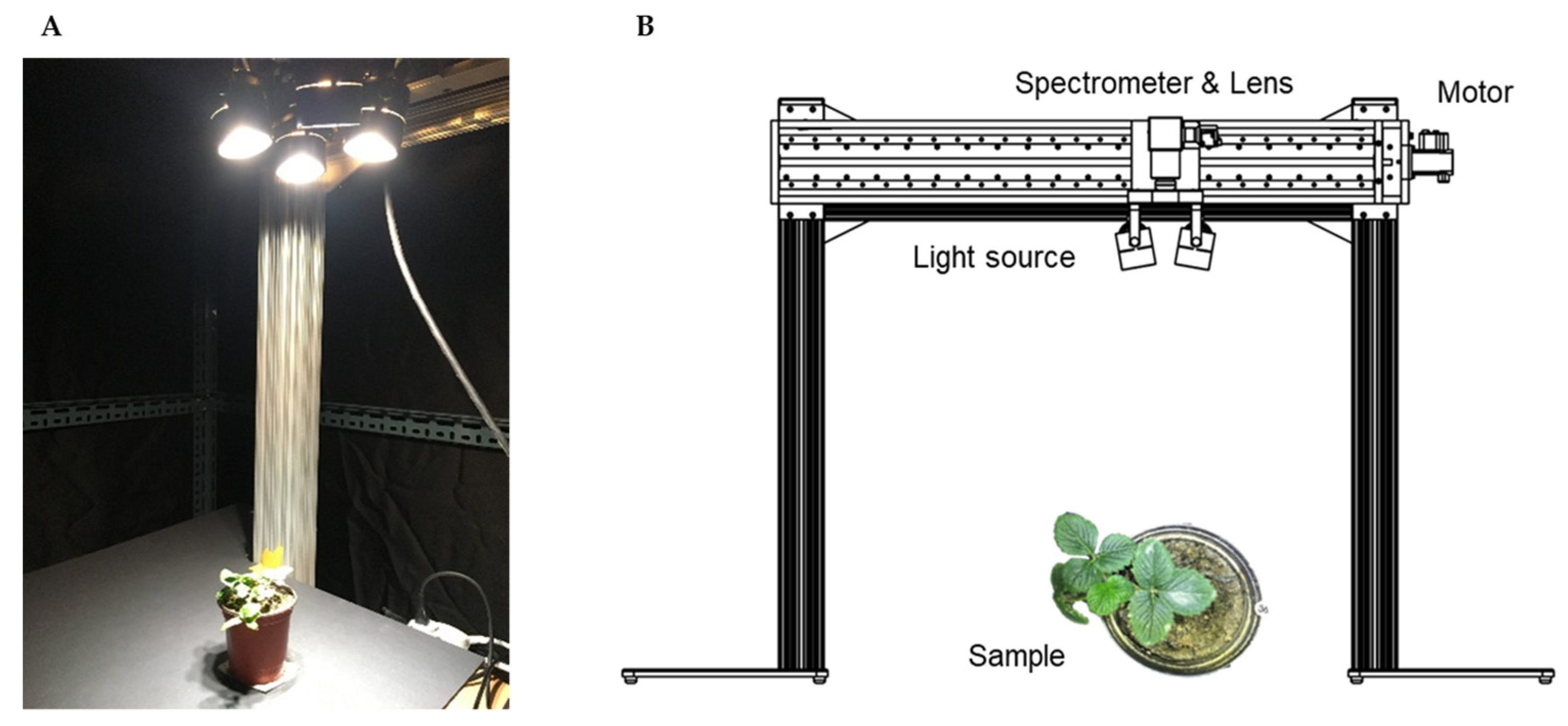
2.1. Hyperspectral Imaging System
2.1.1. 3D Crop Extraction
2.1.2. Hyperspectral Image Calibration
2.2. Data Acquisition and Plant Physiological Disorder Samples
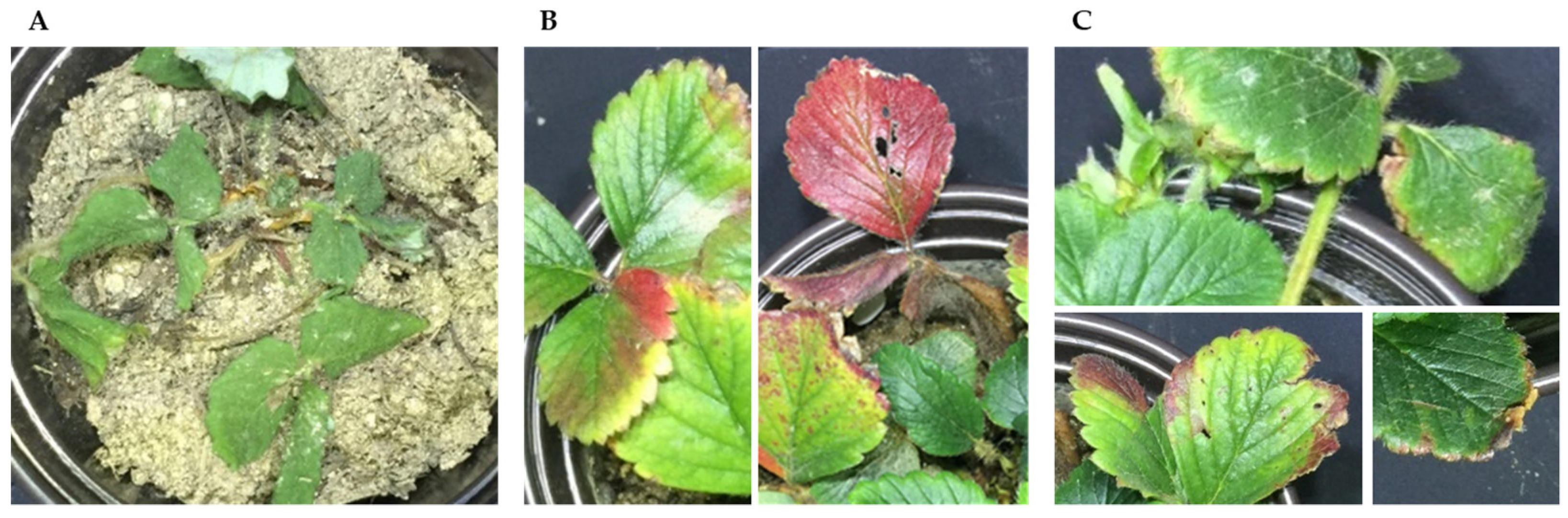
2.2.1. Target Crops and Physiological Disorders
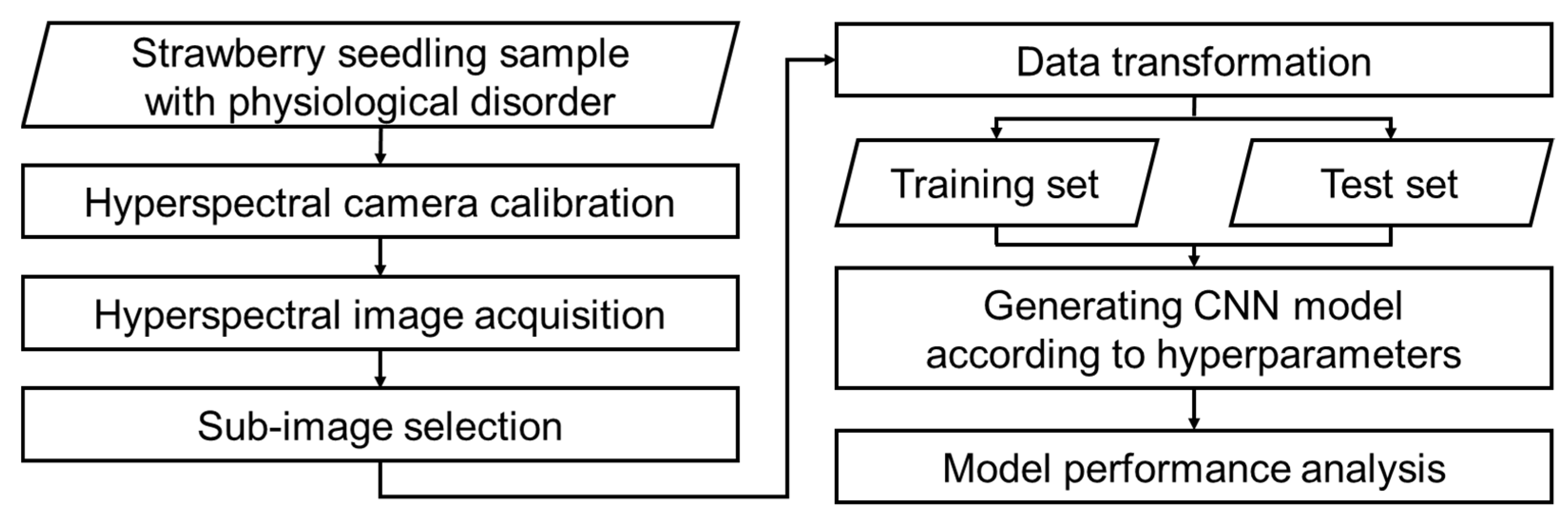
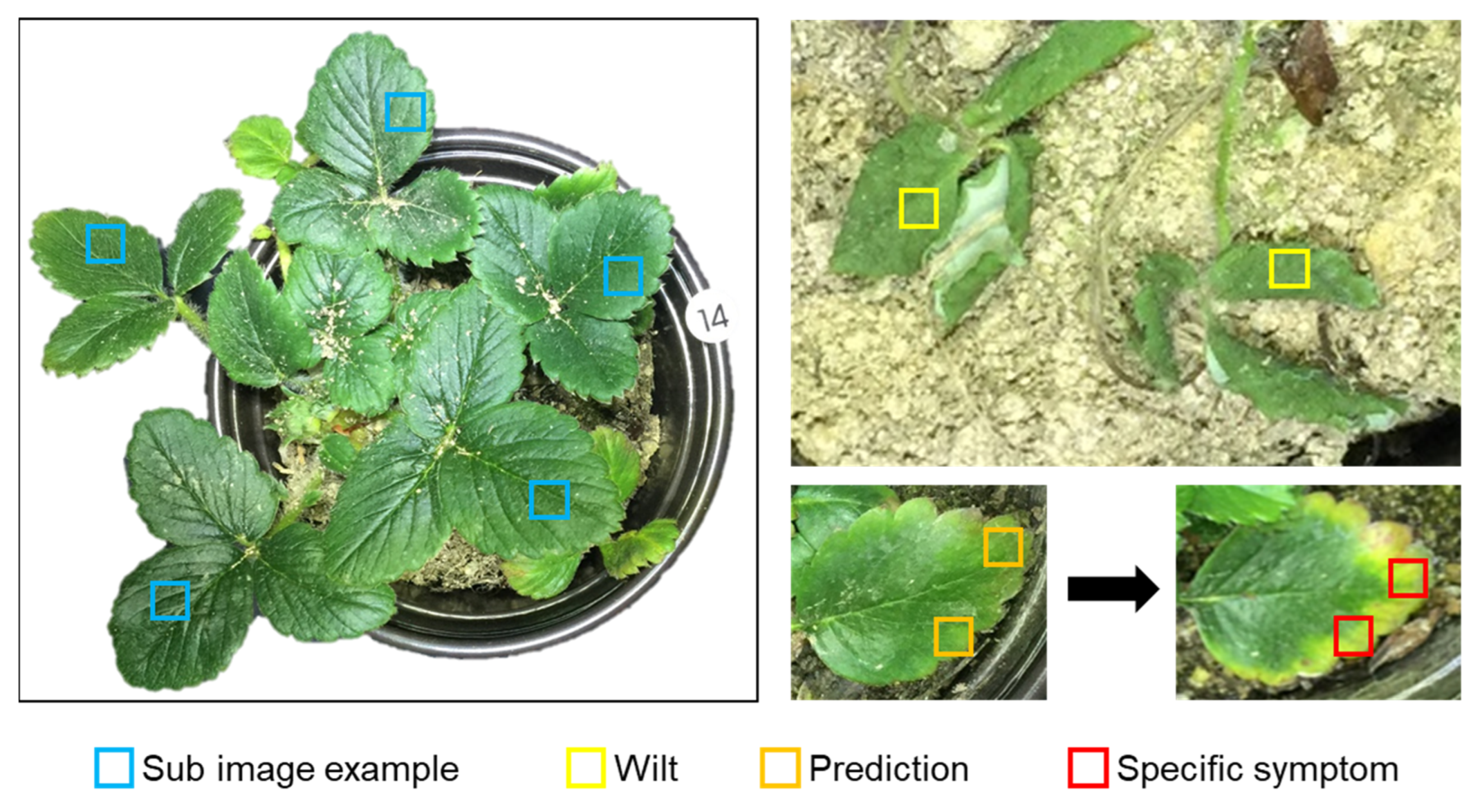
2.2.2. Data Preprocessing
2.3. Deep Learning-Based Diagnosis Technology
2.3.1. Diagnosis Model
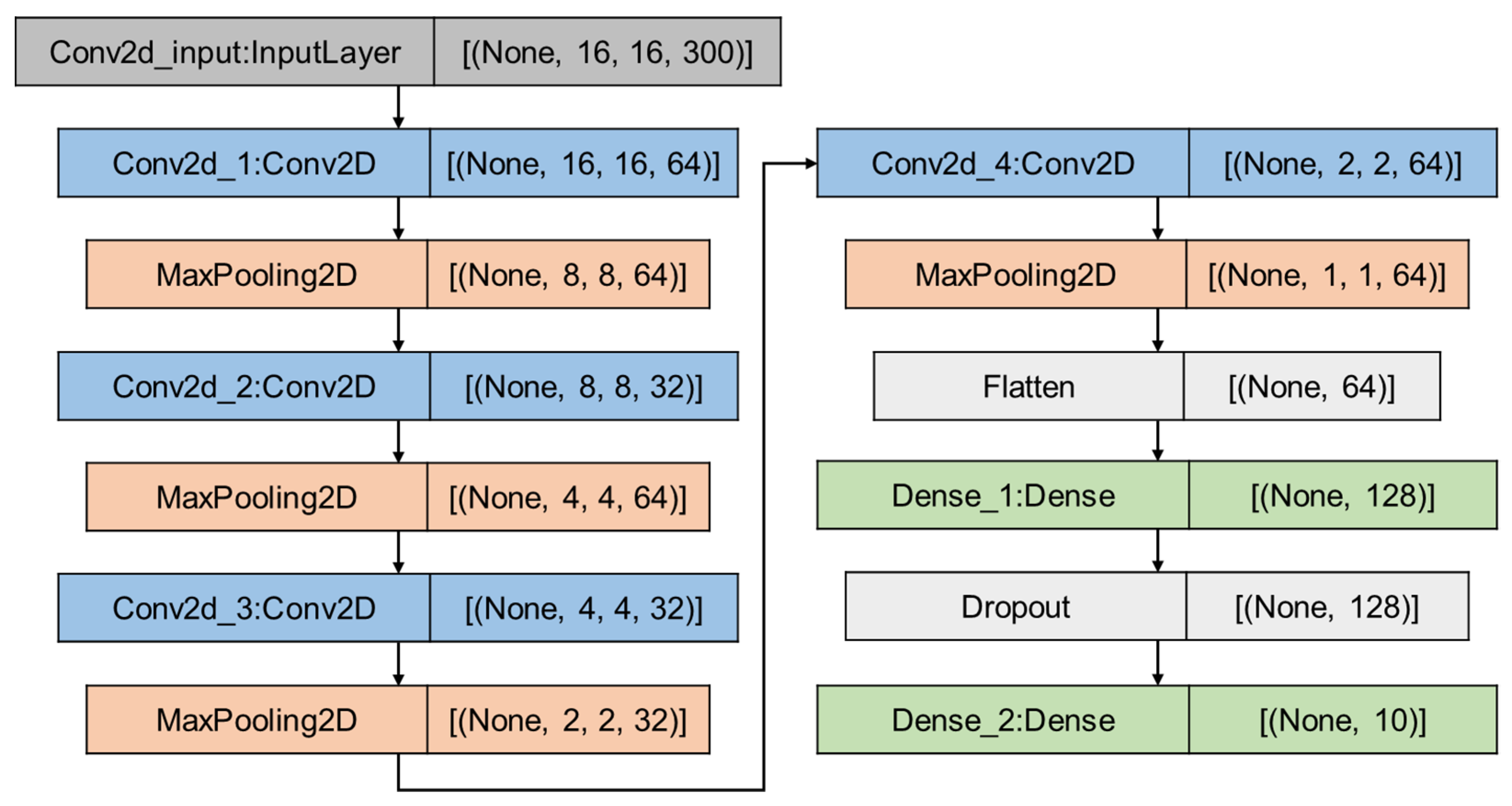
2.3.2. CNN Architecture
2.3.3. Utilized Optimizer
- Stochastic Gradient Descent
- Adaptive Gradient
- Root Mean Square Propagation
- Adaptive Moment Estimation
2.3.4. Performance Evaluation Index
3. Results and Discussion
3.1. Model Learning Time and Accuracy
3.2. Analysis According to the Optimizers
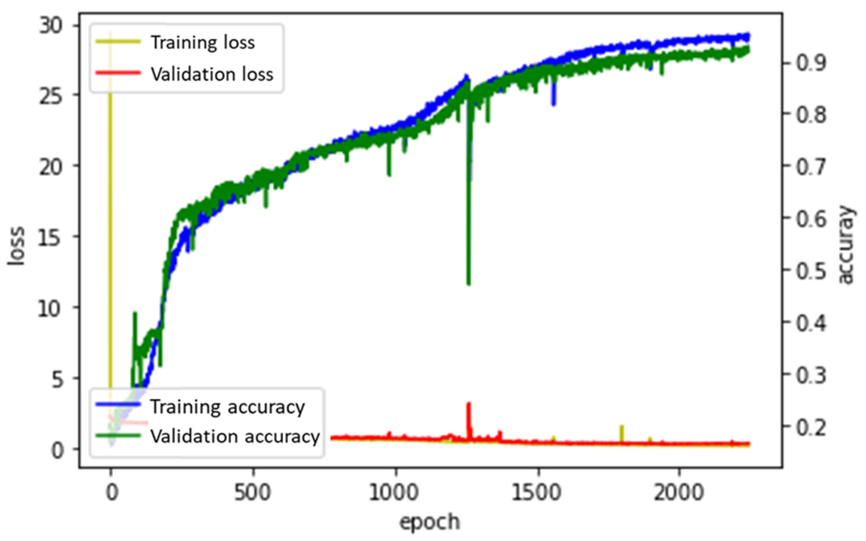
3.2.1. Adagrad
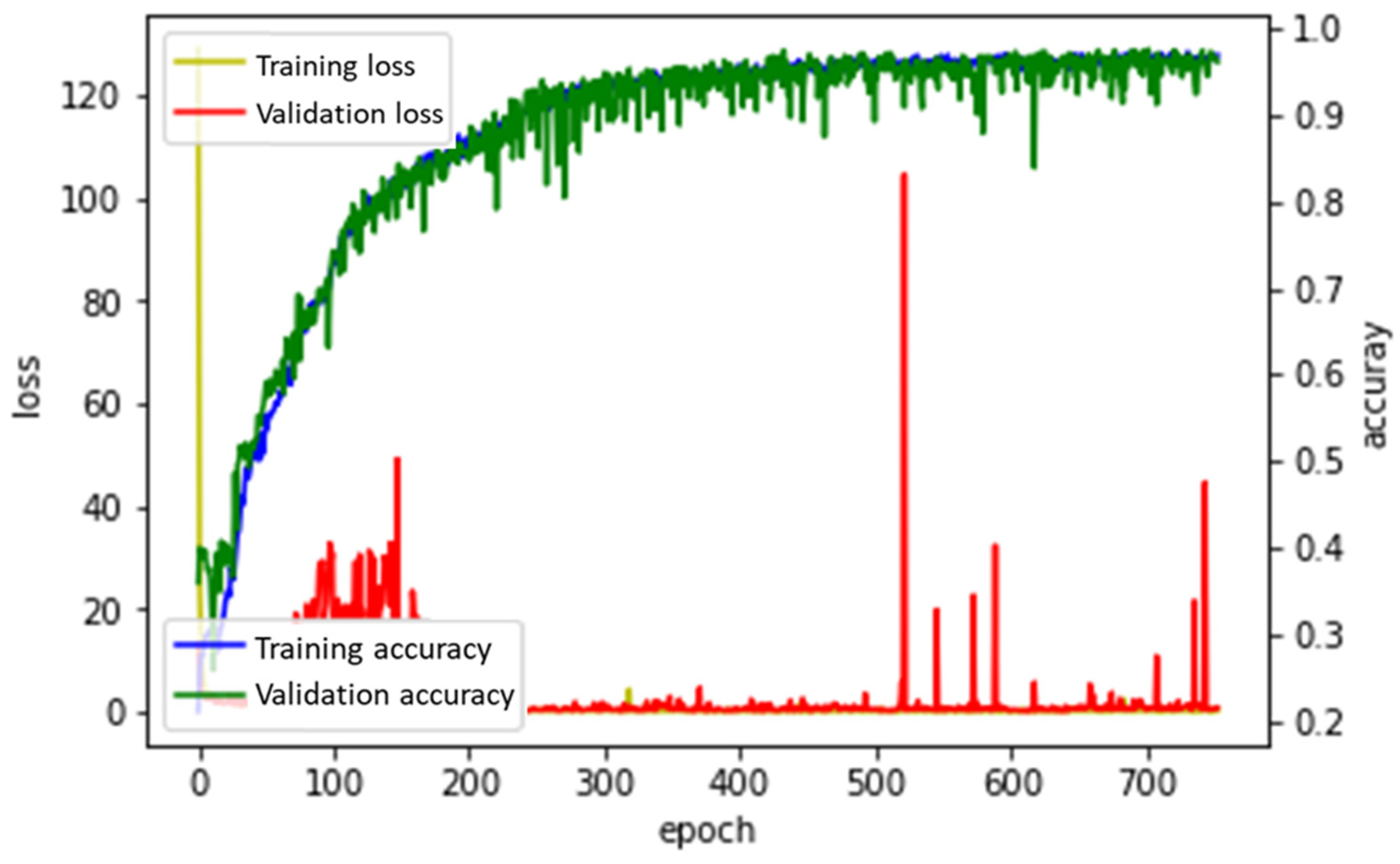
3.2.2. RMSProp
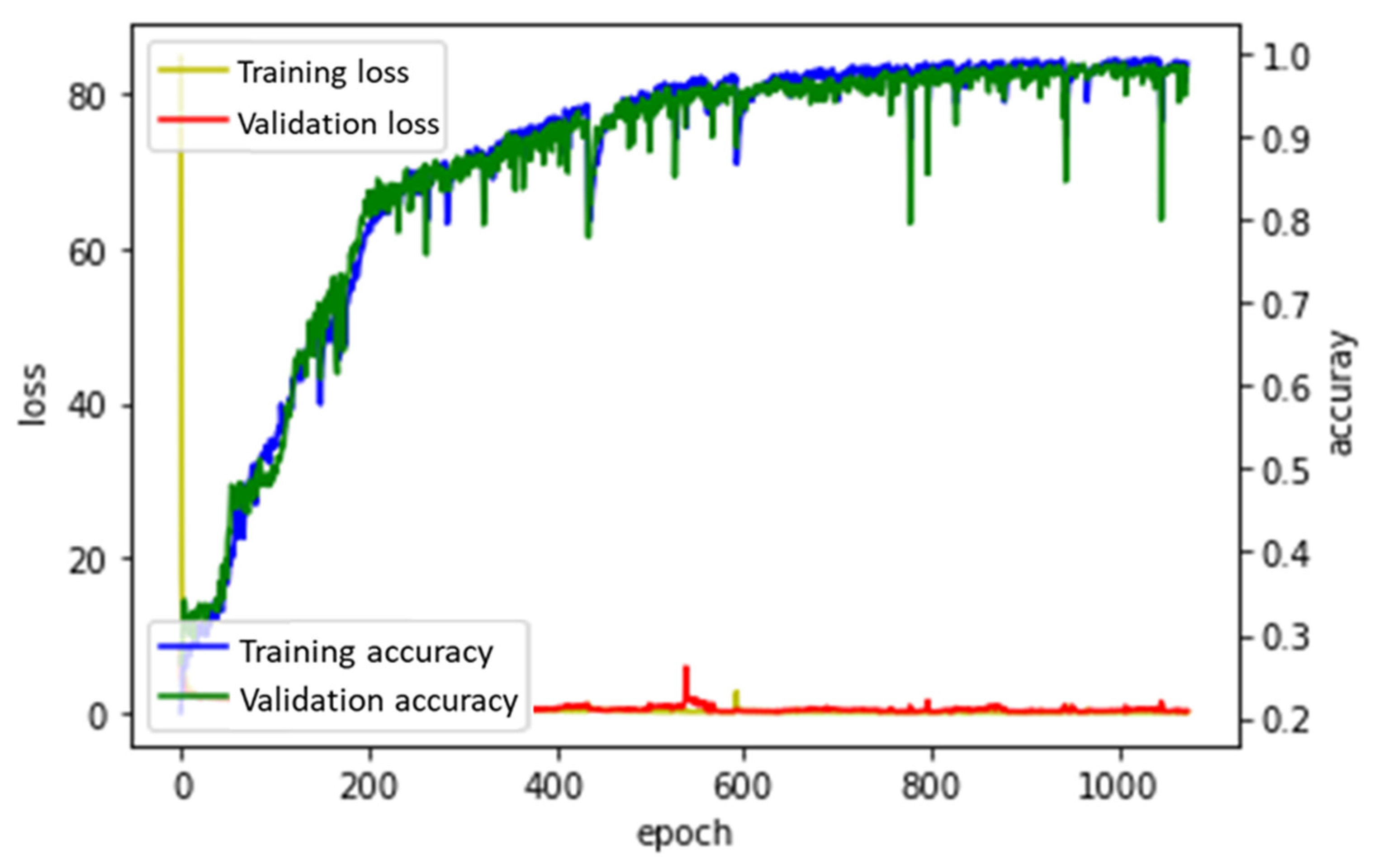
3.2.3. Adam
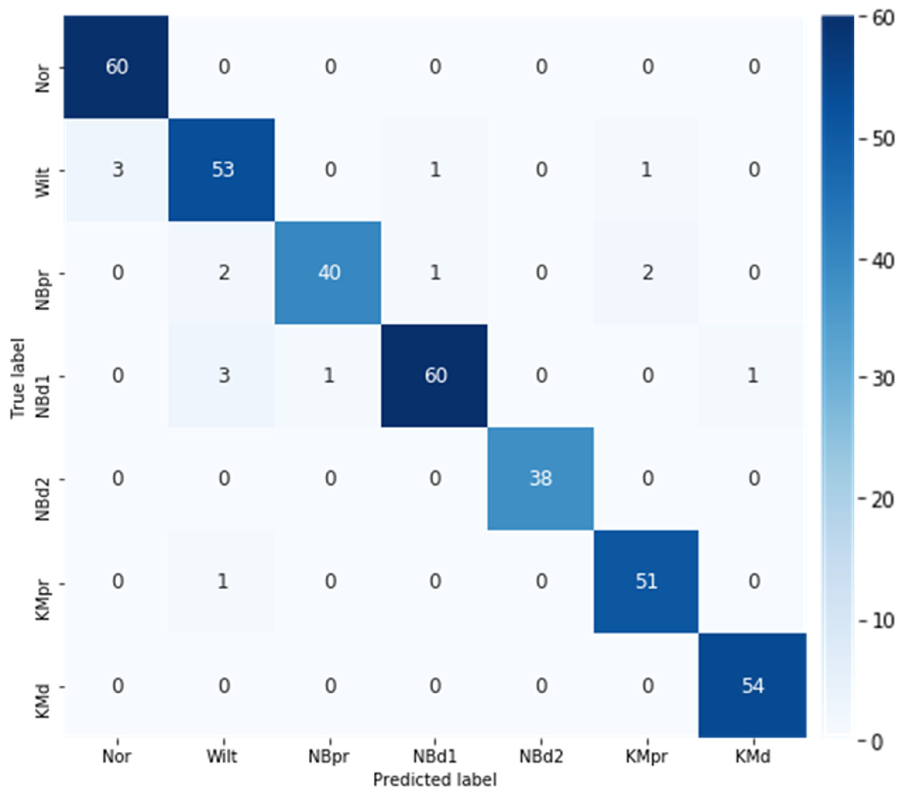
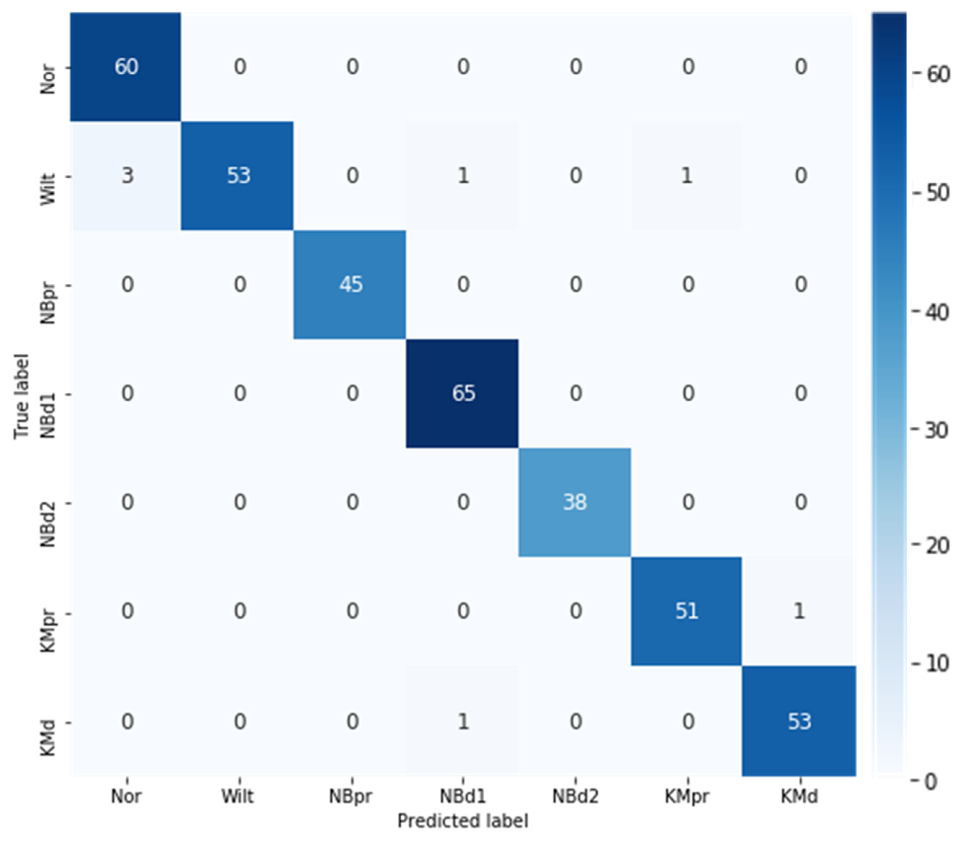
3.3. Best Model Performance Evaluation
4. Conclusions
Funding
Institutional Review Board Statement
Informed Consent Statement
Data Availability Statement
Acknowledgments
Conflicts of Interest
References
- Shah, D.; Tang, L.; Gai, J.; Putta-Venkata, R. Development of a mobile robotic phenotyping system for growth chamber-based studies of genotype x environment interactions. IFAC-PapersOnLine 2016, 49, 248–253. [Google Scholar] [CrossRef]
- Kim, Y.; Glenn, D.M.; Park, J.; Ngugi, H.K.; Lehman, B.L. Hyperspectral image analysis for water stress detection of apple trees. Comput. Electron. Agric. 2011, 77, 155–160. [Google Scholar] [CrossRef]
- Yang, M.; Cho, S.-I. High-Resolution 3D Crop Reconstruction and Automatic Analysis of Phenotyping Index Using Machine Learning. Agriculture 2021, 11, 1010. [Google Scholar] [CrossRef]
- Ge, Y.; Atefi, A.; Zhang, H.; Miao, C.; Ramamurthy, R.K.; Sigmon, B.; Yang, J.; Schnable, J.C. High-throughput analysis of leaf physiological and chemical traits with VIS–NIR–SWIR spectroscopy: A case study with a maize diversity panel. Plant Methods 2019, 15, 1–12. [Google Scholar] [CrossRef] [PubMed]
- Pandey, P.; Ge, Y.; Stoerger, V.; Schnable, J.C. High throughput in vivo analysis of plant leaf chemical properties using hyperspectral imaging. Front. Plant Sci. 2017, 8, 1348. [Google Scholar] [CrossRef] [PubMed]
- Nguyen, H.T.; Lee, B.-W. Assessment of rice leaf growth and nitrogen status by hyperspectral canopy reflectance and partial least square regression. Eur. J. Agron. 2006, 24, 349–356. [Google Scholar] [CrossRef]
- Elvanidi, A.; Katsoulas, N.; Ferentinos, K.; Bartzanas, T.; Kittas, C. Hyperspectral machine vision as a tool for water stress severity assessment in soilless tomato crop. Biosyst. Eng. 2018, 165, 25–35. [Google Scholar] [CrossRef]
- Sabatier, D.R.; Moon, C.M.; Mhora, T.T.; Rutherford, R.S.; Laing, M.D. Near-infrared reflectance (NIR) spectroscopy as a high-throughput screening tool for pest and disease resistance in a sugarcane breeding programme. Int. Sugar J. 2014, 116, 580–583. [Google Scholar]
- Li, F.; Mistele, B.; Hu, Y.; Chen, X.; Schmidhalter, U. Reflectance estimation of canopy nitrogen content in winter wheat using optimised hyperspectral spectral indices and partial least squares regression. Eur. J. Agron. 2014, 52, 198–209. [Google Scholar] [CrossRef]
- Shen, L.; Gao, M.; Yan, J.; Li, Z.-L.; Leng, P.; Yang, Q.; Duan, S.-B. Hyperspectral estimation of soil organic matter content using different spectral preprocessing techniques and PLSR method. Remote Sens. 2020, 12, 1206. [Google Scholar] [CrossRef]
- Zhou, X.; Sun, J.; Mao, H.; Wu, X.; Zhang, X.; Yang, N. Visualization research of moisture content in leaf lettuce leaves based on WT-PLSR and hyperspectral imaging technology. J. Food Process Eng. 2018, 41, e12647. [Google Scholar] [CrossRef]
- Muangprathub, J.; Boonnam, N.; Kajornkasirat, S.; Lekbangpong, N.; Wanichsombat, A.; Nillaor, P. IoT and agriculture data analysis for smart farm. Comput. Electron. Agric. 2019, 156, 467–474. [Google Scholar] [CrossRef]
- Wolfert, S.; Ge, L.; Verdouw, C.; Bogaardt, M.-J. Big data in smart farming—A review. Agric. Syst. 2017, 153, 69–80. [Google Scholar] [CrossRef]
- Rumpf, T.; Mahlein, A.-K.; Steiner, U.; Oerke, E.-C.; Dehne, H.-W.; Plümer, L. Early detection and classification of plant diseases with support vector machines based on hyperspectral reflectance. Comput. Electron. Agric. 2010, 74, 91–99. [Google Scholar] [CrossRef]
- Han, Q.; Li, Y.; Yu, L. Classification of glycyrrhiza seeds by near infrared hyperspectral imaging technology. In Proceedings of the 2019 International Conference on High Performance Big Data and Intelligent Systems (HPBD&IS), Shenzhen, China, 9–11 May 2019; pp. 141–145. [Google Scholar]
- Gbodjo, Y.J.E.; Ienco, D.; Leroux, L. Toward spatio–spectral analysis of sentinel-2 time series data for land cover mapping. IEEE Geosci. Remote Sens. Lett. 2019, 17, 307–311. [Google Scholar] [CrossRef]
- Masjedi, A.; Zhao, J.; Thompson, A.M.; Yang, K.-W.; Flatt, J.E.; Crawford, M.M.; Ebert, D.S.; Tuinstra, M.R.; Hammer, G.; Chapman, S. Sorghum biomass prediction using UAV-based remote sensing data and crop model simulation. In Proceedings of the IGARSS 2018—2018 IEEE International Geoscience and Remote Sensing Symposium, Valencia, Spain, 22–27 July 2018; pp. 7719–7722. [Google Scholar]
- Roscher, R.; Waske, B.; Forstner, W. Incremental import vector machines for classifying hyperspectral data. IEEE Trans. Geosci. Remote Sens. 2012, 50, 3463–3473. [Google Scholar] [CrossRef]
- Kamilaris, A.; Prenafeta-Boldú, F.X. Deep learning in agriculture: A survey. Comput. Electron. Agric. 2018, 147, 70–90. [Google Scholar] [CrossRef]
- Krizhevsky, A.; Sutskever, I.; Hinton, G.E. Imagenet classification with deep convolutional neural networks. Adv. Neural Inf. Processing Syst. 2012, 25, 1–9. [Google Scholar] [CrossRef]
- Han, Y.; Liu, Z.; Khoshelham, K.; Bai, S.H. Quality estimation of nuts using deep learning classification of hyperspectral imagery. Comput. Electron. Agric. 2021, 180, 105868. [Google Scholar] [CrossRef]
- Yang, W.; Yang, C.; Hao, Z.; Xie, C.; Li, M. Diagnosis of plant cold damage based on hyperspectral imaging and convolutional neural network. IEEE Access 2019, 7, 118239–118248. [Google Scholar] [CrossRef]
- Pérez-Pérez, B.D.; Garcia Vazquez, J.P.; Salomón-Torres, R. Evaluation of convolutional neural networks’ hyperparameters with transfer learning to determine sorting of ripe medjool dates. Agriculture 2021, 11, 115. [Google Scholar] [CrossRef]
- Saleem, M.H.; Potgieter, J.; Arif, K.M. Plant disease classification: A comparative evaluation of convolutional neural networks and deep learning optimizers. Plants 2020, 9, 1319. [Google Scholar] [CrossRef] [PubMed]
- Labhsetwar, S.R.; Haridas, S.; Panmand, R.; Deshpande, R.; Kolte, P.A.; Pati, S. Performance Analysis of Optimizers for Plant Disease Classification with Convolutional Neural Networks. In Proceedings of the 2021 4th Biennial International Conference on Nascent Technologies in Engineering (ICNTE), Navi Mumbai, India, 15–16 January 2021; pp. 1–6. [Google Scholar]
- Noon, S.K.; Amjad, M.; Qureshi, M.A.; Mannan, A. Overfitting mitigation analysis in deep learning models for plant leaf disease recognition. In Proceedings of the 2020 IEEE 23rd International Multitopic Conference (INMIC), Bahawalpur, Pakistan, 5–7 November 2020; pp. 1–5. [Google Scholar]
- Selvam, L.; Kavitha, P. Classification of ladies finger plant leaf using deep learning. J. Ambient. Intell. Humaniz. Comput. 2020, 1–9. [Google Scholar] [CrossRef]
- Dyrmann, M.; Karstoft, H.; Midtiby, H.S. Plant species classification using deep convolutional neural network. Biosyst. Eng. 2016, 151, 72–80. [Google Scholar] [CrossRef]
- Kussul, N.; Lavreniuk, M.; Skakun, S.; Shelestov, A. Deep learning classification of land cover and crop types using remote sensing data. IEEE Geosci. Remote Sens. Lett. 2017, 14, 778–782. [Google Scholar] [CrossRef]
- Garnot, V.S.F.; Landrieu, L.; Giordano, S.; Chehata, N. Time-space tradeoff in deep learning models for crop classification on satellite multi-spectral image time series. In Proceedings of the IGARSS 2019—2019 IEEE International Geoscience and Remote Sensing Symposium, Yokohama, Japan, 28 July–2 August 2019; pp. 6247–6250. [Google Scholar]
- Laban, N.; Abdellatif, B.; Ebeid, H.M.; Shedeed, H.A.; Tolba, M.F. Seasonal multi-temporal pixel based crop types and land cover classification for satellite images using convolutional neural networks. In Proceedings of the 2018 13th International Conference on Computer Engineering and Systems (ICCES), Cairo, Egypt, 18–19 December 2018; pp. 21–26. [Google Scholar]
- Li, Z.; Chen, G.; Zhang, T. A CNN-transformer hybrid approach for crop classification using multitemporal multisensor images. IEEE J. Sel. Top. Appl. Earth Obs. Remote Sens. 2020, 13, 847–858. [Google Scholar] [CrossRef]
- Zhang, N.; Yang, G.; Pan, Y.; Yang, X.; Chen, L.; Zhao, C. A review of advanced technologies and development for hyperspectral-based plant disease detection in the past three decades. Remote Sens. 2020, 12, 3188. [Google Scholar] [CrossRef]
- Ariana, D.P.; Lu, R.; Guyer, D.E. Near-infrared hyperspectral reflectance imaging for detection of bruises on pickling cucumbers. Comput. Electron. Agric. 2006, 53, 60–70. [Google Scholar] [CrossRef]
- Sarasketa, A.; González-Moro, M.B.; González-Murua, C.; Marino, D. Nitrogen source and external medium pH interaction differentially affects root and shoot metabolism in Arabidopsis. Front. Plant Sci. 2016, 7, 29. [Google Scholar] [CrossRef]
- Nestby, R.; Lieten, F.; Pivot, D.; Lacroix, C.R.; Tagliavini, M. Influence of mineral nutrients on strawberry fruit quality and their accumulation in plant organs: A review. Int. J. Fruit Sci. 2005, 5, 139–156. [Google Scholar] [CrossRef]
- Wang, J.; Liu, X.; Huang, F.; Tang, J.; Zhao, L. Salinity forecasting of saline soil based on ANN and hyperspectral remote sensing. Trans. Chin. Soc. Agric. Eng. 2009, 25, 161–166. [Google Scholar]
- Grinblat, G.L.; Uzal, L.C.; Larese, M.G.; Granitto, P.M. Deep learning for plant identification using vein morphological patterns. Comput. Electron. Agric. 2016, 127, 418–424. [Google Scholar] [CrossRef] [Green Version]
- Karpathy, A. Convolutional Neural Networks. Available online: http://cs231n.github.io/convolutional-networks (accessed on 18 September 2022).
- Polyak, B.T. Some methods of speeding up the convergence of iteration methods. USSR Comput. Math. Math. Phys. 1964, 4, 1–17. [Google Scholar] [CrossRef]
- Duchi, J.; Hazan, E.; Singer, Y. Adaptive subgradient methods for online learning and stochastic optimization. J. Mach. Learn. Res. 2011, 12, 2121–2159. [Google Scholar]
- Ruder, S. An overview of gradient descent optimization algorithms. arXiv 2016, arXiv:1609.04747. [Google Scholar]
- Jiang, Q.; Wu, G.; Tian, C.; Li, N.; Yang, H.; Bai, Y.; Zhang, B. Hyperspectral imaging for early identification of strawberry leaves diseases with machine learning and spectral fingerprint features. Infrared Phys. Technol. 2021, 118, 103898. [Google Scholar] [CrossRef]


| Symptom | Class Abbr. | Training | Validation | Test | Total |
|---|---|---|---|---|---|
| Normal | Nor | 404 | 120 | 60 | 584 |
| Wilt | Wilt | 390 | 104 | 58 | 552 |
| N, B deficiency prediction | NBpr | 329 | 98 | 45 | 472 |
| N, B deficiency Stage 1 | NBd1 | 438 | 121 | 65 | 624 |
| N, B deficiency Stage 2 | NBd2 | 289 | 73 | 38 | 400 |
| K, Mg deficiency prediction | KMpr | 311 | 85 | 52 | 448 |
| K, Mg deficiency | KMd | 453 | 133 | 54 | 640 |
| Total | 2614 | 734 | 372 | 3720 | |
| Optimizer | Time (s) | Epochs | s/Epoch | Accuracy | ||
|---|---|---|---|---|---|---|
| Train | Validation | Test | ||||
| SGD | 6794.2 | 10,000 | 0.679 | 0.169 | 0.1761 | 0.145 |
| Adagrad | 1509.2 | 2246 | 0.672 | 0.935 | 0.918 | 0.933 |
| RMSProp | 513.4 | 753 | 0.682 | 0.951 | 0.957 | 0.957 |
| Adam | 724.7 | 1075 | 0.674 | 0.982 | 0.978 | 0.981 |
| Class (Abbr.) | Precision | Recall | F1 Score |
|---|---|---|---|
| Normal (Nor) | 0.95 | 1.00 | 0.98 |
| Wilt (Wilt) | 1.00 | 0.91 | 0.95 |
| N, B deficiency prediction (NBpr) | 1.00 | 1.00 | 1.00 |
| N, B deficiency Stage 1 (NBd1) | 0.97 | 1.00 | 0.98 |
| N, B deficiency Stage 2 (NBd2) | 1.00 | 1.00 | 1.00 |
| K, Mg deficiency prediction (KMpr) | 0.98 | 0.98 | 0.98 |
| K, Mg deficiency (KMd) | 0.98 | 0.98 | 0.98 |
| Macro avg. | 0.98 | 0.98 | 0.98 |
| Weighted avg. | 0.98 | 0.98 | 0.98 |
Publisher’s Note: MDPI stays neutral with regard to jurisdictional claims in published maps and institutional affiliations. |
© 2022 by the author. Licensee MDPI, Basel, Switzerland. This article is an open access article distributed under the terms and conditions of the Creative Commons Attribution (CC BY) license (https://creativecommons.org/licenses/by/4.0/).
Share and Cite
Yang, M. Physiological Disorder Diagnosis of Plant Leaves Based on Full-Spectrum Hyperspectral Images with Convolutional Neural Network. Horticulturae 2022, 8, 854. https://doi.org/10.3390/horticulturae8090854
Yang M. Physiological Disorder Diagnosis of Plant Leaves Based on Full-Spectrum Hyperspectral Images with Convolutional Neural Network. Horticulturae. 2022; 8(9):854. https://doi.org/10.3390/horticulturae8090854
Chicago/Turabian StyleYang, Myongkyoon. 2022. "Physiological Disorder Diagnosis of Plant Leaves Based on Full-Spectrum Hyperspectral Images with Convolutional Neural Network" Horticulturae 8, no. 9: 854. https://doi.org/10.3390/horticulturae8090854