Article

SwinGD: A Robust Grape Bunch Detection Model Based on Swin Transformer in Complex Vineyard Environment

1
College of Electronic and Information Engineering, Foshan University, Foshan 528000, China
2
College of Mechanical and Electrical Engineering, Foshan University, Foshan 528000, China
*
Author to whom correspondence should be addressed.
Horticulturae 2021, 7(11), 492; https://doi.org/10.3390/horticulturae7110492
Submission received: 6 October 2021 / Revised: 7 November 2021 / Accepted: 10 November 2021 / Published: 12 November 2021

Abstract

:
Accurate recognition of fruits in the orchard is an important step for robot picking in the natural environment, since many CNN models have a low recognition rate when dealing with irregularly shaped and very dense fruits, such as a grape bunch. It is a new trend to use a transformer structure and apply it to a computer vision domain for image processing. This paper provides Swin Transformer and DETR models to achieve grape bunch detection. Additionally, they are compared with traditional CNN models, such as Faster-RCNN, SSD, and YOLO. In addition, the optimal number of stages for a Swin Transformer through experiments is selected. Furthermore, the latest YOLOX model is also used to make a comparison with the Swin Transformer, and the experimental results show that YOLOX has higher accuracy and better detection effect. The above models are trained under red grape datasets collected under natural light. In addition, the dataset is expanded through image data augmentation to achieve a better training effect. After 200 epochs of training, SwinGD obtained an exciting mAP value of 94% when IoU = 0.5. In case of overexposure, overdarkness, and occlusion, SwinGD can recognize more accurately and robustly compared with other models. At the same time, SwinGD still has a better effect when dealing with dense grape bunches. Furthermore, 100 pictures of grapes containing 655 grape bunches are downloaded from Baidu pictures to detect the effect. The Swin Transformer has an accuracy of 91.5%. In order to verify the universality of SwinGD, we conducted a test under green grape images. The experimental results show that SwinGD has a good effect in practical application. The success of SwinGD provides a new solution for precision harvesting in agriculture.

1. Introduction

In recent years, China’s grape production increased year by year. As of 2014, China’s grape planting area has reached 767.2 thousand hectares (7672 km2), and the output has become the first in the world [1]. Grape harvesting is a time-consuming and labor-intensive procedure [2,3]. However, with the aging of the population and the decrease in labor force due to fewer young and middle-aged people in China, the timely harvesting of fruits is becoming a significant challenge for fruit growers. Driven by the wave of artificial intelligence, the intelligent management of orchards is imperative [4]. Among them, the automatic identification and detection of fruits is an important prerequisite for intelligent planting and picking [5,6]. In the natural environment, the detection of grapes in orchards has problems, such as leaves, mutual blocking of grapes, and uneven light irradiation, making manual conventional detection methods for feature extraction difficult for accurate detection. Therefore, it is very necessary to develop an automatic grape harvesting system. For automatic harvesting, the major task is to detect and locate grape bunches in a vineyard by using artificial vision.
To design strategies to improve picking efficiency, it is important to examine the use of intelligent robots for harvesting fruits. For the past 30 years, scholars from different parts of the world have studied fruit-harvesting robots, including harvesting robots for strawberry [7], cucumber [8], apple [9], sweet pepper [10], citrus [11], litchi [12,13], banana [14], mango [15], and so on. However, up to now, commercial automatic harvesting robots are still rarely reported, and one of the main reasons is low location accuracy in unstructured orchards. To realize practical robotics harvesting, the minimum accuracy required for real harvesting systems is more than 80%.
With artificial intelligence developing, deep learning is widely used for image recognition. All kinds of neural networks and deep learning models have emerged [16,17,18]. However, harvesting of fruits requires higher real-time performance. In order to be able to start faster, real-time sensing is important, which requires a model that can detect objects in near real time. The most popular real-time framework detection frameworks are Faster-RCNN, YOLO, and SSD [19,20,21]. Faster-RCNN shows higher accuracy in benchmark tests, but YOLO can infer prediction results faster. In this paper, two YOLO models are included: one is the latest YOLOX [22], and the other is the classic YOLOV3-SPP [23,24]. Furthermore, the transformer structure has achieved the most advanced results for many natural language processing tasks [25,26,27]. In the field of computer vision, CNN has been the dominant model for visual tasks [28,29,30] since 2012. With the emergence of more and more efficient structures, and the convergence of computer vision and natural language processing, the use of a transformer to complete visual tasks [31,32] has become a new research direction to reduce the complexity of structures and explore scalability and training efficiency. By limiting the self-attention calculation to nonoverlapping local windows, while allowing cross-window connections, the shifted window scheme brings greater efficiency. A Swin Transformer is an innovative vision model of a transformer [33,34,35] that demonstrates powerful capabilities for image processing. This hierarchical architecture has the flexibility to model at a variety of scales and has linear computational complexity relative to image size. These qualities of the Swin Transformer make it compatible with a variety of visual tasks. In order to compare with the performance of models for grape detection, in this paper, models of SSD, DETR [36], Faster-RCNN, YOLOX, and YOLOv3-SPP are proposed to make a comparison in the augmentation dataset. The experimental results show that the advantages of the Swin Transformer is that it is better in grape detection.

2. Materials and Methods

2.1. Architecture Overview

Recently, a transformer [37] model for natural language processing has gained much popularity in computer vision, when used in vision problems, such as object detection, image classification, segmentation, and crowd counting. It learns to attend to important image regions by exploring the global interactions between different regions. Due to its impressive performance, the transformer has also been introduced for intelligent agriculture.
The Swin Transformer is a pure transformer architecture model and becoming a general-purpose backbone for various vision tasks, especially Swin-L as a backbone in HTC++ [38] frameworks. This model achieves 58.7 box AP that creates a new record in the object detection domain. The Swin Transformer imitates the CNN’s hierarchical architecture. In the initialization phase, the images are cut up into small-size patches and gradually merging neighboring patches in deeper transformer layers, as shown in Figure 1a. The computational complexity goes from quadratic to linear by computing self-attention using the nonoverlapping windows. However, this division would decrease the connection of each window. Facing this problem, the model takes up the shifted window approach to solve it. The shifted windows are shown in Figure 1b. The shifted windows contribute to the connection of each window of the preceding layer, which significantly enhances the modeling effect. In this way, the disadvantages of the missing global effect are overcome. At the same time, this is the main difference from the original transformer architecture.
An overall architecture of the Swin Transformer is shown in Figure 2. At first, the grape images are split into nonoverlapping patches with a patch size of 4 × 4. Thus the feature dimension of each patch is 4 × 4 × 3. Furthermore, a linear embedding layer is applied to the projected feature dimension into an arbitrary dimension (represented as C). The transformed patch tokens pass through several Swin Transformer blocks and patch merging layers to generate the hierarchical feature representations. Specifically, the patch merging layer is responsible for downsampling and increasing the dimension, and a Swin Transformer block is responsible for feature representation learning.
As illustrated in Figure 3, it can be seen that multiheaded self-attention (MSA) is constructed based on shift windows. There are two consecutive Swin Transformer blocks. Each Swin Transformer block is composed of a LayerNorm (LN) layer, multihead self-attention module, residual connection, and multilayer perceptron (MLP) that has two fully connected layers with GELU nonlinearity. The window-based multihead self-attention (W-MSA) module and the shifted window-based multihead self-attention (SW-MSA) module are applied in the two successive transformer blocks, respectively. Based on such window partitioning mechanism, continuous Swin Transformer blocks can be formulated as:
z ^ l = W M S A ( L N ( z l 1 ) ) + z l 1
z l = M L P ( L N ( z ^ l ) ) + z ^ l
z ^ l + 1 = S W M S A ( L N ( z l ) ) + z l
z l + 1 = M L P ( L N ( z ^ l + 1 ) ) + z ^ l + 1
where z ^ l and z l represent the outputs of the (S)W-MSA module and the MLP module of the l t h block, respectively.
Similar to previous works [39,40], given an input of size, H × W × C , the Swin Transformer first reshapes the input to a H W M 2 × M 2 × C feature. Additionally, a window contains M × M patches, and the total number of windows is H W M 2 . Then, self-attention is calculated for each patch. For a patch feature, X M 2 × C , the query, key, and value matrices, Q , K and V , are computed as
Q = X P Q , K = X P K , V = X P V
where P Q , P K , and P V are projection matrices that are shared across different windows. Self-attention is computed as follows:
Attention ( Q , K , V ) = SoftMax ( Q K T d + B ) V
where Q , K , V M 2 × d , and d represent the dimension of the query or key. Additionally, the values in B are taken from the bias matrix B ^ ( 2 M 1 ) × ( 2 M + 1 ) . In this way, the computation complexity gets a huge optimization.

2.2. Training

The collected images were assigned a training set and a validation set with a probability of 6 to 1. In addition, in order to avoid overfitting, the image augmentation was used and is mentioned in the above section.
The experiments were performed on a custom red grape dataset. In the following, the advantages and disadvantages of the Swin Transformer, DETR, YOLOv3-SPP, Faster-RCNN, YOLOX, and SSD are compared in terms of object detection. The initialization parameters, such as initial learning rate, weight decay regularization, and batch size, of these models are shown in Table 1.
The above models adopted a PyTorch-based implementation. The pretraining weights were trained previously on a COCO 2017 dataset. These models were trained in a computer containing a single GPU of GeForce RTX 2080Ti, 11 GB memory (NVIDIA Corporation, Santa Clara, CA, USA) and a CPU of i5-7400 (Intel corporation, Santa Clara, CA, USA) and 64 GB RAM. It ran under the Ubuntu 18.04 LTS operating system. For training time at 200 epochs, the Swin Transformer model took 3 h to train the red grape dataset, the YOLOv3-SPP model spent 4 h and 10 min, the SSD model spent 45 min, and Faster-RCNN spent 8 h and 50 min. For the DETR model, training was performed in approximately 3 h and 40 min. However, YOLOX’s training time was 9 h and 40 min.

2.3. Evaluation

In this article, the mAP value is used as evaluation metrics. The mAP value measurements depend on the following indicators. The meanings and calculation methods of relevant indicators are as follows:
  • Intersection over union (IoU) is a radio of overlaps between the ground truth and the prediction bounding box in the dataset. The detail is shown in Formula (7):
I o U = A B A B
  • True positive (TP) refers to the number of detection boxes that are capable of expression objects. In this paper, the object refers to the red grapes. IoU > 0.5 in the ground truth and prediction bounding box that the bounding box is truly positive.
  • False positive (FP) refers to the number of detection boxes in which IoU < 0.5. It shows that the prediction bounding box is not performed well in the object.
  • False negative (FN) refers to the number of prediction bounding boxes that are not in the ground truth.
  • Precision (P) refers to the ratio of the true prediction bounding boxes in all prediction bounding boxes. The detail is shown in Formula (8):
P = T P T P + F P
  • Recall (R) refers to the radio of the true bounding boxes in all ground truths. The detail is shown in Formula (9):
R = T P T P + F N
The precision–recall (PR) curve can be obtained by using the recall ratio as the horizontal axis and the precision ratio as the vertical axis. The mAP (mean average precision) value is used to evaluate the performance of the model. Additionally, the AP (average precision) is an integral of the PR curve over the recall rate based on accuracy, and the mAP value represents the average AP value of multiple objects, which is a standard for measuring the precision of the network to target objects. A higher AP value represents higher identification accuracy.

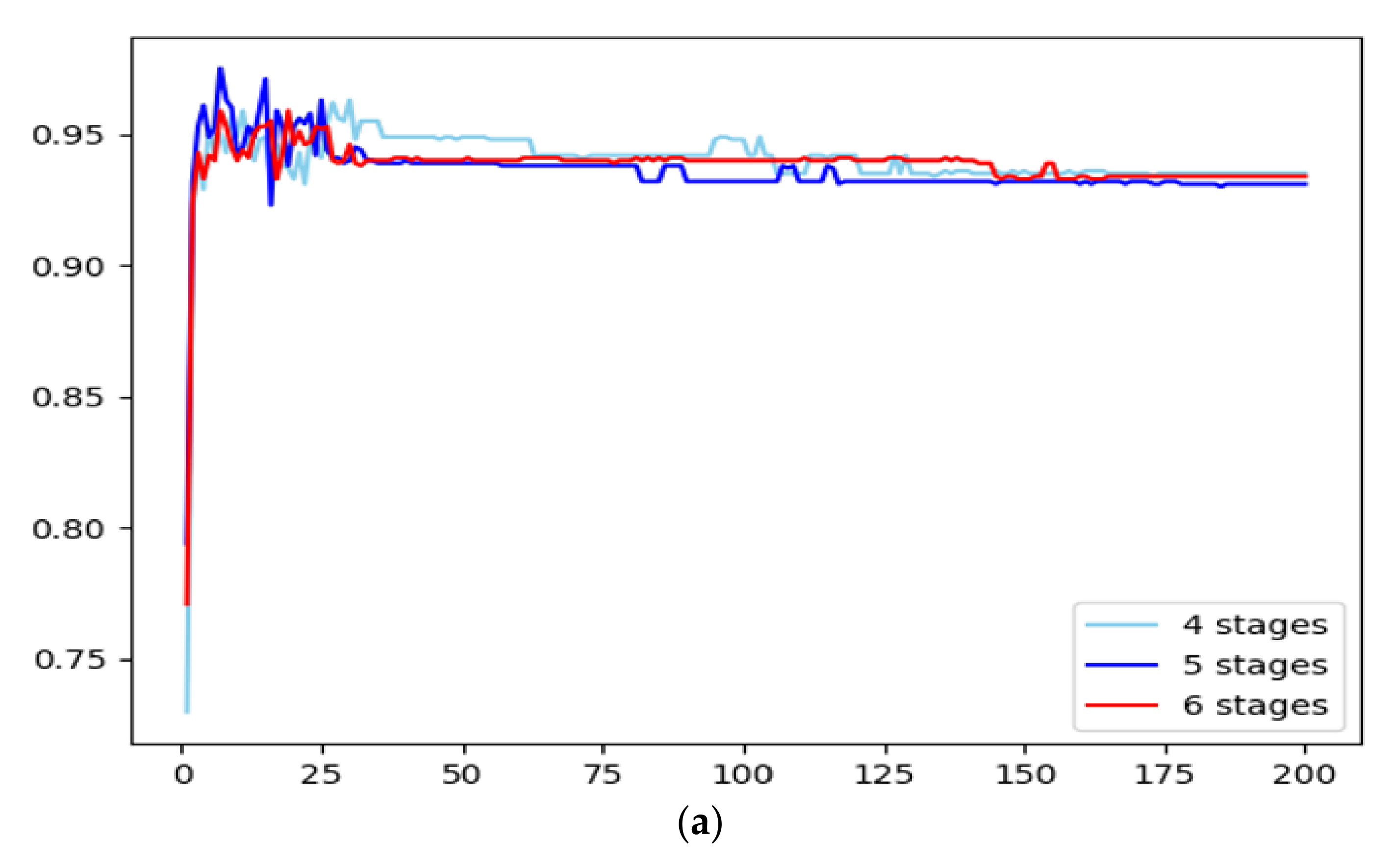
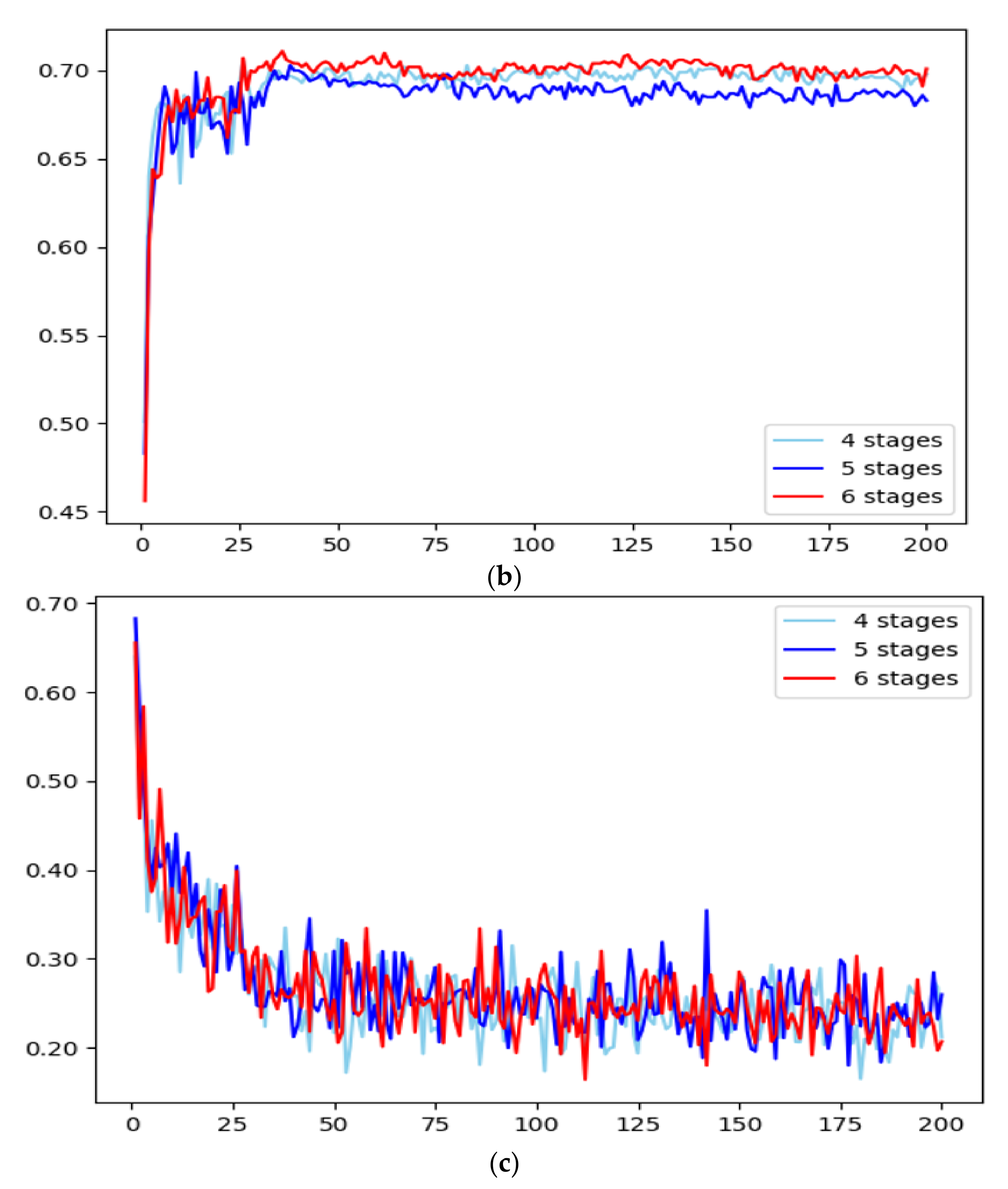
2.4. Swin Transformer Architecture with Different Stages

In this section, the standard Swin Transformer structure was changed to further explore the impact of layers on detection results. As shown in Figure 4, Figure 4a,b is equivalent to adding one and two stages to Figure 2, respectively. The above three models were trained in the same training set. The training set has 606 images, and the validation set has 101 images. The specific experimental results are shown in Figure 5. As shown in Figure 5a, the three Swin Transformer models with different stages present a similar mAP value of about 94% in the case of IoU = 0.5. In addition to the above evaluation index, another mAP value can be obtained when IoU = 0.50:0.05:0.95. It is the most important index to evaluate the performance of the model in the COCO 2017 dataset. IoU = 0.5:0.05:0.95 means that from IoU = 0.5, the value begins to increase at a growth rate of 0.05 until it reaches IoU = 0.95. As shown in Figure 5b, the Swin Transformer with six stages has the best performance, and the Swin Transformer with five stages has the worst performance, whose mAP values are 70% and 68%, respectively. Additionally, the training loss values of the three models have a similar performance in Figure 5c. It can be explained that more stages of the Swin Transformer do not mean better efficiency. Therefore, the Swin Transformer with four stages is adopted to achieve the desired detection effect. In the next section, the Swin Transformer with four stages is used to make a comparison with other models.

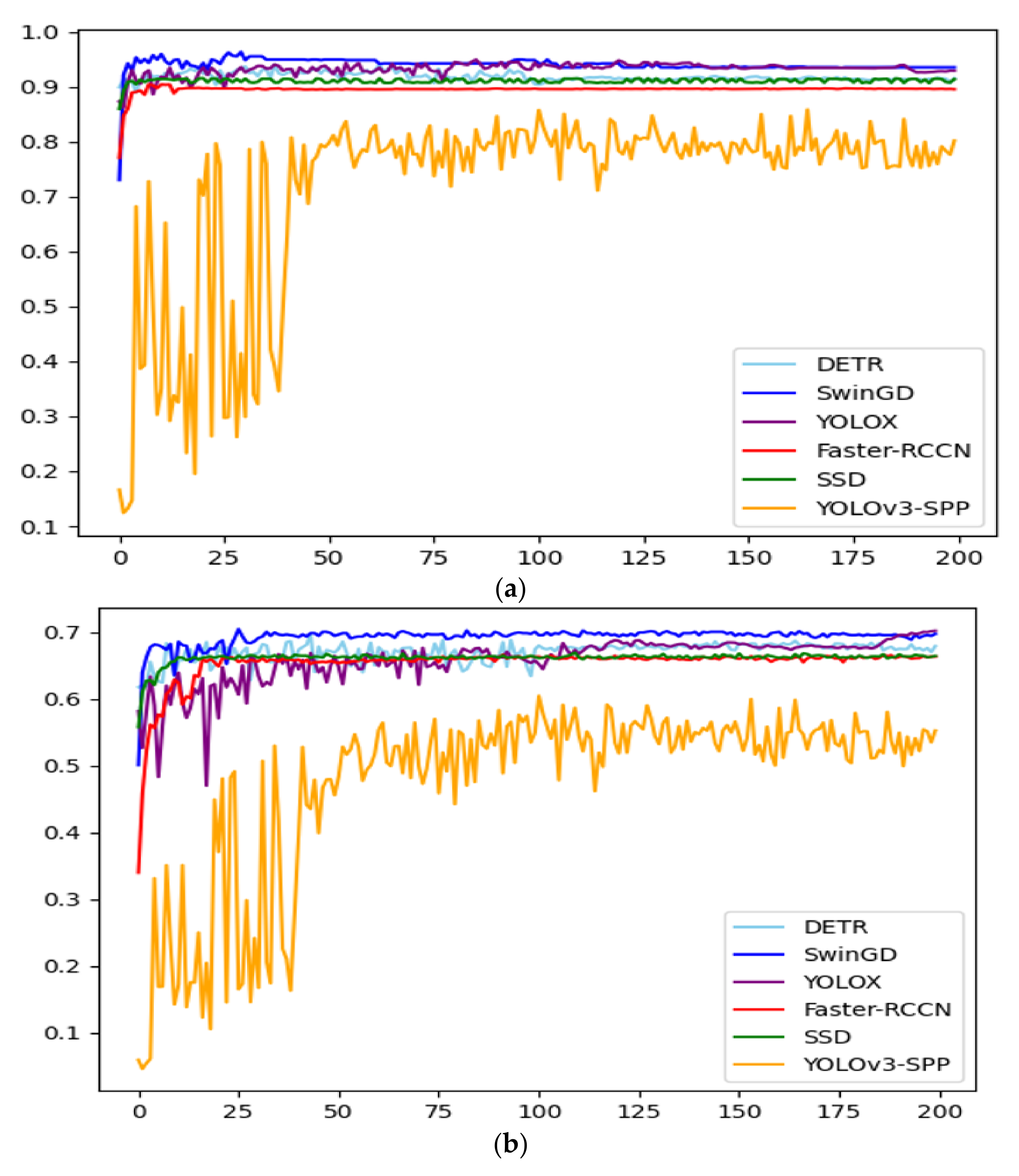
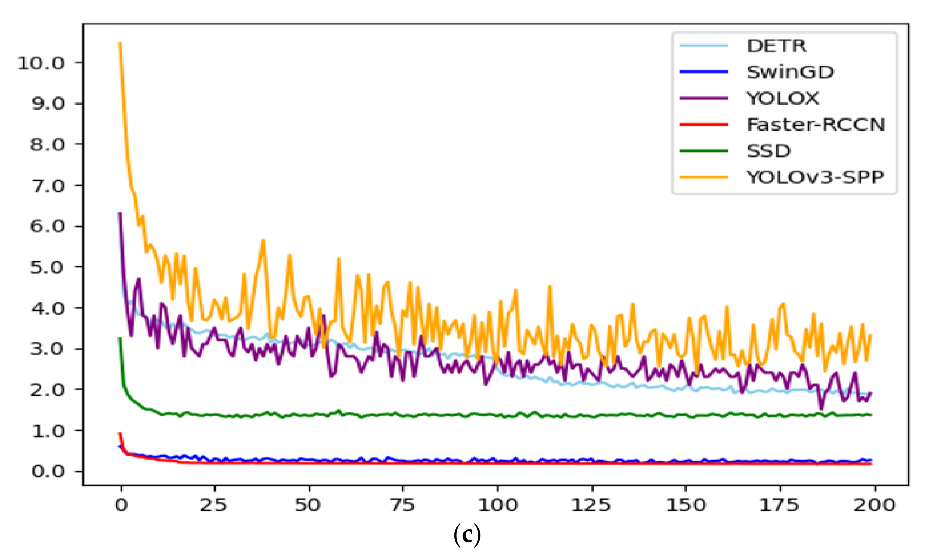
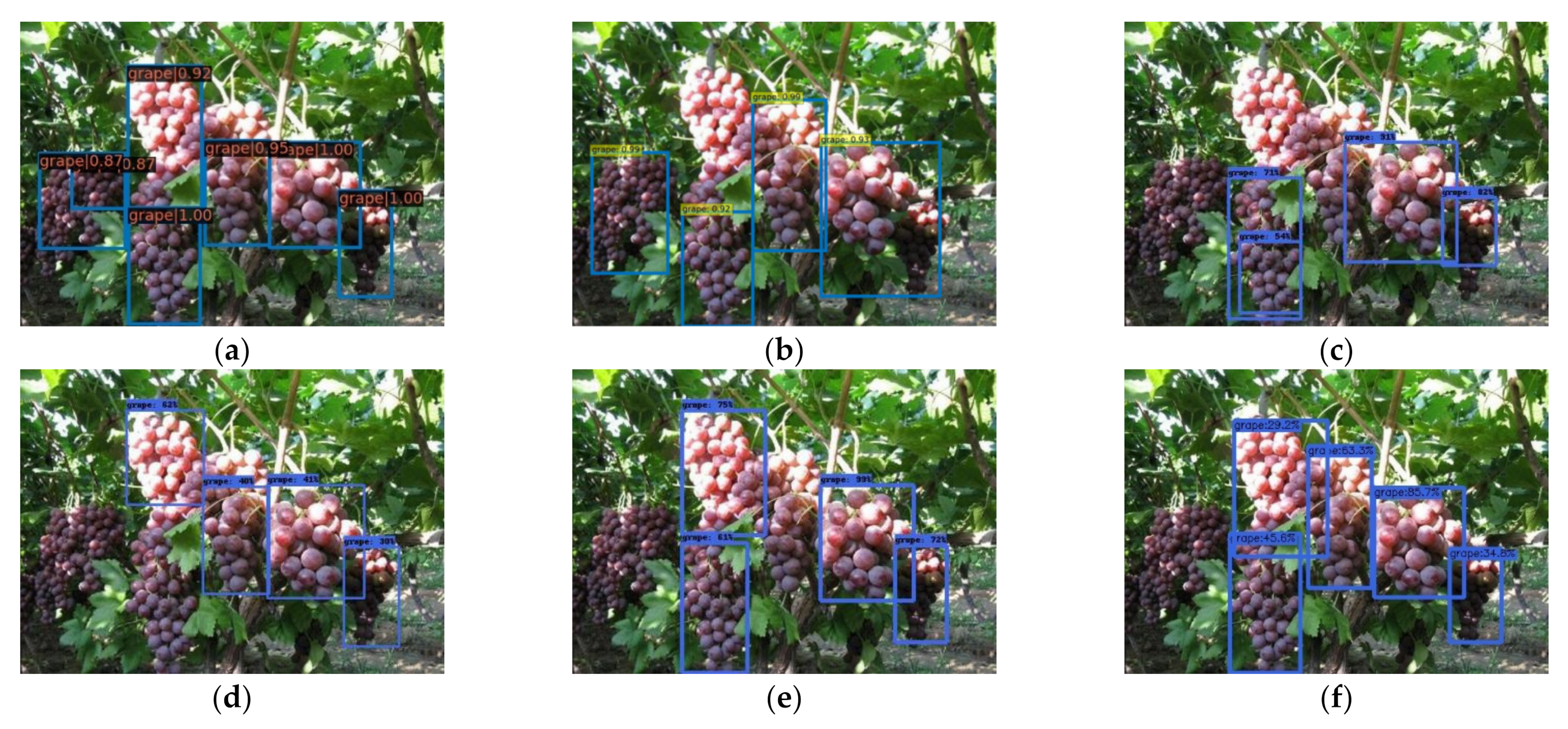
2.5. Comparison of Different Models

In order to verify the performance of SwinGD, the models, including SSD, DETR, Faster-RCNN, YOLOX, and YOLOv3-SPP, are proposed to make a comparison in the augmentation dataset.
The grape dataset was trained on different models, and the training results of each model were recorded. At first, the mAP value with IoU = 0.5 was considered. For example, as shown in Figure 6a, SwinGD with a blue curve has a better mAP score above 94%. Especially, the mAP value of SwinGD could reach 95% in the early epochs and kept a stable objection detection result in the latter epochs. The experiment expresses that SwinGD does not need too many epochs, and it is enough for us to train 36 epochs to get a better result. On the contrary, the DETR model with a sky blue curve in Figure 6a is not stable at the early epochs, and the mAP value reaches 91% in the end. The reason why DETR is much less effective than SwinGD is that DETR needs enough epochs to get a good result. However, YOLOX with a brown curve in Figure 6a has an impressive performance. After 80 epochs, the mAP values of SwinGD and YOLOX tend to consistently achieve 94% accuracy. Compared with SwinGD, YOLOX achieves similar accuracy but is less stable and fluctuates greatly. The SSD model with a green curve in Figure 6a is also worse than SwinGD, but it keeps a stable mAP value of around 91%. Additionally, the mAP value remains similar to that of DETR. As we all know, grape bunches are very vulnerable to damage; therefore, a higher value of accuracy is required in the identification process. Faster-RCNN with a red curve in Figure 6a has worse accuracy than SSD, but it keeps an extremely stable algorithm than SSD. Additionally, the accuracy rates fluctuate at around 89%. As for the YOLOv3-SPP model with an orange curve, it has an unstable effect on grape bunch detection in the beginning epochs. Even at the best epoch, it only has an accuracy of 80%. As illustrated in Figure 6a, SwinGD has the best training result among the above models.
As shown in Figure 6b, it is more obvious that SwinGD has the best effect in the case of IoU = 0.50:0.05:0.95. More specifically, SwinGD with a blue curve has a good convergence effect and keeps a value of mAP of around 70%. The DETR model with a sky blue curve has a value of about 68%, which is significantly lower than that of SwinGD. At the same time, the mAP value of YOLOX with a brown curve is significantly lower than that of SwinGD and DETR models. This indicates that YOLOX’s overall performance is not very good. The SSD model with a green curve and the Faster-RCNN model with a red curve have a stable convergence and reach 66% and 65%, respectively. Compared with other methods, the YOLOv3-SPP model with an orange curve has the worst mAP value of below 60%.
The training loss image of each model is shown in Figure 6c. SwinGD has a low loss value between 0.2 and 0.3. Additionally, Faster-RCNN also has a similar loss value of about 0.2. The DETR, SSD, YOLOX, and YOLOv3-SPP models have a value of 2, 1.35, 2, and 3, respectively. The above three models have significantly higher loss values than SwinGD and Faster-RCNN. By comparing the loss values of each model above, the superiority of SwinGD is further proved.
The training loss image of each model is shown in Figure 6c. SwinGD has a low loss value between 0.2 and 0.3. Additionally, Faster-RCNN also has a similar loss value of about 0.2. The DETR, SSD, YOLOX, and YOLOv3-SPP models have values of 2, 1.35, 2, and 3, respectively. The above three models have significantly higher loss values than SwinGD and Faster-RCNN. By comparing the loss values of each model above, the superiority of SwinGD is further proved.
It can be seen from the above three experimental results that SwinGD has the best results and is the most suitable for grape bunch detection.

3. Results

3.1. Image Dataset

The grape dataset are red grapes in this paper, captured during daylight hours at an orchard in Foshan. Datasets are composed of 200 RGB images. In order to satisfy the need for grape detection, the software of LabelImg is used in the ubuntu18.04 to mark pictures. The software allows users to mark the object of interest using rectangles, circles, and polygons. In this paper, the rectangles are used to mark red grapes. Additionally, the software will produce an XML file that includes label and position information. The XML files are the format of the PASCALL-VOC [41] datasets. The datasets are split into two parts: one is the training set, and the other is the validation set. In the next section, the data augmentation is used to expand the number of images. The training set has 606 images, and the validation set has 101 images. Additionally, the maximum number of iterations is set to 200. In addition, the program is executed to convert PASCALL-VOC format to COCO 2017 [42] format and YOLO format. Finally, the test sets are collected in Baidu images.

3.2. Image Data Augmentation

The common method for enhancing the image dataset is to use geometric transformations and color transformations. Using these methods, the richness of the experimental dataset are obtained. These pictures were preprocessed about rotation, flap, brightness, and color. The human visual system could detect the same objects under different lighting and external conditions, but the imaging device has a hard time recognizing in the same circumstance. That is why models need to be trained on large datasets. In this way, the model is more robust in the face of complex environments.

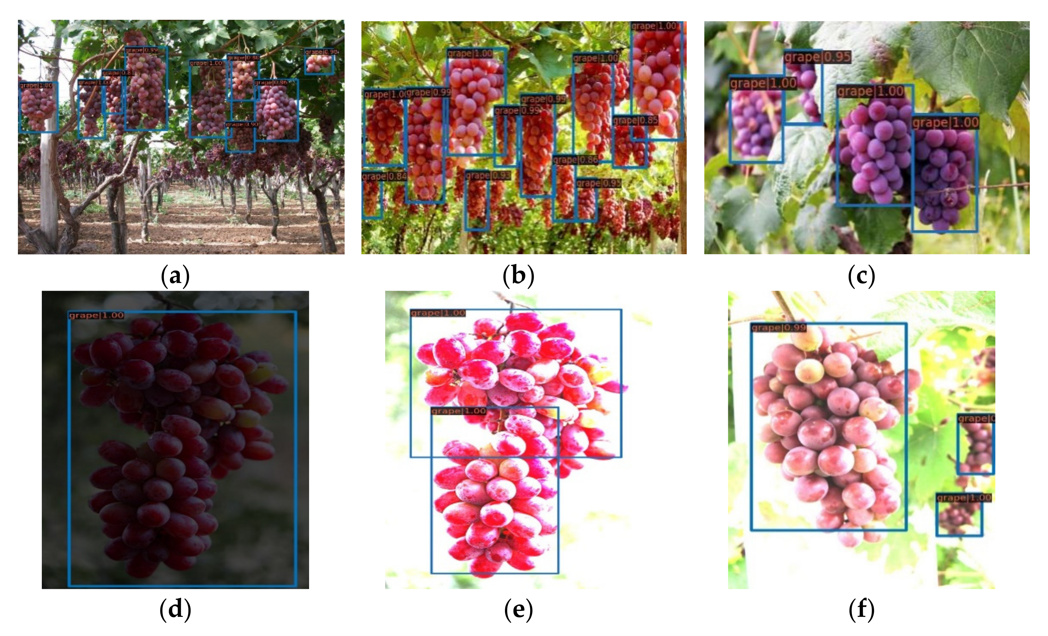
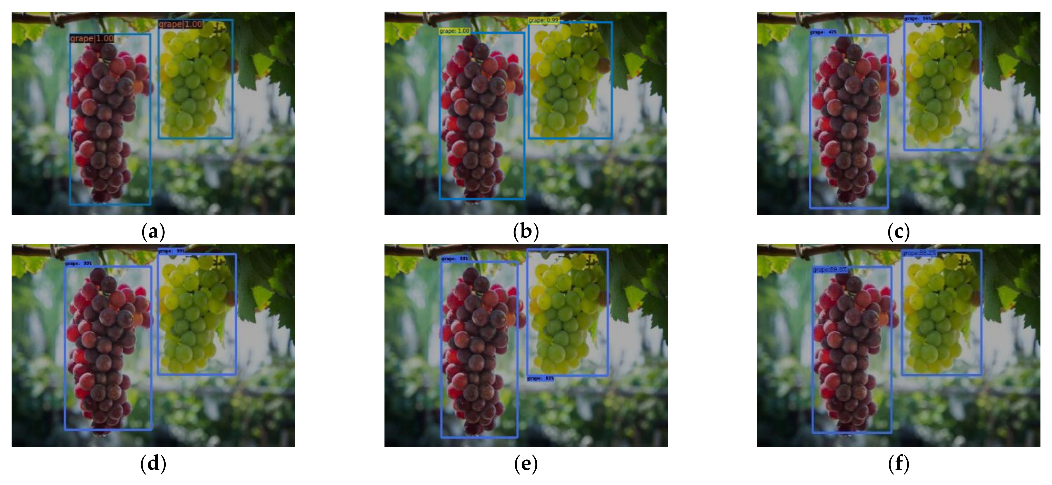
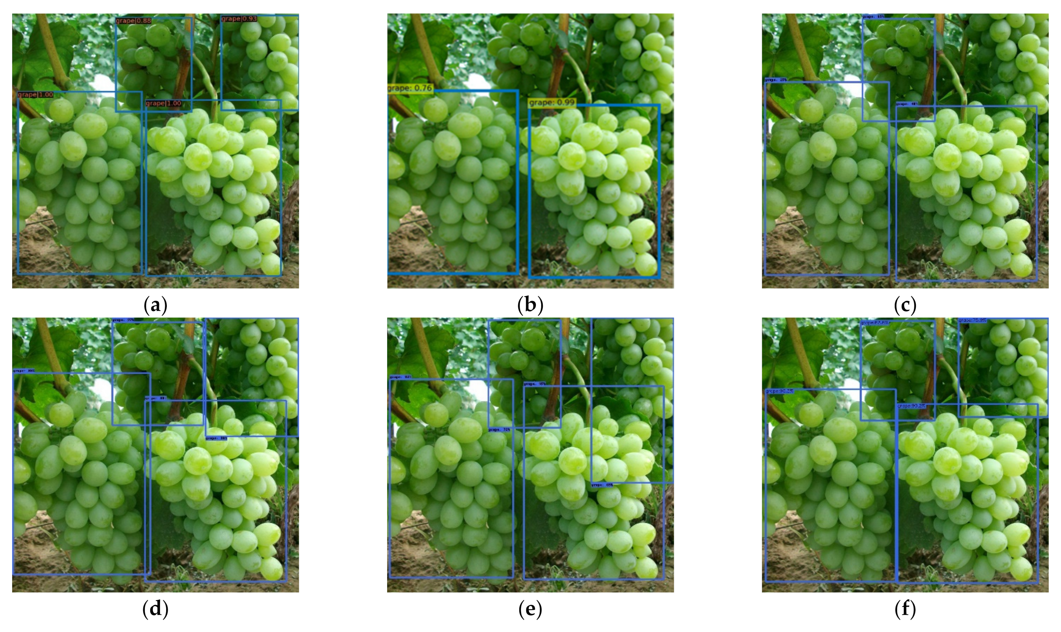
3.3. The Effect of SwinGD in Different Cases

Putting the above trained models to predict the test set, the detection effect of various models in different environments can be further judged in this section. Under the natural environment, fruit detection will meet a variety of complex situations. It will produce a serious impact on the effect of detection. Next, the effect of the external environment on SwinGD detection is shown. As shown in Figure 7, SwinGD has a better effect on grape bunches detection under different circumstances. For example, when there are many grape bunches in one picture, just like in Figure 7a–c, most of the grape bunches are recognized by SwinGD. Even in an overexposed or underdark environment, SwinGD can also have a good effect, just like in Figure 7d–f. In the following sections, SwinGD is used to make a comparison with other models in the same grape dataset.

3.4. Detection Effect of Dense Grape Bunches and Dark Environment

In some situations, the dense bunches of grapes need to be identified. As shown in Figure 8, SwinGD, DETR, and YOLOX have a better detection effect than the rest of the models. SwinGD could detect all the grape bunches, and DETR and YOLOX have one grape left undetected. On the contrary, the remaining models had a bad performance and only a fraction of the grape bunches were detected.
Poor external conditions are often encountered during grape bunch picking. For instance, dim weather is a common problem encountered. In practice, the picking robot used by our team adopts an ordinary RGB camera rather than an infrared camera, which requires too much light, so it cannot detect grape bunches well in a dark environment. As shown in Figure 9, each model can identify grape bunches in dark environments. In some relatively simple environments, SwinGD has similar performance to other models. This shows that the slightly dark environment does not affect the detection effect of each algorithm.

3.5. The Applicability of SwinGD

Furthermore, the applicability of these models to different grape varieties will be discussed. In real life, there are many green grapes besides red grapes in vineyards. In Figure 10, the results of the recognition of green grape bunches by different models are presented. As shown in Figure 10a,d–f, SwinGD, Faster-RCNN, SSD, and YOLOX had a good performance in which all grape bunches were identified. SwinGD and YOLOX still retained the best detection effect in that the size and position of the grape bunches were accurately identified. Besides, YOLOv3-SPP and DETR still had one grape bunch and two grape bunches that were not detected, respectively, as shown in Figure 10b,c.
As you can see from Figure 11a,f, both SwinGD and YOLOX have excellent robustness. SwinGD and YOLOX not only recognizes all green grape bunches but also distinguishes two bunches of similar grape bunches. However, the confidence values of YOLOX is lower than those of SwinGD. On the contrary, as shown in Figure 11b–d the DETR, Faster-RCNN, and YOLOv3-SPP models cannot distinguish particularly similar grape bunches. The SSD model had an obviously bad effect compared with the above models in that only three bunches of grapes were detected, as shown in Figure 11e.
More details are observed in Figure 12. SwinGD can detect small bunches of grapes that look similar to the background and further demonstrated the ability to identify grape bunches. YOLOX and YOLOv3-SPP detected two out of three bunches of grapes, but there was an incorrect detection. In the face of complex background conditions, Faster-RCNN and SSD are only ones able to detect the largest bunch in the middle of the picture. Compared with other CNN-based models in the paper, the DETR model also presents a better detection effect.
None of the above models were trained with a green grape dataset. The results from the above three pictures indicate that SwinGD shows the best detection results compared with the other models. The YOLOX model also presents a stable and better result compared with the other models in most instances.

3.6. Experiment Result in Different Grape Test Sets

Additionally, an extra dataset was used to evaluate the actual detection effect. The red grape test set and the green grape test set each had 100 images. They were all collected from Baidu images. The numbers of grape bunches in the red dataset and the green dataset were 655 and 360 images, respectively. The detection accuracy of various models is shown in Table 2.
On the one hand, some models did not show good performance for the red grape test results. That is because some small grape bunches were not detected in the image. All the models were not trained to detect the small grape bunches in the training set. However, SwinGD, YOLOX, and DETR could detect the small grape bunches in the same circumstance. Faster-RCNN, SSD, and YOLOv3-SPP had a good effect on the big grape bunches. As for the results of the green grape bunches test, SwinGD also had a better result than other models. According to the detection results, SwinGD has a higher applicability and is more suitable for facing various complex environments.
Finally, the inference time of five models was compared. The test set including 100 images was run and then calculated the total time of inference to get an averaged inference time. In terms of inference time for each image, SwinGD, DETR, YOLOX, Faster-RCNN, YOLOv3-SPP, and SSD took about 0.180, 0.051, 0.063, 0.034, 0.013, and 0.010 s to detect each image. The above data show that inference is a drawback for SwinGD.

4. Discussion

SwinGD presents a superior result compared with other models in grape bunches detection. Especially in the face of a complex environment, SwinGD’s performance is noteworthy. When it comes to dense bunches, for the models including the DETR, Faster-RCNN, SSD, and YOLO series, only partial bunches of grapes were detected. However, SwinGD can detect almost all bunches of grapes. In addition, in the case of detecting small grape bunches in the test set, SwinGD and DETR performed better than the rest of the models. The traditional CNN models only detected very few bunches of grapes. Even the recently proposed YOLOX model was not very good at detecting small grape bunches. The main reason is that the transformer architecture has a good ability to capture global information compared with CNN models. SwinGD maintains a large advantage in this respect compared with DETR. Additionally in the test set, SwinGD achieved the highest accuracy in detecting red and green grape bunches, respectively. SwinGD and YOLOX performed well in detecting green grapes with a high accuracy. DETR, Faster-RCNN, SSD, and YOLOv3-SPP had poor performance that some very obvious and easily distinguishable bunches of grapes were not detected. In short, those models other than SwinGD performed well in relatively simple conditions, such as better lighting and fewer and larger bunches of grapes. The applicability of SwinGD can be further understood through the above experiments. Considering the index of IoU = 0.5:0.05:0.95, the mAP value of SwinGD is impressive and gets the highest value of 70% among all models. The mAP values of YOLOX, DETR, SSD, Faster-RCNN, and YOLOv3-SPP are about 69%, 68%, 66%, 65%, and 52%, respectively, in the last epoch. Besides, although the mAP value of YOLOX ended up with a relatively high value, DETR works better overall than YOLOX during training. Faster-RCNN and SSD also keep a relatively stable value. Additionally, the results showed that SwinGD has the best effect. However, the model also has some disadvantages. For example, the inference time is slow compared with the other models. In the following work, we will improve the inference time. At the same time, we will make grape yield estimates through bunches of grape detection.

5. Conclusions

This paper takes red grape and green grape as the main research objects, focusing on the following main issues: the prediction of grape bunches of different varieties and the prediction of dense grape bunches. Grape bunches are very difficult to identify because grapes have great variety in shape, size, and color. However, SwinGD can still accurately detect grape bunches and reveals excellent overall performance even for complex conditions. In the experiment phase, the mAP value was used as the evaluation standard. SwinGD produced an impressive result compared with other models. On the condition of IoU = 0.5, SwinGD had a mAP value of 94%. Furthermore, in order to verify the applicability of SwinGD, green grape images were experimented for detection in the paper. Additionally, SwinGD also got the highest score among the models in terms of detecting green grape bunches. For the inference time per image, SwinGD’s was about 0.180 s. In the future, we will collect grape data with greater variety to consolidate the model and address disadvantages.

Author Contributions

Conceptualization, J.W. and L.L.; methodology, J.W. and Z.Z.; validation, J.W., L.L. and Z.Z.; formal analysis, J.W., Z.Z. and W.W.; investigation, Z.Z. and W.W.; resources, J.C. and W.Z.; data curation, Z.Z.; writing—original draft preparation, Z.Z.; writing—review and editing, J.W. and L.L.; visualization, L.L.; supervision, L.L. and J.W.; project administration, J.W.; funding acquisition, L.L. All authors have read and agreed to the published version of the manuscript.

Funding

This work was supported in part by the National Natural Science Foundation of China under Grant 32171909, 51705365, the Guangdong Basic and Applied Basic Research Foundation under Grants 2020B1515120050 and 2020B1515120070, the Guangdong key R & D projects under Grant 2020B0404030001, and the scientific research projects of universities in Guangdong Province under Grants 2019KTSCX197, 2018KZDXM074, and 2020KCXTD015.

Institutional Review Board Statement

Not applicable.

Informed Consent Statement

Not applicable.

Data Availability Statement

The result data used to support the findings of this study are available from the corresponding author upon request.

Acknowledgments

The authors are grateful to the students Jibin Zheng and Zeming Yang for their help with the experiments.

Conflicts of Interest

The authors declare no conflict of interest.

References

  1. C. W. J. Adjustment improvement transformation and upgrading to promote the steady development of China’s grape industry. China Fruit Veg. 2015, 2015, 12–14. [Google Scholar]
  2. Luo, L.; Tang, Y.; Zou, X.; Ye, M.; Feng, W.; Li, G. Vision-based extraction of spatial information in grape clusters for harvesting robots. Biosyst. Eng. 2016, 151, 90–104. [Google Scholar] [CrossRef]
  3. Luo, L.; Tang, Y.; Lu, Q.; Chen, X.; Zhang, P.; Zou, X. A vision methodology for harvesting robot to detect cutting points. Comput. Ind. 2018, 99, 130–139. [Google Scholar] [CrossRef]
  4. Lu, J.; Sang, N. Detecting citrus fruits and occlusion recovery under natural illumination conditions. Comput. Electron. Agric. 2015, 110, 121–130. [Google Scholar] [CrossRef]
  5. Zhang, W.; Gong, L.; Chen, S.; Wang, W.; Liu, C. Autonomous Identification and Positioning of Trucks during Collaborative Forage Harvesting. Sensors 2021, 21, 1166. [Google Scholar] [CrossRef] [PubMed]
  6. Kang, H.; Zhou, H.; Wang, X.; Chen, C. Real-Time Fruit Recognition and Grasping Estimation for Robotic Apple Harvesting. Sensors 2020, 20, 5670. [Google Scholar] [CrossRef]
  7. Hayashi, S.; Shigematsu, K.; Yamamoto, S.; Kobayashi, K.; Kohno, Y.; Kamata, J.; Kurita, M. Evaluation of a strawberry-harvesting robot in a field test. Biosyst. Eng. 2010, 105, 160–171. [Google Scholar] [CrossRef]
  8. Van Henten, E.; Van Tuijl, B.V.; Hemming, J.; Kornet, J.; Bontsema, J.; Van Os, E. Field test of an autonomous cucumber picking robot. Biosyst. Eng. 2003, 86, 305–313. [Google Scholar] [CrossRef]
  9. Si, Y.; Liu, G.; Feng, J. Location of apples in trees using stereoscopic vision. Comput. Electron. Agric. 2015, 112, 68–74. [Google Scholar] [CrossRef]
  10. Bac, C.W.; Hemming, J.; Van Henten, E.J. Stem localization of sweet-pepper plants using the support wire as a visual cue. Comput. Electron. Agric. 2014, 105, 111–120. [Google Scholar] [CrossRef]
  11. Mehta, S.; Burks, T. Vision-based control of robotic manipulator for citrus harvesting. Comput. Electron. Agric. 2014, 102, 146–158. [Google Scholar] [CrossRef]
  12. Zou, X.; Ye, M.; Luo, C.; Xiong, J.; Luo, L.; Wang, H.; Chen, Y. Fault-tolerant design of a limited universal fruit-picking end-effector based on vision-positioning error. Appl. Eng. Agric. 2016, 32, 5–18. [Google Scholar]
  13. Wang, H.; Dong, L.; Zhou, H.; Luo, L.; Tang, Y. YOLOv3-Litchi Detection Method of Densely Distributed Litchi in Large Vision Scenes. Math. Probl. Eng. 2021, 2021, 8883015. [Google Scholar] [CrossRef]
  14. Huang, P.; Zhu, L.; Zhang, Z.; Yang, C. Row End Detection and Headland Turning Control for an Autonomous Banana-Picking Robot. Machines 2021, 9, 103. [Google Scholar] [CrossRef]
  15. Wang, Z.; Walsh, K.; Koirala, A. Mango Fruit Load Estimation Using a Video Based MangoYOLO—Kalman Filter—Hungarian Algorithm Method. Sensors 2019, 19, 2742. [Google Scholar] [CrossRef] [Green Version]
  16. Tang, Y.; Chen, M.; Wang, C.; Luo, L.; Zou, X. Recognition and Localization Methods for Vision-Based Fruit Picking Robots: A Review. Front. Plant Sci. 2020, 11, 510. [Google Scholar] [CrossRef]
  17. Chen, Y.; Lee, W.S.; Gan, H.; Peres, N.; He, Y. Strawberry Yield Prediction Based on a Deep Neural Network Using High-Resolution Aerial Orthoimages. Remote Sens. 2019, 11, 1584. [Google Scholar] [CrossRef] [Green Version]
  18. Lin, G.; Tang, Y.; Zou, X.; Cheng, J.; Xiong, J. Fruit detection in natural environment using partial shape matching and probabilistic Hough transform. Precis. Agric. 2019, 21, 160–177. [Google Scholar] [CrossRef]
  19. Liu, W.; Anguelov, D.; Erhan, D.; Szegedy, C.; Reed, S.; Fu, C.Y.; Berg, A.C. SSD: Single Shot MultiBox Detector. In Proceedings of the European Conference on Computer Vision, Amsterdam, The Netherlands, 8 October 2016; Springer: Berlin/Heidelberg, Germany, 2016; pp. 21–37. [Google Scholar]
  20. Ren, S.; He, K.; Girshick, R.; Sun, J. Faster R-CNN: Towards Real-Time Object Detection with Region Proposal Networks. IEEE Trans. Pattern Anal. Mach. Intell. 2017, 39, 1137–1149. [Google Scholar] [CrossRef] [Green Version]
  21. Redmon, J.; Divvala, S.; Girshick, R.; Farhadi, A. You Only Look Once: Unified, Real-Time Object Detection. In Proceedings of the IEEE Conference on Computer Vision and Pattern Recognition, Las Vegas, NV, USA, 27–30 June 2016; IEEE: Piscataway, NJ, USA, 2016; pp. 779–788. [Google Scholar]
  22. Ge, Z.; Liu, S.; Wang, F.; Li, Z.; Sun, J. Yolox: Exceeding yolo series in 2021. arXiv 2017, arXiv:2107.08430. [Google Scholar]
  23. He, K.; Zhang, X.; Ren, S.; Sun, J. Spatial pyramid pooling in deep convolutional networks for visual recognition. IEEE Trans. Pattern Anal. Mach. Intell. 2015, 37, 1904–1916. [Google Scholar] [CrossRef] [Green Version]
  24. Redmon, J.; Farhadi, A. Yolov3: An incremental improvement. arXiv 2018, arXiv:1804.02767. [Google Scholar]
  25. Yang, Z.; Dai, Z.; Yang, Y.; Carbonell, J.; Salakhutdinov, R.R.; Le, Q.V. Xlnet: Generalized autoregressive pretraining for language understanding. In Proceedings of the 33rd Conference on Neural Information Processing Systems (NeurIPS 2019), Vancouver, BC, Canada, 8–14 December 2019; Volume 32. [Google Scholar]
  26. Liu, Y.; Ott, M.; Goyal, N.; Du, J.; Joshi, M.; Chen, D.; Levy, O.; Lewis, M.; Zettlemoyer, L.; Stoyanov, V. Roberta: A robustly optimized bert pretraining approach. arXiv 2019, arXiv:1907.11692. [Google Scholar]
  27. Devlin, J.; Chang, M.-W.; Lee, K.; Toutanova, K. Bert: Pre-training of deep bidirectional transformers for language understanding. arXiv 2018, arXiv:1810.04805. [Google Scholar]
  28. He, K.; Zhang, X.; Ren, S.; Sun, J. Deep residual learning for image recognition. In Proceedings of the IEEE Conference on Computer Vision and Pattern Recognition, Las Vegas, NV, USA, 27–30 June 2016; IEEE: Piscataway, NJ, USA, 2016; pp. 770–778. [Google Scholar]
  29. Simonyan, K.; Zisserman, A. Very deep convolutional networks for large-scale image recognition. arXiv 2014, arXiv:1409.1556. [Google Scholar]
  30. Krizhevsky, A.; Sutskever, I.; Hinton, G.E. Imagenet classification with deep convolutional neural networks. Adv. Neural Inf. Process. Syst. 2012, 25, 1097–1105. [Google Scholar] [CrossRef]
  31. Dosovitskiy, A.; Beyer, L.; Kolesnikov, A.; Weissenborn, D.; Zhai, X.; Unterthiner, T.; Dehghani, M.; Minderer, M.; Heigold, G.; Gelly, S. An image is worth 16x16 words: Transformers for image recognition at scale. arXiv 2020, arXiv:2010.11929. [Google Scholar]
  32. Touvron, H.; Cord, M.; Douze, M.; Massa, F.; Sablayrolles, A.; Jégou, H. Training data-efficient image transformers & distillation through attention. In International Conference on Machine Learning; PMLR: New York, NY, USA, 2021; pp. 10347–10357. [Google Scholar]
  33. Liu, Z.; Lin, Y.; Cao, Y.; Hu, H.; Wei, Y.; Zhang, Z.; Lin, S.; Guo, B. Swin Transformer: Hierarchical Vision Transformer using Shifted Windows. arXiv 2021, arXiv:2103.14030. [Google Scholar]
  34. Gao, L.; Liu, H.; Yang, M.; Chen, L.; Xiao, Z. STransFuse: Fusing Swin Transformer and Convolutional Neural Network for Remote Sensing Image Semantic Segmentation. IEEE J. Sel. Top. Appl. Earth Obs. Remote Sens. 2021, 1, 10990–11003. [Google Scholar] [CrossRef]
  35. Lin, A.; Chen, B.; Xu, J.; Zhang, Z.; Lu, G. DS-TransUNet:Dual Swin Transformer U-Net for Medical Image Segmentation. arXiv 2021, arXiv:2106.06716. [Google Scholar]
  36. Carion, N.; Massa, F.; Synnaeve, G.; Usunier, N.; Kirillov, A.; Zagoruyko, S. End-to-end object detection with transformers. In Proceedings of the European Conference on Computer Vision, Glasgow, UK, 23–28 August 2020; Springer: Berlin/Heidelberg, Germany, 2020; pp. 213–229. [Google Scholar]
  37. Vaswani, A.; Shazeer, N.; Parmar, N.; Uszkoreit, J.; Jones, L.; Gomez, A.N.; Kaiser, Ł.; Polosukhin, I. Attention is all you need. In Proceedings of the 31st Conference on Neural Information Processing Systems (NIPS 2017), Long Beach, CA, USA, 4–9 December 2017. [Google Scholar]
  38. Chen, K.; Pang, J.; Wang, J.; Xiong, Y.; Li, X.; Sun, S.; Feng, W.; Liu, Z.; Shi, J.; Ouyang, W. Hybrid task cascade for instance segmentation. In Proceedings of the IEEE/CVF Conference on Computer Vision and Pattern Recognition, Long Beach, CA, USA, 15–20 June 2019; pp. 4974–4983. [Google Scholar]
  39. Han, H.; Gu, J.; Zheng, Z.; Dai, J.; Wei, Y. Relation Networks for Object Detection. In Proceedings of the 2018 IEEE/CVF Conference on Computer Vision and Pattern Recognition, Salt Lake, UT, USA, 18–23 June 2018; pp. 3588–3597. [Google Scholar]
  40. Hu, H.; Zhang, Z.; Xie, Z.; Lin, S. Local Relation Networks for Image Recognition. In Proceedings of the 2019 IEEE/CVF International Conference on Computer Vision, Seoul, Korea, 27–28 October 2019; pp. 3463–3472. [Google Scholar]
  41. Everingham, M.; Eslami, S.A.; Van Gool, L.; Williams, C.K.; Winn, J.; Zisserman, A. The pascal visual object classes challenge: A retrospective. Int. J. Comput. Vis. 2015, 111, 98–136. [Google Scholar] [CrossRef]
  42. Lin, T.-Y.; Maire, M.; Belongie, S.; Hays, J.; Perona, P.; Ramanan, D.; Dollár, P.; Zitnick, C.L. Microsoft coco: Common objects in context. In Proceedings of the European Conference on Computer Vision, Zurich, Switzerland, 6–12 September 2014; Springer: Berlin/Heidelberg, Germany, 2014; pp. 740–755. [Google Scholar]
Figure 1. (a) The proposed Swin Transformer builds hierarchical feature maps; (b) an illustration of the shifted window approach for computing self-attention in the proposed Swin Transformer architecture.
Horticulturae 07 00492 g001
Figure 2. Swin transformer architecture.
Horticulturae 07 00492 g002
Figure 3. Swin transformer block.
Horticulturae 07 00492 g003
Figure 4. Swin Transformer architecture with different stages: (a) 5 stages; (b) 6 stages.
Horticulturae 07 00492 g004
Figure 5. Result analysis of Swin Transformer architecture with different stages: (a) the mAP results in case of IoU = 0.5; (b) the mAP results in case of IoU = 0.50:0.05:0.95; (c) training loss.
Horticulturae 07 00492 g005aHorticulturae 07 00492 g005b
Figure 6. Result analysis: (a) the mAP results of various models in case of IoU = 0.5; (b) the mAP results of various models in case of IoU = 0.50:0.05:0.95; (c) training loss of various models.
Horticulturae 07 00492 g006aHorticulturae 07 00492 g006b
Figure 7. Sample pictures of SwinGD detection (af). Images are obtained from Baidu images.
Horticulturae 07 00492 g007
Figure 8. Bunches of grape detection: (a) SwinGD, (b) DETR, (c) YOLOv3-SPP, (d) Faster-RCNN, (e) SSD, (f) YOLOX.
Horticulturae 07 00492 g008
Figure 9. Sample pictures of bunches of grape detection in the dark: (a) SwinGD, (b) DETR, (c) YOLOv3-SPP, (d) Faster-RCNN, (e) SSD, (f) YOLOX.
Horticulturae 07 00492 g009
Figure 10. Bunches of green grapes detection in case 1: (a) SwinGD, (b) DETR, (c) YOLOv3-SPP, (d) Faster-RCNN, (e) SSD, (f) YOLOX.
Horticulturae 07 00492 g010
Figure 11. Bunches of green grapes detection in case 2: (a) SwinGD, (b) DETR, (c) YOLOv3-SPP, (d) Faster-RCNN, (e) SSD, (f) YOLOX.
Horticulturae 07 00492 g011
Figure 12. Bunches of green grapes detection in case 3: (a) SwinGD, (b) DETR, (c) YOLOv3-SPP, (d) Faster-RCNN, (e) SSD, (f) YOLOX.
Horticulturae 07 00492 g012
Table 1. Initialization parameters of networks.
ModelBackboneBatch SizeInitial Learning RateWeights Decay
SwinGDSwin-T4 1   ×   10 4 5   ×   10 2
DETRResnet504 1   ×   10 4 1   ×   10 4
YOLOv3-SPPDarknet534 1   ×   10 3 5   ×   10 4
Faster- RCNNVGG164 5   ×   10 3 5   ×   10 4
SSDSSD3004 5   ×   10 4 5   ×   10 4
YOLOXModified CSP v54 1   ×   10 2 5   ×   10 4
Table 2. The accuracy of green grapes and red grapes in different models.
ModelThe Accuracy of Red GrapesThe Accuracy of Green Grapes
SwinGD91.5%79.8%
DETR82.4%76.1%
YOLOv3-SPP56.0%64.4%
Faster-RCNN73.0%70.8%
SSD54.0%59.1%
YOLOX85.0%78.0%
Publisher’s Note: MDPI stays neutral with regard to jurisdictional claims in published maps and institutional affiliations.

