A Fast Regression-Based Approach to Map Water Status of Pomegranate Orchards with Sentinel 2 Data

Abstract

Midday stem water potential (Ψ_stem) is an important parameter for monitoring the water status of pomegranate plants and for addressing irrigation management. However, Ψ_stem ground surveys are time-consuming and difficult to carry out periodically over vast areas. Remote sensing, specifically Copernicus Sentinel 2 data (S2), offers a promising alternative. S2 data are appropriate for Ψ_stem monitoring due to their geometric, temporal and spectral resolutions. To test this hypothesis, two plots were selected within a pomegranate orchard in southern Italy. A pressure chamber was used to collect Ψ_stem measurements on four days in summer 2021. Ground data were compared with the temporally closest S2 images with the aim of testing the effectiveness of remotely sensed imagery in estimating and mapping the Ψ_stem of pomegranate plants. Regression models were applied with a limited number of ground observations. Despite limited ground observations, the results showed the promising capability of spectral indices (NDVI, NDRE and NDWI) and S2 bands in estimating (MAE ≅ 0.10 MPa and NMAE < 10%) Ψ_stem readings. To understand the dimensional relationship between S2 geometric resolution and the orchard pattern, predictive models were tested on both native S2 data and on denoised (unmixed) data, revealing that native data are more effective in predicting Ψ_stem values.

1. Introduction

The pomegranate tree (Punica granatum L.) is a deciduous fruit tree native to central Asia that has been cultivated since ancient times; its diffusion in the Mediterranean area dates back to the third-second millennium BCE [1]. Pomegranate cultivation is currently increasing in Italy, from barely 60 ha to more than 1400 ha in the last ten years. Apulia is one of the most important Italian regions for pomegranate cultivation, supplying about 34% of the national production [2].

Similarly to other fruits rich in polyphenols and antioxidant compounds, interest in pomegranate fruit and its derived products has been steadily increasing in recent years as a result of an emphasis on the effects of phytochemicals on human health [3,4,5,6]. Specifically, it has been demonstrated that polyphenols are beneficial in terms of reducing stroke risk, diabetes incidence, blood pressure, systemic inflammation, cancer and cardiovascular diseases [7,8]. Pomegranate fruits are a source of polyphenols and other active compounds with antioxidant and anti-inflammatory properties; has potential effects against metabolic disorders; and exerts cardiovascular protection, neuroprotective activity, hypoglycemic effects, tumor cell proliferation and angiogenesis interference [9,10,11,12].

The content of polyphenol compounds in fruit as well as other relevant traits with respect to fruit utilization are influenced by genotype [13,14,15], the environment and growing techniques [16,17,18,19,20]. In warm, arid environments, such as those of southern Italy, the commercial and nutritional attributes of fruit are particularly conditioned by plant water status. This is often evaluated as the midday stem water potential (Ψ_stem) using a pressure bomb, the measurement method of which involves darkening the leaf and preventing its transpiration in order to balance the water status of the leaf and stem [21,22,23]. Pomegranates are considered a rustic species capable of withstanding water deficits; hence, in order to save water, irrigation restrictions are desirable, especially during periods in which the fruit is less sensitive to water stress, such as the phase of linear fruit growth [19,21,22,23]. Consequently, monitoring the stem water potential in pomegranate orchards may be helpful for water management. However, Ψ_stem surveys are time-consuming and difficult to periodically carry out over large plots. In this context, remote sensing could play an effective role in crop monitoring. The Sentinel-2 mission (S2) of the European Copernicus program provides optical imagery for land monitoring, the geometric and spectral features of which satisfy agricultural requirements [24]. A broad range of vegetation and water indices (VIs and Wis, respectively) could be obtained by properly combining native S2 bands [25]. Concerning the interpretation of spectral data for a prediction of agronomic parameters, according to the literature, VIs and WIs appear to be the most promising in retrieving crop-related information at the field level [26,27], assessing plant vigor [27], exploring climate change effects [28,29], monitoring and interpreting wildlife diseases [30], estimating crop nitrogen content [31] and production [32], supporting insurance activities for damage estimation [33,34], improving Common Agricultural Policy controls [35,36] and investigating crop water stress [37]. Specifically, to remotely estimate stem water potential, several techniques can be applied, such as those involving thermal radiation, visible canopy, near-infrared and shortwave infrared reflectance [38,39], and canopy radiometric temperature derived from an energy balance model based on airborne data [40]. The abovementioned approaches have led to satisfactory results (RMSE = 0.36 MPa; RMSE = 0.11 MPa) but are all based on multiple-year time-series analyses. Time-series analyses are time-consuming and expensive; therefore, they are rarely used by farmers.

To the best of our knowledge, there are no fast, easy and cost-effective approaches to monitoring Ψ_stem. Within this framework, the present study specifically intended to test the effectiveness of S2 free imagery in estimating and mapping Ψ_stem in a pomegranate orchard located in Apulia, basing both regression model calibration and validation on a limited number of ground measures at varying water delivery levels. However, S2 imagery is provided at 10 and 20 m resolutions, depending on the spectral bands. In conventional orchards with 6 m spacing between rows, S2 resolution could be inadequate due to the inter-row detection, and therefore, the deductions could be inaccurate. Spectral unmixing is a procedure that could be used to extract the potential “pure” signal related to vegetation only, thus excluding the contributions of soil [41]. To test the reliability of S2 data, models were developed both with native S2 imagery and “pure” S2 imagery derived from the spectral unmixing procedure.

2. Materials and Methods

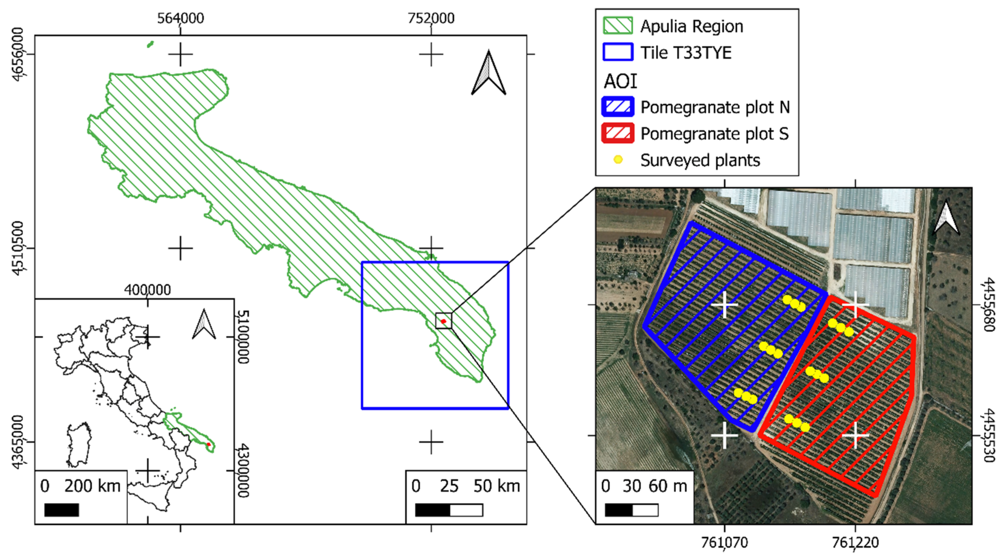
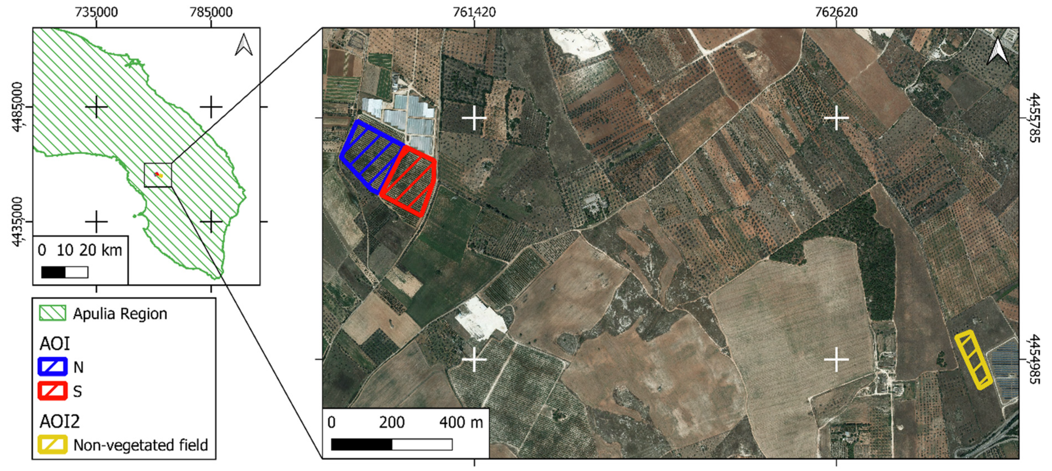
2.1. Study Area and Pilot Plots

The present trial is part of a broader multiyear research project, which involves several aspects of pomegranate cultivation. The area of investigation (AOI) is located in the Apulia region (southeast Italy) and is centered on the organic commercial pomegranate orchard (cv. Acco) of the Durante farm (40°12′36″ N; 18°04′07″ E) in Nardò (Lecce province). Within this area, 2 adjacent pilot plots, both about 2.5 ha in size, were selected and labelled as plot N (north) and plot S (south), respectively, according to their relative position (Figure 1). The soil of both plots has a sandy-loam texture (USDA soil classification); the distance between trees is 1.75 m within rows and 6 m between rows; the tree canopy can be assumed to be a continuous strip about 3 m wide. The tree rows were established on raised beds and mulched by a white plastic foil; the trees were trained to transverse Y trellis system. During the trial, the soil between rows was managed by periodic plowings.

Starting from late June, pilot plots N and S were drip-irrigated with a time frequency of 2–3 days. The irrigations were completed by 10:00 am. Water release was operated through emitters positioned at 50 cm intervals along a single-line pipe laid parallel to the row under the plastic mulch. In accordance with the broader research project, a specific irrigation restriction was applied, in summer 2021, during the period of fruit linear growth, to assess its effect on the water status of pomegranate trees: plot S received about 60% of the standard farm irrigation, about 20 m³/ha every 2–3 days, while plot N was irrigated with the full amount of water on the same days. This period lasted from 28 June to 30 July.

From 18 to 20 July, unusual rainfalls occurred and provided about 62 mm of additional water. In the first half of August 2021, about 32 m³/ha of water was supplied every 2–3 days to both plots in accordance with standard farm management. The dates of drip irrigation and rainfall are provided in

Table 1. Irrigation and rainfall during the trial period.

Date	Irrigation of Plot N (m3 ha−1)	Irrigation of Plot S (m3 ha−1)	Rainfall (mm)
23 June	0.0	0.0	0.0
28 June	21.2	12.6	0.0
1 July	21.2	12.7	0.0
4 July	19.1	11.4	0.0
7 July	19.2	11.5	0.0
9 July	19.2	11.4	0.0
11 July	19.3	11.4	0.0
13 July	19.1	11.5	0.0
15 July	19.2	11.4	0.0
17 July	19.2	11.3	0.0
18 July	0.0	0.0	20.2
19 July	0.0	0.0	38.2
20 July	0.0	0.0	3.5
22 July	16.3	9.6	0.0
24 July	16.1	9.5	0.0
26 July	18.2	10.9	0.0
28 July	19.2	11.4	0.0
30 July	19.3	11.3	0.0
1 August	31.5	32.0	0.0
3 August	32.0	31.8	0.0
5 August	32.4	32.6	0.0
7 August	31.8	31.5	0.0
9 August	30.0	32.0	0.0
11 August	32.5	32.2	0.0
13 August	32.0	31.5	0.0

. All additional cultural practices were uniformly applied to the two plots during the entire growing season, according to the farm’s standard procedures.

2.2. Ground Measurements

Ψ_stem was measured using a pressure chamber (model 3005, Soilmoisture Equip. Corp, Santa Barbara, CA, USA). Measurements were taken for 9 trees per plot (each at least 10 m apart) as single replicates by sampling two small mature shoots located in the lower part of the canopy on two tertiary scaffolds on opposite sides of each tree. Before the measurements, the shoots were enclosed in two-layer bags (plastic inside and aluminum outside) for 2 h to reach equilibrium. The number of replicates was adjusted to take measurements within about 1 h (11:30 a.m. to 12:30 p.m.), aiming to keep environmental conditions as stable as possible to avoid changes that affect the readings of the physiological parameter Ψ_stem. During the period of irrigation restriction, field surveys were carried out on three dates coinciding with the passage of the Sentinel 2 satellite over the study area: 28 July 2021, 7 August 2021 and 12 August 2021. Outside, that period, the same measurements were taken before the start of irrigation, that is, on 23 June.

The difference between the canopy cover of the trees of the two plots was investigated. Digital pictures of the tree shades were taken at solar noon on 23 June 2021, 28 July 2021, 7 August 2021 and 12 August 2021 and processed with the program GIMP (www.gimp.org, accessed on 24 March 2022), transforming the images into black (vegetation) and white (ground) pixels. The percentage of black pixels was indicative of the ground shaded area, which in turn, is known to be related to the tree leaf area. A GNSS receiver (Leica 1200, Leica Geosystem AG, Heerbrugg, Switzerland) was used to position the ground observations. The survey was conducted in the NRTK (Network Real Time Kinematic) VRS mode using the Puglia Region correction service (http://gps.sit.puglia.it/SpiderWeb/frmIndex.aspx, accessed on 24 March 2022). The average accuracy (3D) was 3 cm [42].

A total of 18 points were finally collected (see Figure 1 for the spatial distribution) for the 4 abovementioned dates.

2.3. Satellite Data

A single S2 tile, namely T33TYE, was used. Four S2 cloud-free images were obtained as close as possible to the dates of the field surveys (23 June 2021, 28 July 2021, 7 August 2021 and 12 August 2021). The images were downloaded from the Copernicus Scientific Open Data Hub (https://scihub.copernicus.eu/, accessed on 12 January 2022) as Level 2A products (at-the-ground reflectance calibrated and orthoprojected in WGS84/UTM). The Sentinel 2 acquisition time was set at around 10:30 a.m. local time. The S2 L2A data were provided as 100 km² tiles and contained a scene classification layer (SCL) alerting about shadowy, cloudy or faulty pixels. The S2 technical features are reported in

Table 2. S2 band technical features: central wavelength, bandwidth, ground sample distance (GSD), radiometric resolution and temporal resolution [43].

Spectral Band	Central Wavelength (nm)	Band Width (nm)	GSD (m)
B1 (Aerosol)	443	20	60
B2 (Blue)	490	65	10
B3 (Green)	560	35	10
B4 (Red)	665	30	10
B5 (Red Edge 5)	705	15	20
B6 (Red Edge 6)	740	15	20
B7 (Red Edge 7)	783	20	20
B8 (Near Infrared)	842	115	10
B8A (Near-Infrared Plateau)	885	20	20
B9 (Water Vapor)	945	20	60
B10 (Cirrus)	1380	30	60
B11 (Short-Wave Infrared 1)	1610	90	20
B12 (Short-Wave Infrared 2)	2019	180	20
Radiometric resolution	12 bit
Temporal resolution	5 days

.

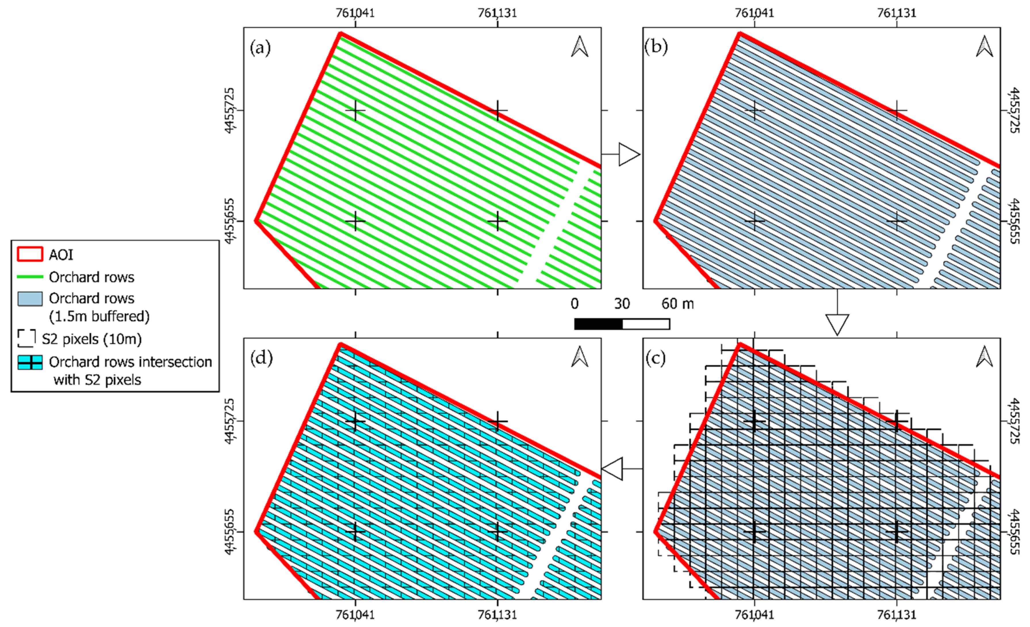
2.4. Data Processing

The Ψ_stem data from plots N and S were compared (i) for a single date and (ii) as aggregated dates to test the significances of both instantaneous differences, which refers to a single date, and differences over the trial period, respectively. A comparison of the group mean values was obtained using a t-test. The significance of differences was tested at p < 0.05. The data were processed by the PAST v. 3.24 software. A point vector file (shapefile format) was then generated from the available GNSS measurements to locate Ψ_stem values in the plots at the right positions, making a direct comparison with S2 data possible.

During S2 data processing, the native bands with 20 m GSD were initially oversampled (bilinear resampling) to 10 m. This pixel size, if considered with respect to the abovementioned canopy and orchard structure, appears to introduce a high degree of noise in the pomegranate interpretation. In fact, the spectral signature of a single S2 pixel has to be considered a “mixed” one, resulting from the joint contribution of both pomegranate canopy and inter-row space (mostly bare soil in AOI); a scheme is given in Figure 2.

Consequently, a first issue to consider recovering the potential “pure” signal for the pomegranate canopy only. The hypothesis is that, with no pure signal recovered, all deductions would be inaccurate and, possibly, misleading. This task is somehow different form the ordinary spectral unmixing (SU) problem [41]. In fact, ordinary SU relies on a priori knowledge of (i) the type of cover class that is expected to participate in the generation of the “recorded” mixed pixel and (ii) the pure spectrum of the cover classes involved. Ordinarily, SU gives an estimate of the percentage of contribution of each class to the recorded signal.

In this study, we needed to recover the pure signal of pomegranate (V) assuming that both the local percentage of area contribution from the two involved classes (pomegranate canopy and bare soil of inter-rows) and the spectrum of the pure local bare soil (S) at the pixel level are known. The spectral un-mixing problem for this study can, therefore, be described by Equation (1):

$${\mathrm{F}}_{\mathrm{i}}\left(\mathrm{x},\mathrm{y}\right)=\mathsf{\alpha }\left(\mathrm{x},\mathrm{y}\right)·{\mathrm{S}}_{\mathrm{i}}+\mathsf{\beta }\left(\mathrm{x},\mathrm{y}\right)·{\mathrm{V}}_{\mathrm{i}}\left(\mathrm{x},\mathrm{y}\right)$$

(1)

where F_i(x,y) is the local reflectance value of the i-th band from S2 data, S_i is the reference reflectance value of the i-th band for the bare soil class, V_i(x,y) is the desired estimate of the local pomegranate reflectance of the i-th band; and α(x,y) and β(x,y) are the numerical parameters representing the local partial contribution of S and V to the mixed signal F. They are assumed to vary locally but remain the same for all the bands.

Since the unknown parameter in the problem is the pure V(x,y) spectrum, Equation (1) can be inverted according to Equation (2):

$${\mathrm{V}}_{\mathrm{i}}\left(\mathrm{x},\mathrm{y}\right)=\frac{{\mathrm{F}}_{\mathrm{i}}\left(\mathrm{x},\mathrm{y}\right)–\mathsf{\alpha }\left(\mathrm{x},\mathrm{y}\right){\mathrm{S}}_{\mathrm{i}}}{\mathsf{\beta }\left(\mathrm{x},\mathrm{y}\right)}$$

(2)

This makes it possible to obtain an estimate of the expected “pure” signal from the pomegranate canopy once the local contributions of V (β) and S (α) are known in terms of the percentage of area within the single S2 pixel.

Based on these premises, a reference spectrum (one for each of the dates considered) of “pure” bare soil was obtained by properly sampling the S2 images available at a location where a bare soil area (AOI2) with a size consistent with S2 geometric resolution was found based on a local inspection. AOI2 was found 1.8 km away from the pilot sites (Figure 3), showing a size of 0.8 ha and being characterized by the same sandy-loam texture (USDA soil classification) of the two pilot plots, which is very common in the area.

Parameters α(x,y) and β(x,y) were locally mapped once the orchard pattern (in terms of the size and direction of the rows) was known and a proper vector graticule was aligned to the S2 tile. The orchard rows were initially represented using a line vector layer interactively edited in QGIS. The rows were interpreted from a high-resolution 2019 aerial orthimage from AGEA (Italian Agency for Payments in Agriculture). The orchard owner confirmed that the orchard pattern did not change between 2019 and 2021. Lines representing the middle of the pomegranate rows were drawn and saved as vector shapefiles. Successively, a buffer of 1.5 m was generated around lines (B) to map the expected area covered by pomegranate canopy (about 3 m wide).

A 10 m squared graticule, perfectly fitting S2 pixels, was then generated (G) and clipped using (B). The resulting layer (C) contains only the parts of the graticule elements potentially filled with pomegranate canopy. For each, the corresponding area was computed using ordinary field calculation tools available in QGIS. The QGIS plugin MMQGIS v. 2021.9.10 was used to operate a spatial join aimed at transferring to (G) the value of the areal contribution of C elements falling within the same (G) feature. A further field computation involving G was finally carried out to derive the local value of β (the fraction of vegetated cover in a pixel) obtained by dividing the previous value by the area of a single S2 pixel (100 m²). Consequently, α was obtained as (1-β). The entire process is graphically shown in Figure 4.

The updated G layer was further completed with the local reflectance values from the S2 bands for all 4 dates considered, making it possible to couple spectral information (F) with the areal one (α and β). Given the previously mentioned reference spectra for bare soil, Equation (2) was applied for each G element and the local estimate of reflectance values of the “pure” pomegranate generated, including the ones at the position of the surveyed plants.

For the interpretation of spectra for predicting agronomic parameters (i.e., ${\mathsf{\Psi }}_{\mathrm{stem}}$), according to the literature, the adoption of appropriate vegetation indices (VIs) appeared to be the most promising one. VIs are in fact able to provide information on crop phenology, growth rate, physiological stresses, etc. [44].

For this study, 2 VIs were selected based on their renowned ability to investigate crop phenology, growth rate and chlorophyll content: (i) the normalized difference vegetation index (NDVI) and (ii) the normalized difference red-edge index (NDRE) [26,45,46,47].

One additional water index, namely the normalized difference water index (NDWI) [47,48], was considered since water-content monitoring is the main issue of this research.

All of the selected indices, given their formulation (see

Table 3. Spectral indices used for this work.${\mathsf{\rho }}_{\mathrm{b}3}$, ${\mathsf{\rho }}_{\mathrm{b}4}$, ${\mathsf{\rho }}_{\mathrm{b}5}$, ${\mathsf{\rho }}_{\mathrm{b}8}$, ${\mathsf{\rho }}_{\mathrm{b}11}$ and ${\mathsf{\rho }}_{\mathrm{b}12}$ are the bottom of atmosphere (BOA) reflectance values for S2 bands 3, 4, 5, 8, 11 and 12, respectively.

Spectral Index Name	Formula
Normalized Difference Vegetation Index	NDVI = $\frac{{(\mathsf{\rho }}_{\mathrm{b}8}-{\mathsf{\rho }}_{\mathrm{b}4})}{\left({\mathsf{\rho }}_{\mathrm{b}8}+{\mathsf{\rho }}_{\mathrm{b}4}\right)}$
Normalized Difference Red-Edge Index	NDRE = $\frac{({\mathsf{\rho }}_{\mathrm{b}8}-{\mathsf{\rho }}_{\mathrm{b}5})}{\left({\mathsf{\rho }}_{\mathrm{b}8}+{\mathsf{\rho }}_{\mathrm{b}5}\right)}$
Normalized Difference Water Index	NDWI = $\frac{({\mathsf{\rho }}_{\mathrm{b}3}-{\mathsf{\rho }}_{\mathrm{b}11})}{\left({\mathsf{\rho }}_{\mathrm{b}3}+{\mathsf{\rho }}_{\mathrm{b}11}\right)}$

), ranged between −1 and +1. In particular, higher NDVI and NDRE values corresponded to highly vegetated/active areas, and high NDWI values indicated high leaf water content or plant water status.

VIs were computed from both native and modified (“pure”) spectra, thus generating two datasets of VIs (namely, VI_M and VI_U) and NDWI (namely, NDWI_M and NDWI_U).

Surveyed plant positions were used to extract the corresponding NDVI, NDRE and NDWI values to characterize the local spectral properties.

To investigate the capability of obtaining spectral information from indices to distinguish ordinarily irrigated plants (plot N) from the ones receiving a reduced water volume (plot S), a t-test and F-test were performed with respect to the mean and variance values of the two groups for both native and pure datasets. A comparison was performed with reference to both the single dates (4 tests) and to the aggregated measures (i.e., 1 test including all observations for the 4 dates).

2.5. Relationships between Ground and Satellite Data through Regression Models

The Ψ_stem values on surveyed plants were directly compared using regression models with both native and pure spectral indices and single bands. Additionally, using a similar approach proposed in [47], the following ratios were computed for both native and pure bands:

$${\tau }_1=\frac{{\mathsf{\Psi }}_{\mathrm{stem}}}{{\mathrm{NDVI}}_{\mathrm{M}}}$$

(3)

$${\tau }_2=\frac{{\mathsf{\Psi }}_{\mathrm{stem}}}{{\mathrm{NDRE}}_{\mathrm{M}}}$$

(4)

$${\tau }_3=\frac{{\mathsf{\Psi }}_{\mathrm{stem}}}{{\mathrm{NDVI}}_{\mathrm{U}}}$$

(5)

$${\tau }_4=\frac{{\mathsf{\Psi }}_{\mathrm{stem}}}{{\mathrm{NDRE}}_{\mathrm{U}}}$$

(6)

The generic τ_i ratio was tested against NDWI and against all of the available S2 bands for both the native and pure datasets. The 1st order polynomial of Equation (7) was used to model all of the relationships:

$$\widehat{{\tau }_{i }}=\widehat{a} ·x+\widehat{b}$$

(7)

where $\widehat{a}$ and $\widehat{b}$ are the “best” estimates of model coefficients, and x is the generic predictor (NDWI or single band).

An estimate of Ψ_stem can be obtained from the ratios by inverting Equation (7) and by replacing ${\tau }_{i }$with $\widehat{{\tau }_{i }}$ (Equation (8))

$${\hat{\mathsf{\Psi }}}_{\mathrm{stem}}=\widehat{{\tau }_{i }}·VI=\left( \widehat{a} x+\widehat{b}\right)·VI$$

(8)

where ${\hat{\mathsf{\Psi }}}_{\mathrm{stem}}$ is the estimated Ψ_stem and VI is the generic vegetation index used to build the ratio.

To test the capability of the regression models of predicting Ψ_stem, the mean absolute error (MAE, Equation (9)) and NMAE (Normalized MAE, Equation (10)) were used as quality measures to compare the estimates with the observed values of Ψ_stem.

$$MAE=\frac{{{\displaystyle \sum }}_{i=1}^N{\left|x_{obs}-x_{est}\right|}_i}{N}$$

(9)

$$NMAE=\frac{MAE}{mean\left(x_{obs}\right)}$$

(10)

where $\left|x_{obs}-x_{est}\right|$ is the absolute difference between the observed water potential (Ψ_stem) and the estimated one (${\hat{\mathsf{\Psi }}}_{\mathrm{stem}}$).

Given the low number of available observations, we decided to use them all to calibrate the predicting models and to approach the validation step using the Leave One Out strategy [49]. In this way, all of the observations, alternatively, were used as members of the validation set to compute both MAE and NMAE.

3. Results

3.1. Testing Ψ_stem and Ground Shaded Area Differences between Plots S and N

The observed stem water potential values ranged from −0.78 MPa in plot N on 12 August to −1.66 MPa in plot S on 23 June. Ψ_stem proved to always be lower in plot S than in plot N. A first analysis aimed to test if any significant difference affects the Ψ_stem values from ground measures taken in plots S and N (

Table 4. The stem water potential differences (ground measures) between plots N and S. Comparisons (t-test) were carried out for both the single-date measures and globally (all dates were jointly considered). Standard deviation, and maximum and minimum values of Ψ_stem measurements are also reported. Significance of tests was set at p < 0.05.

	Plot	t-Test p-Value	Mean	Standard Deviation	Max Ψstem	Min Ψstem
23 June 2021	N	0.120	−1.41	0.09	−1.18	−1.58
	S		−1.47	0.07	−1.30	−1.66
28 July 2021	N	0.450	−1.36	0.11	−1.12	−1.52
	S		−1.40	0.08	−1.24	−1.58
7 August 2021	N	0.050	−1.18	0.17	−0.82	−1.42
	S		−1.35	0.17	−1.06	−1.64
12 August 2021	N	0.008	−1.07	0.12	−0.78	−1.23
	S		−1.22	0.08	−1.01	−1.38
Global	N	0.008	−1.25	0.18	−0.78	−1.58
	S		−1.36	0.15	−1.01	−1.66

). Comparisons at the single-date level proved that, on 23 June and 28 July 2021 (first and second dates), the Ψ_stem differences between plots were not significant. Differences of about 0.06 and 0.04 MPa, respectively, were found, corresponding to percentage difference of about 4 and 3%. On 7 and 12 August 2022 (third and fourth dates); on the contrary, the Ψ_stem difference between plots was found to be significant. Differences of 0.17 and 0.15 MPa, corresponding to percentage differences of about 14% and 12%, respectively, were found. Considering all of the dates together, the Ψ_stem of plots N and S showed a significant difference of 0.11 MPa, corresponding to a percentage difference of about 8%. The portion of ground shaded by pomegranate canopies was different for the 2 plots. As an average of the four dates of measurements, the percentage of shaded soil in plot S exceeded that in plot N by about 17%.

3.2. Vegetation Indices Analyses

With reference to spectral measures from the satellite, the values for plots S and N were compared to test if any significant spectral difference could be found. Again, the tests were carried out at the single-date and global levels.

Table 5. VI_M, VI_U, NDWI_M and NDWI_U statistics of plots N and S over single and aggregated surveys (significance p < 0.05).

		NDVIM		NDVIU
Survey	Plot	t-Test p-Value	Mean	t-Test p-Value	Mean
23 June 2021	N	0.67	0.28	0.95	0.44
	S		0.28		0.44
28 July 2021	N	0.18	0.29	0.18	0.39
	S		0.27		0.35
07 August 2021	N	0.35	0.35	0.11	0.60
	S		0.34		0.53
12 August 2021	N	0.83	0.36	0.44	0.62
	S		0.36		0.59
Global	N	0.62	0.32	0.23	0.52
	S		0.32		0.49
		NDREM		NDREU
	Plot	t-test p-Value	Mean	t-test p-Value	Mean
23 June 2021	N	0.58	0.17	0.64	0.24
	S		0.17		0.25
28 July 2021	N	0.21	0.17	0.21	0.22
	S		0.15		0.18
7 August 2021	N	0.25	0.24	0.12	0.39
	S		0.21		0.31
12 August 2021	N	0.63	0.24	0.33	0.40
	S		0.23		0.34
Global	N	0.29	0.21	0.13	0.32
	S		0.19		0.28
		NDWIM		NDWIU
	Plot	t-test p-Value	Mean	t-test p-Value	Mean
23 June 2021	N	0.00	−0.53	0.00	−0.54
	S		−0.49		−0.47
28 July 2021	N	0.51	−0.50	0.56	−0.42
	S		−0.49		−0.41
7 August 2021	N	0.07	−0.62	0.06	−0.67
	S		−0.59		−0.60
12 August 2021	N	0.06	−0.62	0.05	−0.66
	S		−0.59		−0.59
Global	N	0.06	−0.57	0.03	−0.59
	S		−0.54		−0.53

provides the summary statistics of the t-test aiming to test the differences in the spectral indices considered between plots N and S. During the first survey (23 June), no significant difference was detected by NDVIs and NDREs; conversely, NDWIs detected significant differences. All spectral indices found no differences during the second survey (28 July).

Similar results were obtained for the third and fourth surveys (7 August and 12 August) although NDWI_M and NDWI_U showed p-values very close to the significance limit of 0.05 (7 August: 0.07 and 0.06 for NDWI_M and NDWI_U, respectively; 12 August: 0.06 and 0.05 for NDWI_M and NDWI_U, respectively). In general, NDWIs showed lower values in plot N than in plot S.

Similarly, the t-test conducted for aggregated measures on NDVIs and NDREs showed no significant differences, while the NDWI_M p-value was very close to the significance limit (p = 0.06) and NDWI_U was significant (p = 0.03). Comparing these results with the ones in Table 4 confirms the ability of NDWI to detect differences in leaf water content.

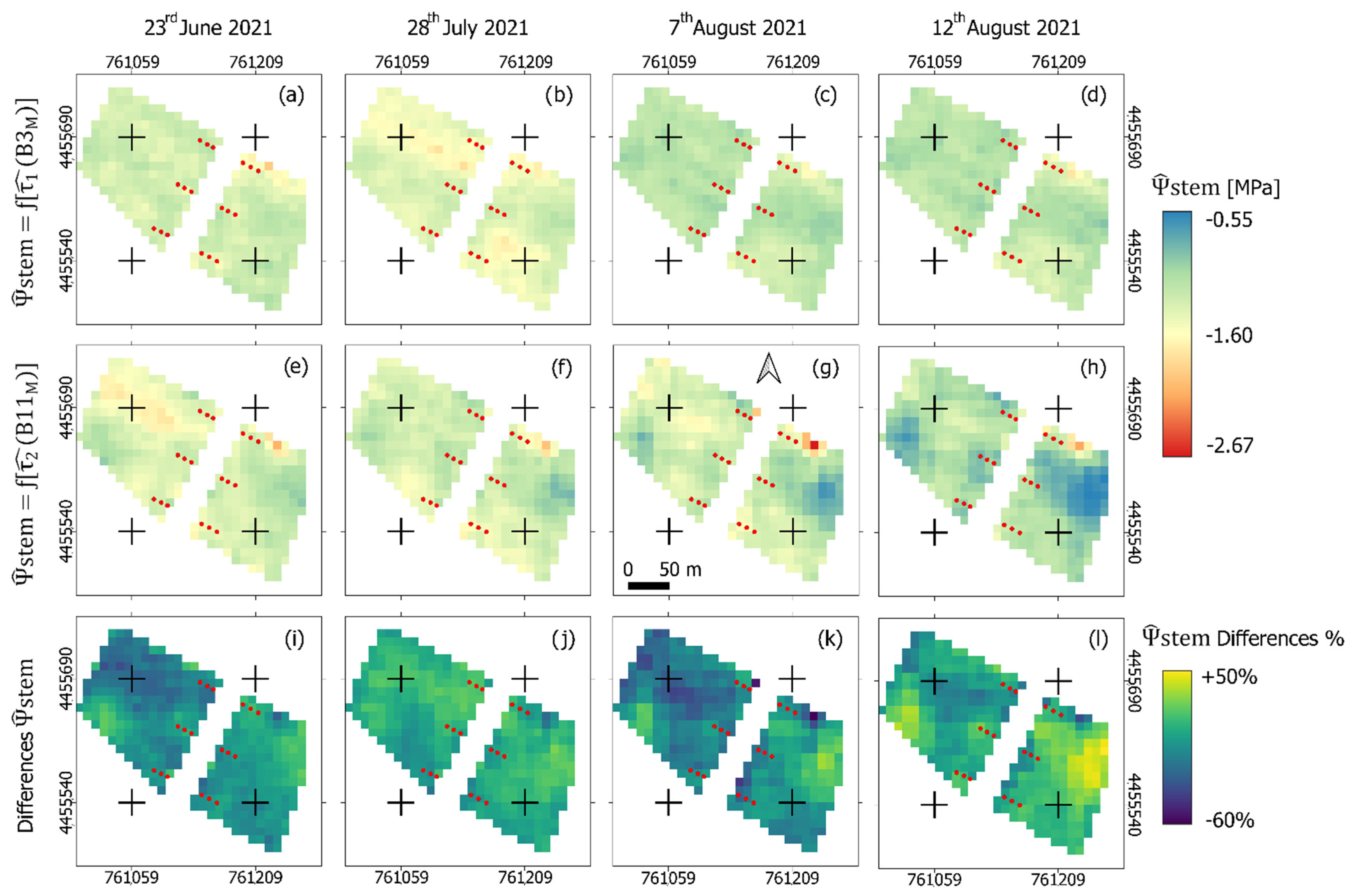
3.3. Relating Ground to Satellite Data through Regression Models

Relating Ψ_stem to spectral bands, VIs and NDWI through regression models led to poor results; in fact, no strong correlation was found for both the “pure” and “mixed” values. However, ${\hat{\mathsf{\Psi }}}_{\mathrm{stem}}$ was reasonably estimated when using $\widehat{{\tau }_{i }}$. The results are reported in

Table 6. Statistics concerning the $\widehat{{\tau }_{1 }}$ and $\widehat{{\tau }_{2 }}$ estimates by Equation (7). SE = standard error, r = Pearson correlation coefficient, R² = coefficient of determination. Predictors are native (“mixed”) bands and spectral indices. B8, B4, B5, NDVI and NDRE were not considered (n/a).

Predictor	τ1						τ2
	a		b		r	R2	a		b		r	R2
	Value	SEa	Value	SEb			Value	SEa	Value	SEb
B2M	−51.30	4.24	−1.19	0.26	−0.84	0.70	−106.55	10.97	−0.75	0.67	−0.77	0.59
B3M	−43.38	2.89	−25	0.27	−0.88	0.78	−91.65	7.68	1.35	0.72	−0.83	0.69
B4M	n/a	n/a	n/a	n/a	n/a	n/a	−84.08	6.07	3.49	0.77	−0.87	0.75
B5M	−24.44	2.77	−0.26	0.45	−0.74	0.55	n/a	n/a	n/a	n/a	n/a	n/a
B6M	−24.43	3.45	1.13	0.76	−0.66	0.44	−69.50	5.62	8.16	1.24	−0.84	0.70
B7M	−24.04	3.48	1.57	0.84	−0.65	0.42	−68.07	5.85	9.34	1.14	−0.82	0.68
B8M	n/a	n/a	n/a	n/a	n/a	n/a	n/a	n/a	n/a	n/a	n/a	n/a
B8AM	−24.65	3.71	2.56	0.98	−0.65	0.43	−70.92	6.52	11.70	1.73	−0.81	0.65
B11M	−28.54	3.66	4.87	1.17	−0.70	0.49	−84.47	4.47	19.86	1.42	−0.92	0.85
B12M	−30.26	3.83	2.98	0.91	−0.70	0.49	−84.33	5.92	13.02	1.41	−0.87	0.76
NDVIM	n/a	n/a	n/a	n/a	n/a	n/a	37.79	3.54	−19.10	1.15	0.80	0.64
NDREM	11.05	1.84	−6.43	0.38	0.6	0.36	n/a	n/a	n/a	n/a	n/a	n/a
NDWIM	−14.97	1.10	−12.58	0.62	−0.86	0.74	−27.03	3.51	−22.13	1.97	−0.69	0.48

and

Table 7. Statistics concerning the $\widehat{{\tau }_{3 }}$ and $\widehat{{\tau }_{4 }}$ estimates by Equation (7). SE = standard error of the parameters, r = Pearson correlation coefficient, R² = coefficient of determination. Predictors are “pure” bands and spectral indices. B8, B4, B5, NDVI and NDRE were not considered (n/a).

Predictor	τ3						τ4
	a		b		r	R2	a		b		r	R2
	Value	SEa	Value	SEb			Value	SEa	Value	SEb
B2U	−25.83	1.78	−1.35	0.11	−0.87	0.77	−58.04	6.27	−1.95	−0.40	−0.76	0.57
B3U	−22.03	1.29	−0.83	0.12	−0.91	0.82	−52.08	4.48	−0.56	0.43	−0.84	0.70
B4U	n/a	n/a	n/a	n/a	n/a	n/a	−47.89	3.66	−0.72	0.37	−0.85	0.72
B5U	−11.65	1.30	−1.04	0.21	−0.74	0.55	n/a	n/a	n/a	n/a	n/a	n/a
B6U	−10.44	1.67	−0.24	0.42	−0.61	0.38	−36.80	3.05	3.80	0.76	−0.84	0.70
B7U	−10.20	1.67	−0.01	0.46	−0.61	0.37	−35.75	3.14	4.65	0.87	−0.84	0.67
B8U	n/a	n/a	n/a	n/a	n/a	n/a	n/a	n/a	n/a	n/a	n/a	n/a
B8AU	−10.94	1.81	0.44	0.54	−0.60	0.36	−37.69	3.55	5.92	1.06	−0.80	0.64
B11U	−13.74	1.56	1.29	0.47	−0.74	0.55	−44.85	2.21	8.11	0.66	−0.93	0.86
B12U	−15.27	1.44	0.54	0.32	−0.80	0.64	−44.68	2.82	4.57	0.61	−0.90	0.81
NDVIU	n/a	n/a	n/a	n/a	n/a	n/a	15.27	1.53	−12.90	0.80	0.78	0.61
NDREU	5.14	0.82	−4.33	0.23	0.67	0.44	n/a	n/a	n/a	n/a	n/a	n/a
NDWIU	−7.45	0.54	−6.94	0.31	−0.86	0.75	−14.38	2.15	−13.20	1.22	−0.64	0.41

. It is worth remembering that $\widehat{{\tau }_{i }}$ (estimate of τ_i) already summarizes the spectral content of both VIs and bands (see Table 3 and Equation (7)). For this reason, B8, B4, B5, NDVI and NDRE were not used as predictors (Equation (7)) of the corresponding $\widehat{{\tau }_{i }}$.

Table 6 shows the following good correlations: τ₁ vs. B2_M (R² = 0.70), τ₁ vs. B3_M (R² = 0.78) and τ₁ vs. NDWI_M (R² = 0.74). Unsatisfying correlations were found between τ₁ and the other bands and spectral indices.

Concerning R², the following good correlations were found: τ₂ vs. B4_M (R² = 0.75), τ₂ vs. B6_M (R² = 0.70), τ₂ vs. B11_M (R² = 0.85) and τ₂ vs. B12_M (R² = 0.76). This suggests that medium infrared bands showed the best ability to predict water potential. Unsatisfying correlations were found between τ₂ and the other bands and spectral indices.

Table 7 reports the parameters and statistics of the model (Equation (7)) for τ_i, with the “pure” bands and indices. The results demonstrate a general improvement in the estimates while working with de-noised spectral measures. The following R² values were, in fact, found for τ₃, with B2_U, B3_U and NDWI_U: 0.77, 0.82 and 0.75, respectively.

Similarly, models for the τ₄ estimate proved to perform slightly better when working with de-noised measures. The following good correlations were, in fact, found in the visible and red-edge regions: τ₄ vs. B3_U (R² = 0.70), τ₄ vs. B4_U (R² = 0.72) and τ₄ vs. B6_U (R² = 0.70). Again, medium infrared bands proved to have the best predictive capacity: τ₄ vs. B11_U (R² = 0.86) and τ₄ vs. B12_U (R² = 0.81).

Whatever the approach (based on native or de-noised spectral measures), it can be noticed that the correlation of τ_i with bands/indices is, generally, negative (r < 0). The only exception comes from NDRE, which once more, demonstrates the synthesis of features of vegetation different from NDVI. Negative correlation values suggest that, generally, plant water status increases when reflectance decreases (or spectral index), thus confirming the absorption capability of water. It is, therefore, reasonable to interpret the higher prediction power of the medium infrared bands as being correlated with their well-known sensitivity to the water content of surfaces.

With reference to the best performing models for τ_i prediction (R² ≥ 0.7), the corresponding Ψ_stem estimates were generated. The associated MAE and NMAE values were therefore computed (see

Table 8. Mean absolute errors (MAE) and normalized MAE values, as computed for the best performing models for the τ_i estimate (n/a = result not compliant with model performance, i.e., R² of the model for τ_i estimate < 0.7).

Predictor	$\widehat{{\mathit{\tau }}_{1 }}$		$\widehat{{\mathit{\tau }}_{2 }}$		$\widehat{{\mathit{\tau }}_{3 }}$		$\widehat{{\mathit{\tau }}_{4 }}$
	MAE (MPa)	NMAE (%)	MAE (MPa)	NMAE (%)	MAE (MPa)	NMAE (%)	MAE (MPa)	NMAE (%)
B2	0.131	−10.0	n/a	n/a	0.172	−13.2	n/a	n/a
B3	0.106	−8.1	n/a	n/a	0.131	−10.1	0.261	−20.0
B4	n/a	n/a	0.139	−10.7	n/a	n/a	0.257	−19.8
B6	n/a	n/a	0.175	−13.5	n/a	n/a	0.256	−19.7
B11	n/a	n/a	0.113	−8.7	n/a	n/a	0.149	−11.5
B12	n/a	n/a	0.142	−10.9	n/a	n/a	0.188	−14.4
NDWI	0.130	−9.9	n/a	n/a	0.192	−14.7	n/a	n/a

) to test their prediction capability.

Table 8 shows that the ${\hat{\mathsf{\Psi }}}_{\mathrm{stem}}$ values obtained using $\widehat{{\tau }_{1 }}\left(B{3}_M\right)$and $\widehat{{\tau }_{2 }}\left(B{11}_M\right)$ as predictors are the most accurate ones. Conversely, $\widehat{{\tau }_{3 }}$ and $\widehat{{\tau }_{4 }}$, although showing better correlations with bands and indices (compare Table 6 and Table 7), led to less accurate results. This means that native data appear to perform better when predicting local water potential conditions than de-noised ones. Although it remains to be confirmed with other more representative tests, this finding suggests that the joint effects of the soil–plant system and its related spectral response are probably more representative of the local water-related dynamics. From an operational point of view, these findings can be translated in maps able to give an estimate of the local expected stem water potential. To make this evident for the case study, a map of ${\hat{\mathsf{\Psi }}}_{\mathrm{stem}}$ was generated for the four sample dates using the following two models: one based on $\widehat{{\tau }_1}\left(B{3}_M\right)$ and the other ones based on $\widehat{{\tau }_2}\left(B{11}_M\right)$. For each date, the maps of differences between the two approaches were also generated (Figure 5i–l). They show no negligible differences in reaching their maximum (about ±50%) during the growing season (up until 12 August). The value of differences cannot entirely be associated with the joint contribution of the estimated uncertainty of each of the maps compared (expected value is around 14% according to the Variance Propagation Law [50]). Consequently, the resulting differences highlight a low degree of robustness of the estimates, making them highly dependent on the predictor adopted.

4. Discussion

Midday stem water potential is well-known as a sensitive indicator of plant water status [23,51]. In previous studies, the Ψ_stem of non-water-stressed pomegranate trees was found to vary from −0.73 to −0.98 MPa [52] or to decrease from −0.6 to −1.5 MPa mid-season, when vapor pressure deficits increased [19]. In the same studies, the Ψ_stem of stressed trees dropped to −1.98 MPa at the end of a water-withholding period [52], to −2.0 MPa when irrigation was managed with a sustained deficit or to −2.4 MPa when irrigation was managed with a regulated deficit [19]. In the present study, Ψ_stem ranged from −0.78 MPa (plot N, 12 August) to −1.66 MPa (plot S, 23 June); these values, compared with the ones reported above, indicate a light level of water deficit for trees of both plots. This consideration is consistent with what was reported in a recent review on the effect of water deficits on pomegranate trees. According to this report, Ψ_stem values between −0.98 and −1.23 MPa indicate no/minimal water deficit, while values between −1.5 and −1.8 MPa indicate a mild/moderate level of water deficit, and values from −1.9 to −2.8 MPa account for a severe/strong water deficit [20]. Regarding the single-date data, the small difference between Ψ_stem of plots N and S found on 23 June and 28 July (i.e., before and at the end of the period in which the amount of irrigation in plot S was restricted) can be explained by the complete absence of irrigation for the first date and by the rainfall that occurred in the second half of July, flattening the tree water status for the second date. On the third (7 August) and fourth (12 August) dates of measurement, i.e., after the end of the differentiation of irrigation between the two plots, the lower Ψ_stem values of plot S indicated a lower water status, which can be explained by the greater leaf surface attributable to these trees based on their canopy shadow.

As far as estimating the capability of these spectral measures is concerned, it was found that spectral signals from the green (B3) and the medium infrared (B11) bands are the best performing ones, making the generation of Ψ_stem estimates with an MAE and an NMAE of about 0.11 MPa and 9%, respectively, possible. These results confirm the association of NDWIs and short-wave infrared (SWIR) bands with tree water status, as found in other studies [53,54]. The approach followed in this test provides sufficiently reliable results despite having a limited amount of data (18 ground measurements for four dates), consistent with the objective of the present study: to develop an easy, fast and cost-effective methodology to map Ψ_stem over the orchard. Other studies tried to estimate Ψ_stem using a multi-seasonal approach, obtaining similar results using commercial high-resolution imagery (Planet and WorldView-2) [38,39], which are not compliant with the objective of the present study.

S2 imagery is provided at 10 (visible and infrared) and 20 m (red-edge and SWIR) resolution depending on the band. S2 geometric resolution could be inadequate when monitoring orchards with 6 m spacing between rows. To overcome this issue, spectral unmixing was performed in order to extract a “pure” signal from the canopy while excluding the bare soil contribution. Good model performances were achieved when native S2 data were used and slightly worse when de-noised measures were used. Although to be confirmed with other more representative tests, this finding suggests that the joint effects of the soil–plant system and its related spectral responses is probably more representative of the local water-related dynamics. If confirmed, this issue will strengthen, once more, the role of S2 L2A data even for describing the behavior of vegetated discontinued surface such as orchards despite the expected noise from the inter-row areas. Both approaches (based on native and “pure” spectral bands) led to negative correlations between τ_i and various bands/indices, suggesting that reflectance decreases (or spectral indices) when plant water status increases, thus confirming the absorption capability of water. Only NDRE led to positive correlations; therefore, this study confirms that NDRE expresses different vegetation features from NDVI or NDWI.

Regarding the degree of confidence of the Ψ_stem estimates, it was proven to be unsatisfactory for operational purposes, since it is strictly dependent on the predictors selected: τ_i (i.e., spectral index) and spectral bands used to model τ_i (namely, B3 and B11). Nevertheless, some interesting indications come from our tests. The first one concerns the relationship between the spectral index involved in the τ_i computation and the band used as a predictor. In fact, the results suggest that an NDRE-based τ can be better estimated from the mid-infrared bands; conversely, an NDVI-based τ can be better estimated form visible bands (specifically, the green one).

Conclusions: (i) Ψ_stem can be satisfactorily estimated by the ${\hat{\mathsf{\Psi }}}_{\mathrm{stem}}$equation, even with a limited amount of ground data; (ii) native data, despite noise, appear to perform better when predicting local Ψ_stem values than de-noised ones; (iii) predictions based on band 3 (green @ 560) and band 11 (SWIR @ 1610 nm) are the most accurate ones; and (iv) Ψ_stem estimates from different regression methods showed slightly differences in both value and spatial distribution. This alerts us that our deductions are probably not conclusive and, certainly, preliminary. Nevertheless, the approach appears to be promising, and further developments are desirable.

References

1. Spagnoli, F. Ane Today—The Golden Pome: The Pomegranate from Its Deepest Roots to Modern Culture; American Society of Overseas Research (ASOR): Alexandria, VA, USA, 2019. [Google Scholar]
2. Coltivazioni: Coltivazioni Legnose Fruttifere. Available online: http://dati.istat.it/Index.aspx?QueryId=33705 (accessed on 2 May 2022).
3. Herrera, E.; Jiménez, R.; Aruoma, O.I.; Hercberg, S.; Sanchez-Garcia, I.; Fraga, C. Aspects of antioxidant foods and supplements in health and disease. Nutr. Rev. 2009, 67, S140–S144. [Google Scholar] [CrossRef] [PubMed]
4. Cantele, C.; Rojo-Poveda, O.; Bertolino, M.; Ghirardello, D.; Cardenia, V.; Barbosa-Pereira, L.; Zeppa, G. In Vitro Bioaccessibility and Functional Properties of Phenolic Compounds from Enriched Beverages Based on Cocoa Bean Shell. Foods 2020, 9, 715. [Google Scholar] [CrossRef] [PubMed]
5. Cantele, C.; Bertolino, M.; Bakro, F.; Giordano, M.; Jędryczka, M.; Cardenia, V. Antioxidant Effects of Hemp (Cannabis sativa L.) Inflorescence Extract in Stripped Linseed Oil. Antioxidants 2020, 9, 1131. [Google Scholar] [CrossRef] [PubMed]
6. Cantele, C.; Tedesco, M.; Ghirardello, D.; Zeppa, G.; Bertolino, M. Coffee Silverskin as a Functional Ingredient in Vegan Biscuits: Physicochemical and Sensory Properties and In Vitro Bioaccessibility of Bioactive Compounds. Foods 2022, 11, 717. [Google Scholar] [CrossRef] [PubMed]
7. Fraga, C.G.; Croft, K.D.; Kennedy, D.O.; Tomás-Barberán, F.A. The effects of polyphenols and other bioactives on human health. Food Funct. 2019, 10, 514–528. [Google Scholar] [CrossRef] [PubMed]
8. Vauzour, D.; Rodriguez-Mateos, A.; Corona, G.; Oruna-Concha, M.J.; Spencer, J.P.E. Polyphenols and Human Health: Prevention of Disease and Mechanisms of Action. Nutrients 2010, 2, 1106–1131. [Google Scholar] [CrossRef]
9. Malik, A.; Mukhtar, H. Prostate Cancer Prevention Through Pomegranate Fruit. Cell Cycle 2006, 5, 371–373. [Google Scholar] [CrossRef]
10. Lansky, E.P.; Newman, R.A. Punica granatum (pomegranate) and its potential for prevention and treatment of inflammation and cancer. J. Ethnopharmacol. 2007, 109, 177–206. [Google Scholar] [CrossRef]
11. Moccia, S. Pomegranate: A Source of Active Compounds with a Health-Promoting Role. In Punica Granatum: Cultivation, Properties and Health Benefits; Nova Science Publishers, Inc.: Hauppauge, NY, USA, 2021; pp. 21–40. ISBN 978-1-5361-9821-8. [Google Scholar]
12. Bajaj, K.K.; Kale, M.B.; Umare, M.D.; Wankhede, N.L.; Taksande, B.G.; Trivedi, R.V.; Umekar, M.J.; Upaganlawar, A.B. Potential Benefits and Effects of Pomegranate in Metabolic Disorders. In Punica Granatum: Cultivation, Properties and Health Benefits; Nova Science Publishers, Inc.: Hauppauge, NY, USA, 2021; pp. 193–222. ISBN 978-1-5361-9821-8. [Google Scholar]
13. Hmid, I.; Elothmani, D.; Hanine, H.; Oukabli, A.; Mehinagic, E. Comparative study of phenolic compounds and their antioxidant attributes of eighteen pomegranate (Punica granatum L.) cultivars grown in Morocco. Arab. J. Chem. 2017, 10, S2675–S2684. [Google Scholar] [CrossRef]
14. Gundogdu, M.; Yilmaz, H. Organic acid, phenolic profile and antioxidant capacities of pomegranate (Punica granatum L.) cultivars and selected genotypes. Sci. Hortic. 2012, 143, 38–42. [Google Scholar] [CrossRef]
15. Rolle, L.; Giacosa, S.; Gerbi, V.; Bertolino, M.; Novello, V. Varietal Comparison of The Chemical, Physical, and Mechanical Properties of Five Colored Table Grapes. Int. J. Food Prop. 2013, 16, 598–612. [Google Scholar] [CrossRef]
16. Lyu, Y.; Porat, R.; Yermiyahu, U.; Heler, Y.; Holland, D.; Dag, A. Effects of nitrogen fertilization on pomegranate fruit, aril and juice quality. J. Sci. Food Agric. 2020, 100, 1678–1686. [Google Scholar] [CrossRef] [PubMed]
17. Selahvarzi, Y.; Zamani, Z.; Fatahi, R.; Talaei, A.-R. Effect of deficit irrigation on flowering and fruit properties of pomegranate (Punica granatum cv. Shahvar). Agric. Water Manag. 2017, 192, 189–197. [Google Scholar] [CrossRef]
18. Parvizi, H.; Sepaskhah, A.R.; Ahmadi, S.H. Physiological and growth responses of pomegranate tree (Punica granatum L. cv. Rabab) under partial root zone drying and deficit irrigation regimes. Agric. Water Manag. 2016, 163, 146–158. [Google Scholar] [CrossRef]
19. Intrigliolo, D.; Nicolás, E.; Bonet, L.; Ferrer, P.; Alarcon, J.J.; Bartual, J. Water relations of field grown Pomegranate trees (Punica granatum) under different drip irrigation regimes. Agric. Water Manag. 2011, 98, 691–696. [Google Scholar] [CrossRef]
20. Volschenk, T. Effect of water deficits on pomegranate tree performance and fruit quality—A review. Agric. Water Manag. 2021, 246, 106499. [Google Scholar] [CrossRef]
21. Conesa, M.R.; Falagán, N.; de la Rosa, J.M.; Aguayo, E.; Domingo, R.; Pastor, A.P. Post-veraison deficit irrigation regimes enhance berry coloration and health-promoting bioactive compounds in ‘Crimson Seedless’ table grapes. Agric. Water Manag. 2016, 163, 9–18. [Google Scholar] [CrossRef]
22. Galindo, A.; Calín-Sánchez, A.; Griñán, I.; Rodríguez, P.; Cruz, Z.; Girón, I.; Corell, M.; Martínez-Font, R.; Moriana, A.; Carbonell-Barrachina, A.; et al. Water stress at the end of the pomegranate fruit ripening stage produces earlier harvest and improves fruit quality. Sci. Hortic. 2017, 226, 68–74. [Google Scholar] [CrossRef]
23. Lipan, L.; Collado-González, J.; Wojdyło, A.; Domínguez-Perles, R.; Gil-Izquierdo, A.; Corell, M.; Moriana, A.; Cano-Lamadrid, M.; Carbonell-Barrachina, A. How does water stress affect the low molecular weight phenolics of hydroSOStainable almonds? Food Chem. 2021, 339, 127756. [Google Scholar] [CrossRef]
24. Segarra, J.; Buchaillot, M.L.; Araus, J.L.; Kefauver, S.C. Remote Sensing for Precision Agriculture: Sentinel-2 Improved Features and Applications. Agronomy 2020, 10, 641. [Google Scholar] [CrossRef]
25. Hill, M.J. Vegetation index suites as indicators of vegetation state in grassland and savanna: An analysis with simulated SENTINEL 2 data for a North American transect. Remote Sens. Environ. 2013, 137, 94–111. [Google Scholar] [CrossRef]
26. Misra, G.; Cawkwell, F.; Wingler, A. Status of Phenological Research Using Sentinel-2 Data: A Review. Remote Sens. 2020, 12, 2760. [Google Scholar] [CrossRef]
27. De Petris, S.; Sarvia, F.; Borgogno-Mondino, E. A New Index for Assessing Tree Vigour Decline Based on Sentinel-2 Multitemporal Data. Application to Tree Failure Risk Management. Remote Sens. Lett. 2021, 12, 58–67. [Google Scholar]
28. Sarvia, F.; De Petris, S.; Borgogno-Mondino, E. Exploring Climate Change Effects on Vegetation Phenology by MOD13Q1 Data: The Piemonte Region Case Study in the Period 2001–2019. Agronomy 2021, 11, 555. [Google Scholar] [CrossRef]
29. Orusa, T.; Mondino, E.B. Exploring Short-Term Climate Change Effects on Rangelands and Broad-Leaved Forests by Free Satellite Data in Aosta Valley (Northwest Italy). Climate 2021, 9, 47. [Google Scholar] [CrossRef]
30. Orusa, T.; Orusa, R.; Viani, A.; Carella, E.; Mondino, E.B. Geomatics and EO Data to Support Wildlife Diseases Assessment at Landscape Level: A Pilot Experience to Map Infectious Keratoconjunctivitis in Chamois and Phenological Trends in Aosta Valley (NW Italy). Remote Sens. 2020, 12, 3542. [Google Scholar] [CrossRef]
31. Clevers, J.G.P.W.; Gitelson, A.A. Remote estimation of crop and grass chlorophyll and nitrogen content using red-edge bands on Sentinel-2 and -3. Int. J. Appl. Earth Observ. Geoinf. 2013, 23, 344–351. [Google Scholar] [CrossRef]
32. Jopia, A.; Zambrano, F.; Pérez-Martínez, W.; Vidal-Páez, P.; Molina, J.; Mardones, F.D.L.H. Time-Series of Vegetation Indices (VNIR/SWIR) Derived from Sentinel-2 (A/B) to Assess Turgor Pressure in Kiwifruit. ISPRS Int. J. Geo-Inf. 2020, 9, 641. [Google Scholar] [CrossRef]
33. Borgogno-Mondino, E.; Sarvia, F.; Gomarasca, M.A. Supporting Insurance Strategies in Agriculture by Remote Sensing: A Possible Approach at Regional Level. In Proceedings of the International Conference on Computational Science and Its Applications, Saint Petersburg, Russia, 1–4 July 2019; Springer: Berlin/Heidelberg, Germany, 2019; pp. 186–199. [Google Scholar]
34. Shrestha, R.; Di, L.; Yu, E.G.; Kang, L.; Shao, Y.-Z.; Bai, Y.-Q. Regression model to estimate flood impact on corn yield using MODIS NDVI and USDA cropland data layer. J. Integr. Agric. 2017, 16, 398–407. [Google Scholar] [CrossRef]
35. Sarvia, F.; Xausa, E.; De Petris, S.D.; Cantamessa, G.; Borgogno-Mondino, E. A Possible Role of Copernicus Sentinel-2 Data to Support Common Agricultural Policy Controls in Agriculture. Agronomy 2021, 11, 110. [Google Scholar] [CrossRef]
36. Kanjir, U.; Djurić, N.; Veljanovski, T. Sentinel-2 Based Temporal Detection of Agricultural Land Use Anomalies in Support of Common Agricultural Policy Monitoring. ISPRS Int. J. Geo-Inf. 2018, 7, 405. [Google Scholar] [CrossRef] [Green Version]
37. Jamshidi, S.; Zand-Parsa, S.; Niyogi, D. Assessing Crop Water Stress Index of Citrus Using In-Situ Measurements, Landsat, and Sentinel-2 Data. Int. J. Remote Sens. 2021, 42, 1893–1916. [Google Scholar] [CrossRef]
38. Van Beek, J.; Tits, L.; Somers, B.; Coppin, P. Stem Water Potential Monitoring in Pear Orchards through WorldView-2 Multispectral Imagery. Remote Sens. 2013, 5, 6647–6666. [Google Scholar] [CrossRef]
39. Helman, D.; Bahat, I.; Netzer, Y.; Ben-Gal, A.; Alchanatis, V.; Peeters, A.; Cohen, Y. Using Time Series of High-Resolution Planet Satellite Images to Monitor Grapevine Stem Water Potential in Commercial Vineyards. Remote Sens. 2018, 10, 1615. [Google Scholar] [CrossRef]
40. D’Urso, G.; Maltese, A.; Palladino, M.E.O. Based Estimation of Transpiration and Crop Water Requirements for Vineyards: A Case Study in Southern Italy. In Remote Sensing for Agriculture, Ecosystems, and Hydrology XVI; SPIE: Bellingham, WA, USA, 2014; Volume 9239, pp. 257–265. [Google Scholar]
41. Quintano, C.; Fernández-Manso, A.; Shimabukuro, Y.E.; Pereira, G. Spectral unmixing. Int. J. Remote Sens. 2012, 33, 5307–5340. [Google Scholar] [CrossRef]
42. Dardanelli, G.; Maltese, A.; Pipitone, C.; Pisciotta, A.; Brutto, M.L. NRTK, PPP or Static, That Is the Question. Testing Different Positioning Solutions for GNSS Survey. Remote Sens. 2021, 13, 1406. [Google Scholar] [CrossRef]
43. Sentinel-2—Missions Sentinel Online. Available online: https://sentinel.esa.int/web/sentinel/missions/sentinel-2 (accessed on 3 August 2022).
44. Xue, J.; Su, B. Significant remote sensing vegetation indices: A review of developments and applications. J. Sens. 2017, 2017, e1353691. [Google Scholar] [CrossRef]
45. Thompson, C.N.; Guo, W.; Sharma, B.; Ritchie, G.L. Using Normalized Difference Red Edge Index to Assess Maturity in Cotton. Crop Sci. 2019, 59, 2167–2177. [Google Scholar] [CrossRef]
46. Fitzgerald, G.; Rodriguez, D.; O’Leary, G. Measuring and predicting canopy nitrogen nutrition in wheat using a spectral index—The canopy chlorophyll content index (CCCI). Field Crop. Res. 2010, 116, 318–324. [Google Scholar] [CrossRef]
47. Borgogno-Mondino, E.; Novello, V.; Lessio, A.; de Palma, L. Describing the spatio-temporal variability of vines and soil by satellite-based spectral indices: A case study in Apulia (South Italy). Int. J. Appl. Earth Obs. Geoinf. ITC J. 2018, 68, 42–50. [Google Scholar] [CrossRef]
48. Gu, Y.; Brown, J.F.; Verdin, J.P.; Wardlow, B. A five-year analysis of MODIS NDVI and NDWI for grassland drought assessment over the central Great Plains of the United States. Geophys. Res. Lett. 2007, 34, L06407. [Google Scholar] [CrossRef] [Green Version]
49. Brovelli, M.A.; Crespi, M.; Fratarcangeli, F.; Giannone, F.; Realini, E. Accuracy assessment of high resolution satellite imagery orientation by leave-one-out method. ISPRS J. Photogramm. Remote Sens. 2008, 63, 427–440. [Google Scholar] [CrossRef]
50. De Petris, S.; Sarvia, F.; Borgogno-Mondino, E. About Tree Height Measurement: Theoretical and Practical Issues for Uncertainty Quantification and Mapping. Forests 2022, 13, 969. [Google Scholar] [CrossRef]
51. McCutchan, H.; Shackel, K.A. Stem-water Potential as a Sensitive Indicator of Water Stress in Prune Trees (Prunus domestica L. cv. French). J. Am. Soc. Hortic. Sci. 1992, 117, 607–611. [Google Scholar] [CrossRef]
52. Galindo, A.; Rodríguez, P.; Mellisho, C.; Torrecillas, E.; Moriana, A.; Cruz, Z.; Conejero, W.; Moreno, F.; Torrecillas, A. Assessment of discretely measured indicators and maximum daily trunk shrinkage for detecting water stress in pomegranate trees. Agric. For. Meteorol. 2013, 180, 58–65. [Google Scholar] [CrossRef]
53. Gao, B.-C. NDWI—A normalized difference water index for remote sensing of vegetation liquid water from space. Remote Sens. Environ. 1996, 58, 257–266. [Google Scholar] [CrossRef]
54. Ceccato, P.; Flasse, S.; Grégoire, J.-M. Designing a spectral index to estimate vegetation water content from remote sensing data: Part 2. Validation and applications. Remote Sens. Environ. 2002, 82, 198–207. [Google Scholar] [CrossRef]
Figure 1. Apulia region (green lined), located in Southern Italy. Pomegranate plots N and S are represented with blue and red lined polygons, respectively. Yellow dots represent the spatial distribution of surveyed pomegranate plants. The S2 T33TYE tile is represented as a blue square in the left frame (the reference system is WGS 84/UTM 33N, EPSG: 32,633).
Horticulturae 08 00759 g001
Figure 2. (a) Sentinel 2 GSD (red lines) compared with an orchard pattern (within rows + between rows). Graphs (bd) show the effects of the joint spectral contribution of the two classes possibly included in a single S2 pixel: (b) spectral signature of “pure” active vegetation; (c) spectral signature of “pure” bare soil (clay); (d) resulting mixed spectral signature. Spectral signatures (bd) are simply demonstrative (from a ground spectro-radiometer) and used to show the expected spectral effect within a mixed pixel.
Horticulturae 08 00759 g002
Figure 3. Spatial disposition of AOI and AOI2. Pomegranate plots N and S are represented with blue- and red-lined polygons, respectively. The yellow-lined polygon refers to the non-vegetated field. (The reference system is WGS 84/UTM 33N, EPSG: 32,633).
Horticulturae 08 00759 g003
Figure 4. Sequence of GIS operations needed to map the percentage of pomegranate canopy (β) within S2 pixels: (a) orchard row editing (from AGEA orthoimage); (b) buffering (1.5 m width); (c) graticule generation; (d) intersection between graticule and buffers (the reference system is WGS 84/UTM 33N, EPSG: 32633).
Horticulturae 08 00759 g004
Figure 5. Maps of Ψ ^ stem for plots N and S based on τ 1   ^ ( B 3 M ) (ad) and τ 2   ^ ( B 11 M ) (eh). Maps of percentage differences are also reported (il). Maps are given for the sampled dates: 23 June (a,e,i), 28 July (b,f,j), 7 August (c,g,k) and 12 August (d,h,l). Red dots represent the spatial distribution of surveyed pomegranate plants. The reference system is WGS 84 / UTM 33N, EPSG: 32633.
Horticulturae 08 00759 g005