Article

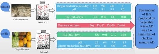
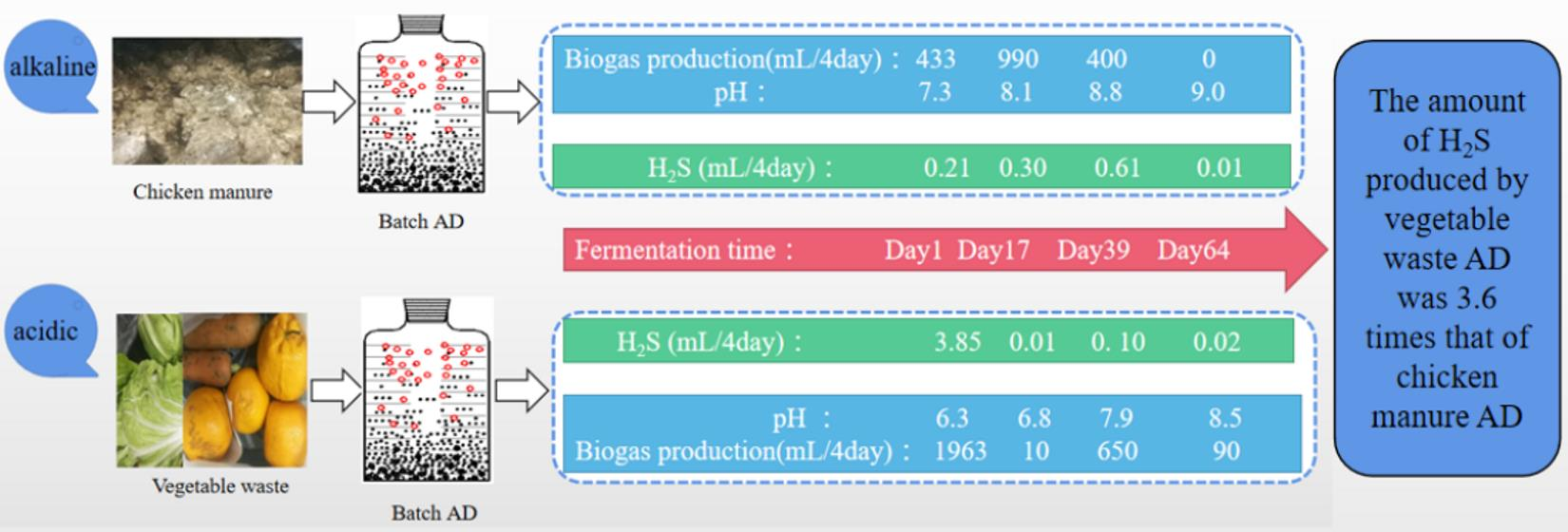
H2S Emission and Microbial Community of Chicken Manure and Vegetable Waste in Anaerobic Digestion: A Comparative Study

1
Key Laboratory of Plant Resource Conservation and Germplasm Innovation in Mountainous Region (Ministry of Education), Institute of New Rural Development, Guizhou University, Guiyang 550025, China
2
Environmental Simulation and Pollution Control State Key Joint Laboratory, School of Environment, Tsinghua University, Beijing 100084, China
3
State Environmental Protection Key Laboratory of Microorganism Application and Risk Control (SMARC), Graduate School at Shenzhen, Tsinghua University, Shenzhen 518055, China
*
Authors to whom correspondence should be addressed.
Fermentation 2023, 9(2), 169; https://doi.org/10.3390/fermentation9020169
Submission received: 4 January 2023 / Revised: 30 January 2023 / Accepted: 2 February 2023 / Published: 13 February 2023
(This article belongs to the Section Industrial Fermentation)

Abstract

:
In order to solve the problem of H2S corrosion in biogas utilization, it is necessary to understand the characteristics and mechanisms of H2S production in chicken manure anaerobic digestion (CMAD) and vegetable waste anaerobic digestion (VWAD). In this study, lab-scale batch tests of CMAD and VWAD were conducted for 67 days at 35 °C. The results showed that sulfide was found to be the major form of sulfur in CMAD (accounting for 90%) and VWAD (70%). The average concentration of H2S was 198 ± 79 ppm in CMAD and 738 ± 210 ppm in VWAD. Moreover, 81% of total H2S was produced at 20 days of methane production in CMAD, but 80% of total H2S was produced in the first day in VWAD because of the rapid production of biogas and fermentation acidification. The sulfide ion equilibrium model could universally and feasibly predict the H2S production in CMAD and VWAD. The abundance of Firmicutes, Bacteroidetes, Proteobacteria and Euryarchaeota accounted for about 95% of the total microbes in both CMAD and VWAD; the influence of the fermentation stage on the microbial community was greater than that of the difference between CM and VW; the abundance of SRB was 0.01~0.07%, while that concerning organosulfur compounds fermentation was 22.8~30.5%. This study indicated that the H2S concentration of CMAD biogas was more than five times that of VWAD because CM is alkalescent but VW is acidic.

Graphical Abstract

1. Introduction

Copious amounts of chicken manure (CM) and vegetable waste (VW) are produced in China, reaching 100–210 million tons and 269 million tons, respectively, in 2015 [1,2]. Improper treatment could result in a foul odor, exposure to toxins and pathogens, etc. Anaerobic digestion (AD) technology has been described as sustainable and is widely applied in the recycling of biogas and fertilizer from CM and VW. The corrosive character of the H2S in biogas is detrimental with respect to using such biogas in engines or boilers. It could be sensible to also mention its influence on systems which are used for upgrading the biogas to biomethane. Moreover, one of the future ways of using biogas could be its reforming and use for subsequent synthesis. For such novel applications, H2S is very problematic due to its detrimental influence to catalysts [3,4,5]. These issues could potentially be overcome by the in situ extraction of problematic substances during AD. Therefore, obtaining further knowledge on the exact processes responsible for the production of these odorants is critical.
Numerous studies of the characteristics of odors produced during the AD of municipal sludge were conducted in the past two decades, thereby identifying H2S as an important contributor of odors and corrosion. Municipal sludge AD typically results in the production of 500–4000 ppm H2S, a byproduct of the hydrolysis of organic sulfurs and reduction of inorganic sulfates [6,7,8]. Numerous studies showed that there were two biochemical ways to form sulfide (including S2−, HS, and H2S) in anaerobic microbial process: one is the reduction of sulfur to an oxidation state such as sulfate by sulfate reduction bacteria (SRB), which can compete with methanogens for substrates such as H2 and acetate during AD; the other is the decomposition of organic sulfur such as protein, methionine, and methyl mercaptan by bacteria and archaea [9,10,11,12].
However, studies on the H2S characteristics of the AD process targeting VW and CM are limited. The differences in metabolism in the anaerobic digestion of CMAD and VWAD, with respect to H2S generation, are not clearly understood. To answer the issues above, in the present study, the abiotic factors and microbial community were detected to compare the characteristics and metabolism of H2S emission in CMAD with those in VWAD.

2. Materials and Methods

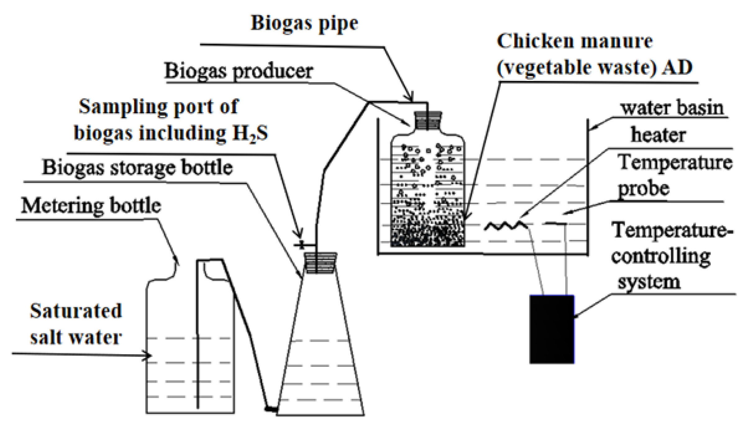
2.1. Experiment Design and Sample Preparation

The present study fermented two kinds of raw materials for batch processing (35 °C), namely, chicken manure (CM) and vegetable waste (VW). Three replicates (three batch biogas reactors) were designed for each raw material. Figure 1 shows the schematics of the reactor. The metering bottles (Shuniu Glass Co., Ltd., Chengdu, China), biogas producer(Shuniu Glass Co., Ltd., Chengdu, China), and storage(Shuniu Glass Co., Ltd., Chengdu, China) all have an equal working volume of 1 L. The volume of fermentation liquor was 0.8 L, its concentration was 5.9%, and the inoculum to raw material total solids (TS) ratio was 2:1. CM was sourced from a chicken farm in Cixi City, Zhejiang Province, China; VW was sourced from a farmers’ market on a university campus in Beijing, China. The inoculum was naturalized using raw materials (CM and VW) over a period of 40 days. The profiles of the raw material and inoculum are reported in Table 1. H2S concentrations and biogas yield were measured each day during peak biogas production and every four days during non-peak production. On days 0, 6, 17, 39, and 67, sludge specimens from the biogas fermenter were even moved into sterilization tubes(Anhui Vincennes Medical Device Co., Ltd., Hefei, China). Samples were stored at −20 °C until extraction of DNA, following which the abiotic factors were determined.

2.2. Determination of Abiotic Factors

The H2S concentrations in biogas were measured using gas chromatography with a Fission-Product Detector (FPD) (GC-14B, Shimadzu Co., Ltd., Kyoto, Japan); the FPD, inject port, and chromatographic column were all set to 240 °C, 100 °C, and 60 °C, respectively; and the carrier gas was nitrogen. CH4 and CO2 were measured with gas chromatography using a Thermal Conductivity Detector (TCD) (GC-14C, Shimadzu Co., Ltd., Kyoto, Japan); inject port, chromatographic column (5 A molecular sieve), and TCD were all adjusted at 60 °C, 60 °C, and 100 °C, respectively; and argon was used as the carrier gas. Sulfate was tested with ion chromatography (type: INTEGRION-HPIC; detector: conductance; separation column: IonPac AS11/HC; guard column: IonPac AG11/HC; leachate: 30 mmol/L KOH; flow velocity: 1 mL/min; current of suppressor: 75 mA; sample size: 25 μL). Using methylene blue spectrophotometry, total sulfides (included S2−, HS, and H2S in fermentation sediment and liquor) and supernatant sulfides were tested. Supernatant sulfide is the sulfide in the upper layer of fermentation broth remaining in centrifugal tube after 5 min. An elemental analyzer was used to test the total sulfur (S-total) by following the manufacturer’s instructions (Flashsmart, Thermo Fisher SCIENTIFIC, Waltham, MA, USA). A Multimeter HACH instrument (HQ40d, HACH)(HACH Water Analysis Instrument (Shanghai) Co., Ltd., Shanghai, China) was used to measure the amount of dissolved oxygen (DO), pH, and oxidoreduction potential (ORP).

2.3. Calculation Formula

2.3.1. H2S Production Prediction Calculation Formula

The prediction of H2S production is based on the sulfide equilibrium model (Supplementary File S1), and the key formulas include:
C H 2 S = 34 S T / ( 32 ( 1 + K S 1 10 p H + K S 1 K S 2 10 2 p H ) )
In Equation (1) CH2S represents the H2S concentration in fermentation liquid (mg/m3), Ks2 = 1.3 × 10⁻⁷ and Ks1 = 7.1 × 10⁻¹⁵ are the secondary and primary H2S ionization constants respectively, and ST represents dissolved sulfide (mg/m3).
C = E C H 2 S
P = C P B i o g a s
In Equations (2) and (3), C is the H2S concentration in biogas (mg/m3), E represents Henry’s constant (0.686 kPa at 35 °C), P (uL/day) represents the daily production of H2S, and PBiogas (mL/day) stands for the daily production of biogas.

2.3.2. Formulas for Biogas and H2S Production Potential

Biogas yield potential was counted based on following formula, which was obtained based on the experience of many batch fermentation studies by others and ourselves [13]:
A = ( B C D ) / E
where A: Biogas yield potential of CM/VW; B: biogas cumulant of CM/VW; C: biogas cumulant of inoculum; D: biogas cumulant of samples of sludge removed; E: total solid of CM/VW.
The potentials of H2S yields of CM/VW are counted based on the following formula:
A = ( i = 0 n a i × b i i = 0 n c i × d i ) / E
where A: H2S production potential of CM/VW; ai: biogas production of CM/VW at day i; bi: H2S concentration of CM/VW at day i; ci: inoculum biogas yield at day i; di: inoculum H2S concentration at day i; E: CM/VW total solids. (Note: The samples of the H2S concentration test were collected from the gas bomb.)

2.4. Characterization of the Microbial Community

Before DNA extraction and high-throughput sequencing, the specimens from reactor replicates were intermingled. Genomic DNA was extracted from samples using cetyltrimethylammonium bromide. The primers (341F (5′-CCTAYGGGRBGCASC AG-3′)/806R (5′-GGACTACNNGGGT ATCTA AT-3′)) were used to amplify the V3–V4 regions of the archaea and bacteria 16S genes [14]. Different samples were identified in labels using barcode sequences. Polymerase chain reaction (PCR) of DNA was performed by sequencing company (Novo gene Biotechnology Co., Ltd. Beijing, China). The PCR products were mixed to the equidensity ratio. The sequencing libraries were generated guided by the manufacturer product description, followeing which the identity codes of each sequence were added. To generate superior-quality data, an Illumina Sequencer called Hiseq PE2500 was utilized, which was subsequently processed using the Qiime2 software program [15]. Cutadapt was used to trim adapter sequences and barcodes [16], which were then truncated at 210 bp and 220 bp, respectively, for reverse and forward reads, merged with 20 bp overlap in DADA2 to form ASV table [17]. At 97 percent similarity to the Naïve Bayes approach, the Greengene database was used for taxonomy classification [18]. For functional predictions, the FAPROTAX database was utilized [19], with vsearch [20] clustering ASVs at 97 percent against the Greengene database used to create taxonomy.

3. Results and Discussion

3.1. Characteristics of CM, VW, and Inoculum

Table 1 shows that sulfide and sulfate were the main forms of sulfur in CM, where S-sulfide accounted for 34.2% of S-total and S-sulfate accounted for 25.6%, while S-protein accounted for 5.2%; CM was weakly alkaline (pH 7.37). Sulfate and protein were the main chemical forms of sulfur in VW, where S-sulfate accounted for 48.5% of S-total and S-protein accounted for 36.1%, while sulfide levels were observed to be very low and were thus ignored due to the extremely high ORP (152 mV) and DO (7.37 mg/L); VW was acidic (pH 5.08). A total of 88.0% of S-total was accounted for by inoculum sulfide due to the lower and middle layers being in a strictly anaerobic state (ORP: −291 mV).
Based on the analysis above, and independent of focusing on CMAD or VWAD, sulfide was the major form of sulfur at the starting time because the inoculum took up two-thirds of the total solid in the fermentation liquor.

3.2. Production Characteristics of Biogas, CH4, and H2S

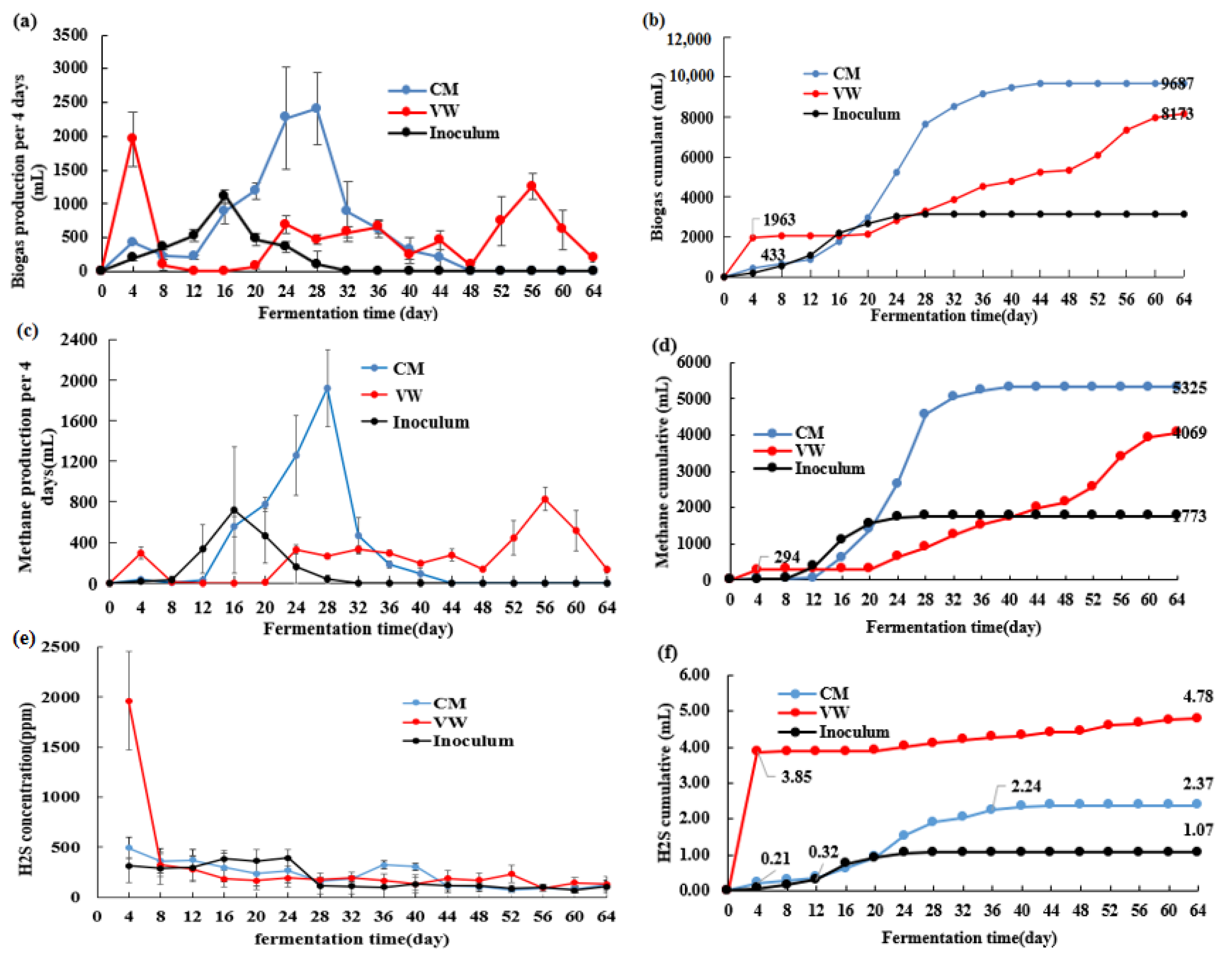
3.2.1. Biogas and CH4
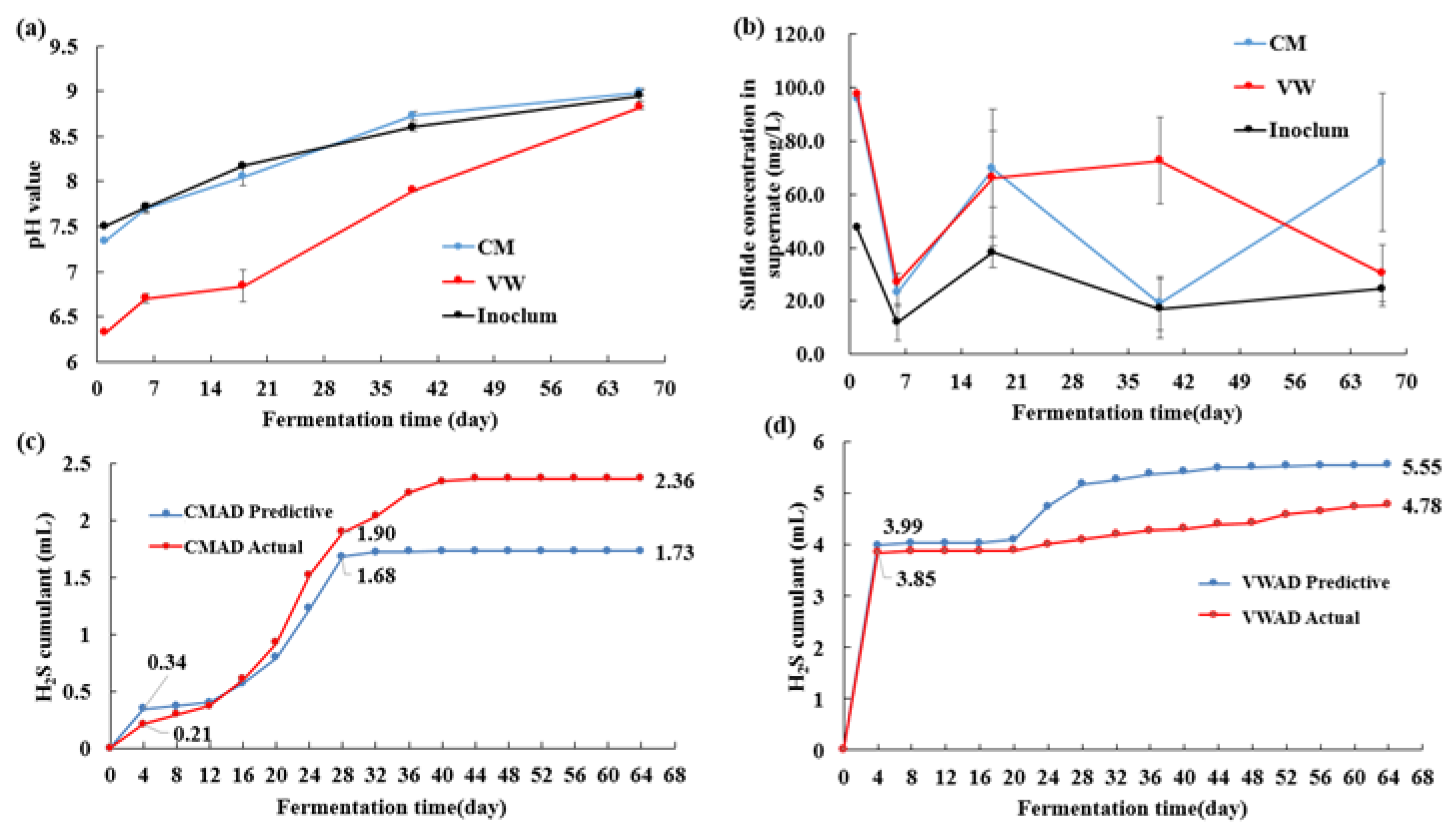
For CMAD, one biogas production peak appeared from day 12 to day 36 and the CH4 content of 45% on day 12 increased to 75% on day 32, with an average of 54.9% (Figure 2a–d and Table 2). The biogas production potential of CM was 314 m3/t (TS) (Table 2).
For VWAD, two biogas production peaks appeared (Figure 2a). The first one was observed on day 1, whereas the second peak was observed on day 52 and disappeared on day 60 (Figure 2a,b). Due to acidification (Figure 3a), the content of CH4 fell to less than 5% on day 1, following which it grew from 45% on day 20 to 70% on day 60 (Figure 2c,d). In addition, the content of H2 on day 1 was 30%, following which it declined to 0.5% after day 2. Therefore, the biogas’s average CH4 content was calculated to be 49.7% (Table 2). The biogas production potential of VW was 240 m3/t (TS) (Table 2).
The inoculum generated small amounts of biogas (Figure 2a–d), indicating the incomplete digestion of organic matter prior to measurements.
Based on the analysis above, the fermentation time of CMAD was shorter than that of VWAD, and the biogas production potential and CH4 content of CM were higher than those of VW.

3.2.2. H2S Emission

H2S concentrations for CMAD were between 156 and 492 ppm from day 1 to day 42, and there was a decline in the final concentrations to 72–112 ppm between days 46 and 67 (Figure 2e). The average concentration and production potential of H2S were calculated as 198 ± 79 ppm and 90 ± 37 g/t (TS), respectively (Table 2). Small amounts of H2S were produced at day 1, and most H2S was produced when the CH4 production peak appeared between day 12 and 36 (Figure 2a,c,e), which means the production of H2S was synchronous to that of CH4.
A general declining trend of H2S concentrations in VWAD was evident, with a particularly pronounced decline from 1960 ppm on day 1 to 280 ppm on day 4, with the final concentrations reaching 132–230 ppm between days 8 and 67 (Figure 2e). The H2S average concentration and production potential were calculated to be 738 ± 210 ppm and 288 ± 87 g/t (TS), respectively (see Table 2). On day 1, 80% of the H2S was produced, whereas 20% was produced during days 2 and 67 (Figure 2e). This result was similar to those of previous studies on anaerobic digestion of food waste. For example, H2S concentrations were measured within full-scale AD at 600–1500 ppm by Kang et al. [21] and Cen et al. [22].
H2S concentrations of the inoculum control were 112–311 ppm at the peak biogas production time (days 1 to 28). There was a subsequent decline in concentrations to 10 ppm on day 32, following which they stabilized at a light concentration between days 36 and 67.
The results showed that 80% of H2S was released during the CH4 yield peak in CMAD, and the production of H2S was synchronous to that of CH4. For VWAD, the majority of the production of H2S occurred during the initial fermentation stage, and the peak production times of H2S and CH4 were not synchronous. The average H2S concentrations in CMAD were substantially lower than those in VWAD, and the H2S production potential of CM was substantially lower than that of VW.

3.3. The Relationship between H2S, Sulfide, and pH

For CMAD, the pH increased gradually from 7.3 on day 0 to 8.9 on day 67 (Figure 3a). The supernatant sulfide concentration dropped dramatically from 95 mg/L on day 0 to 23 mg/L on day 6, following which it declined to 69 mg/L on day 17, and then fell to 19 mg/L on day 39, and grew again to 71 mg/L on day 67. The results of present study showed that about 1/25 of the supernatant sulfide in CMAD can be transformed into soluble sulfide.
Based on the pH values and the soluble sulfide concentration mentioned in the last paragraph, and using the sulfide equilibrium equations Equations (1)–(3), H2S production can be estimated. Figure 3c shows the estimated values of H2S production. In general, there was consensus between the predicted and measured values. The equilibrium model in particular predicted 88% of H2S from day 1 to 28; one-variable linear regression analysis showed R2 was 0.718 between actual value and predicted value from day 1 to day 68. It is worth noting that the sulfur in H2S only accounted for 1.8% of the total sulfide, i.e., only a small amount of sulfide in the liquor phase was transferred to biogas in CMAD. Different to our study model, Peu et al.’s [9] study showed that the H2S emission model in food waste AD was established based on ratio of sulfur and carbon, but this study did not provide an accurate proportion of sulfur’s different chemical forms.
For VWAD, there was a sharp decline in pH from 7.5 on day 0 to 6.3 on day 1, following which there was an increase from 6.7 on day 6 to 8.6 on day 67 (Figure 3a). The supernatant sulfide concentration fell dramatically from 97 mg/L on day 0 to 27 mg/L on day 6, following which it declined and stabilized at 66–72 mg/L between day 17 and 39 and decreased again to 30 mg/L on day 67. According to Table 1 and the TS ratio of VW to inoculum (1:2), the sulfide concentration of VWAD was 329 mg/L; thus, the proportion of the supernatant sulfide in relation to the total sulfide was between 8.2 and 29.4%. This result is similar to Belle et al.’s study [23]: their research found that the concentration of H2S in the biogas peaked at 3300 ppm on the first day of fermentation, while the pH dropped to 6.8; however, by the sixth day, the concentration of H2S dropped by 1300 ppm, while the pH increased to 7.5.
Based on the pH values and soluble sulfide concentration from last paragraph, using Equations (1)–(3), the H2S production can be estimated. Figure 3d shows that the predicted and measured values were similar, with 97% of H2S on day 1 predicted by sulfide ion equilibrium model; one-variable linear regression analysis showed R2 was 0.973 between the actual value and predicted value from day 1 to day 68. This result indicated that the majority of H2S produced on day 1 was a result of the high supernatant sulfide concentration due to the acidification of the system and the rapid production of biogas. It is worth noting that the sulfur of H2S accounted for only 3.6% of the total sulfide, i.e., only a small amount of sulfide in the liquor phase was transferred to biogas in CMAD and VWAD.
Based on the analysis above, there were very high concentrations of sulfide in CMAD and VWAD, and only a small amount of sulfide in the liquor phase was transferred to biogas. The characteristics of H2S production between CMAD and VWAD differed, but the sulfide ion equilibrium mode could accurately predict the H2S production process in AD with these two materials. The rate of biogas production and pH were the key factors for the release of H2S. The emissions of H2S observed on day 1 were not the result of biochemical processes, but rather physical and chemical processes.

3.4. Microbial Community Structure and Function

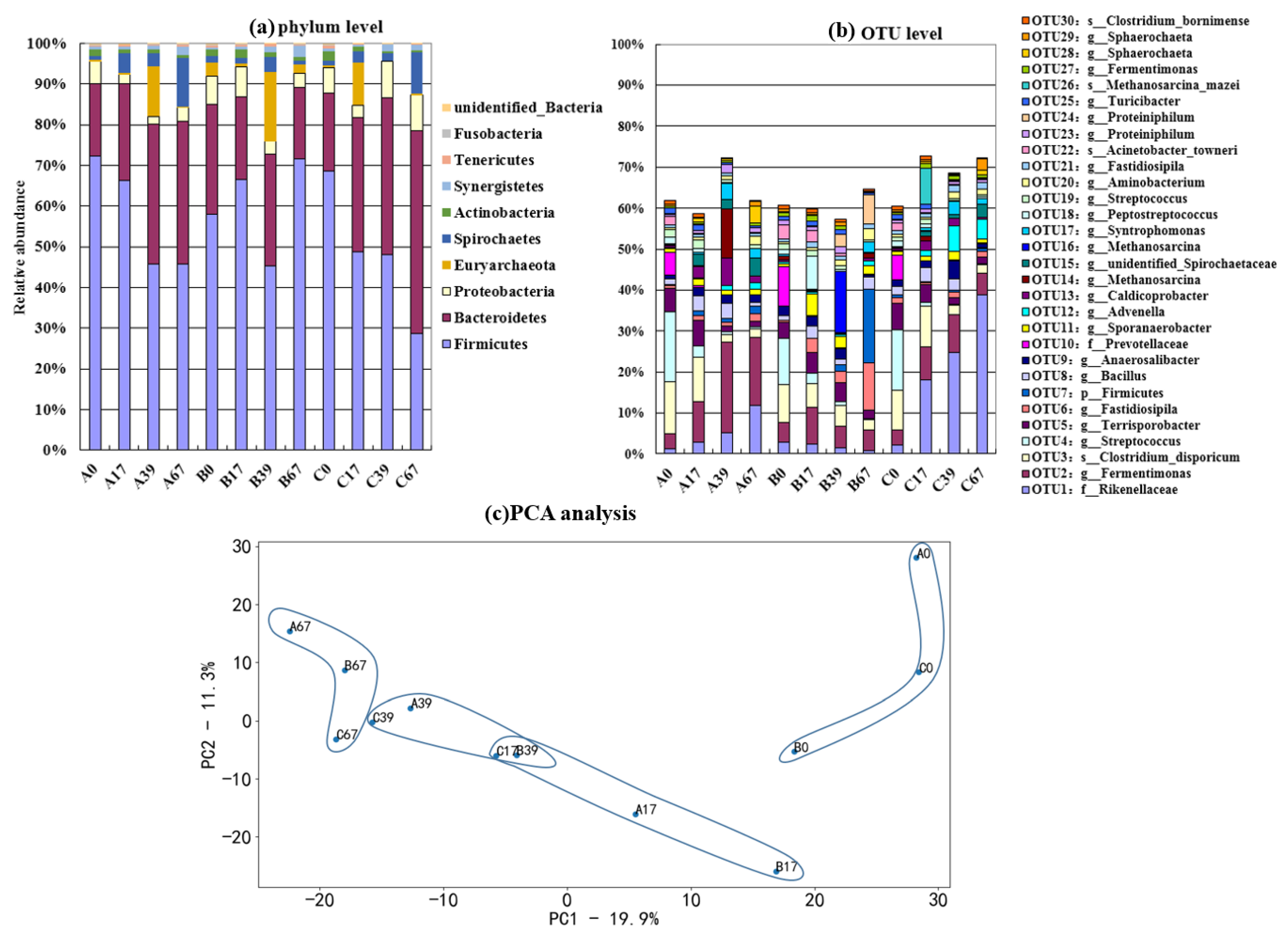
3.4.1. Microbial Community Structure at Phylum and OTUs Levels

As can be seen from Figure 3a, no matter CMAD or VWAD, the main microbial groups were Firmicutes, Bacteroidetes, Proteobacteria, and Euryarchaeota at the phylum level; these four phyla accounted for about 95% of the total microbes.
For CMAD (see Figure 4a,b), the abundance of Firmicutes, which contained genera (such as Clostridium) which can hydrolyze cellulose and hemicellulose [24,25], accounted for 72% at the initial period, then gradually declined by 47% at 39 d; it reamined stable until 67 d. The abundance of Bacteroidetes, which contains genera (such as Galbibacter) which can ferment glucose and produce H2/acetate [26], gradually increased from 18% at 0 d to 33% at 39 d; it remained at this level until 67 d. The abundance of Proteobacteria, which contains genera (such as Desulfomicrobium) which can reduce sulfate [27], was 7%, fell to 2% at 17 d, and was between 1.5 and 2.5% at from 39d to 67d. The abundance of Euryarchaeota, which contains genera (such as Methanosarsina, Methanobrevibacter) which can produce methane [28,29], was less than 1% at first 17 days, increased to 12% at 39 d, and then gradually decreased to 2% at 67 d. It is worth noting that the characteristics of the microbial community in the inoculum are similar to that of CM.
For VWAD (see Figure 4a,b), the abundance of Firmicutes was between 60 and 68% at a high abundance level before 17 d, indicating that Firmicutes was relatively adaptable to the acidic environment (pH = 6.5); it dropped to 47% at 39 d and was back to 71% at 67 d. The abundance of Bacteroidetes did not change much between 18 and 25% over the whole fermentation process. The abundance of Euryarchaeota was 6~7% before 17 d and decreased to 3% between 39 and 67 d. The abundance of Euryarchaeota decreased from 2% at the beginning to 0.2% at 17 d, increased to 18% in the early stage of the methane production peak (39 d), and decreased to 1% at the end of the CH4 production peak (67 d).

3.4.2. Principal Component Analysis (PCA)

As can be seen from Figure 4b, during the intial stages of fermentation, the microbial community structures of A0, B0, and C0 were similar because the raw material and inoculum were mixed at the starting time and the microorganisms were mainly from the inoculum. By day 17, the community structures of A17, B17, and C17 were different: A17 was in the slow production phase of CH4 (pH: 7.4), B17 was in the acidification phase (pH: 6.5), and C17 was at the peak production period of CH4 (pH: 7.8). After 39 days of fermentation, the microbial community structures between A39, B39, and C39 were similar because the 39th day is the peak period or close to the peak period of CH4 production for different fermented raw materials. In the final stage of fermentation, the microbial community structures between A67, B67, and C67 were similar because the fermentation of each raw material was already in the later and organic matter was not available, the microorganisms were lacking a food source. In summary, the influence of the fermentation period on the microbial community was greater than that of the type of raw material.

3.4.3. Microbial Community Function Concerning Sulfide Metabolism

For the reduction in sulfate in CMAD, the abundance of the gene concerning sulfate reduction was relatively stable and low, between 0.01 and 0.07% during the whole process (Table 3); i.e., sulfate reduction occurred from the start to the end of the experiment. Thus, the biochemical process of the conversion of sulfate in CM to sulfide/H2S was slow and continuous. For protein decomposition in CMAD, the genes linked to fermentation and playing roles in anaerobic acidification and decomposition of macromolecular organic matter (e.g., amino acids) exhibited high abundances between 22.8 and 30.5% before day 17 (Table 3). They subsequently fell to 6.27–10.28% after day 39. Thus, these genes were identified as important for the transformation of organic sulfur (such as protein) to sulfide between days 0 and 17.
For sulfate reduction in VWAD, the abundance of sulfate reduction genes was relatively stable and low, between 0.01 and 0.05% during the process (Table 3), indicating that sulfate reduction occurred from the start to the end of the experiment. Thus, sulfate in VW (high sulfate) was slowly and continuously converted to sulfide/H2S, which provides important evidence for the fact that the large production of H2S on the first day was caused by the sulfide reaching chemical equilibrium and not by sulfate reduction. Similarly, another study showed that the AD of food waste can convert sulfate to sulfide/H2S in a long-term biochemical process and that large amounts of H2S were produced on the first day by the sulfide ion equilibrium [13,30]. For protein decomposition in VWAD, the genes linked to fermentation and which play roles in the anaerobic acidification and decomposition of macromolecular organic matter (e.g., amino acids) exhibited a high abundance, between 22.7 and 22.8%, before day 17 (Table 3). Subsequently, they fell to 8.82–9.45% after day 39. Therefore, these genes are important for the transformation of S-protein to S-sulfide between days 0 and 17. This indicates that the large production of H2S on the first day was not caused by protein decomposition. Another study showed that food waste AD can convert protein to sulfide/H2S in a long-term biochemical process [13,30].
Generally, independent of focusing on CMAD or VWAD, the abundance of sulfate reduction bacteria (SRB) and microbes concerning organosulfur compounds (such as amino acids and protein) fermentation were stable in the fermentation process: the abundance of SRB was 0.01~0.07%, while that concerning organosulfur compounds fermentation was 22.8~30.5%.

4. Conclusions

In this study, H2S production characteristics of CMAD and VWAD were observed. The H2S production potential of CM was substantially lower than that of VW because it was easier to produce a large number of organic acids from VW than from CM. The rapid production of biogas and fermentation acidification were important reasons for the release of H2S at the start of CMAD. The sulfide equilibrium model in AD was capable of predicting H2S production in both CMAD and VWAD. Furthermore, the abundance of sulfate reduction bacteria (SRB) and microbes concerning the fermentation of organosulfuric compounds were stable in the fermentation process: the abundance of SRB was 0.01~0.07%, while that concerning the fermentation of organosulfuric compounds was 22.8~30.5%. This study indicated that the H2S concentration of CMAD biogas was more than five times that of VWAD because CM is alkalescent and VW is acidic; therefore, the potential strategy for controlling H2S in situ in CMAD is different than in VWAD. In the future, it is important to systematically compare H2S emission differences between acidic material (such as vegetable waste and food waste) and alkaline material (such as pig manure) in AD.

Supplementary Materials

The following supporting information can be downloaded at: https://www.mdpi.com/article/10.3390/fermentation9020169/s1, File S1: Calculation process of the equilibrium from sulfide to H2S in the liquid phase.

Author Contributions

Writing—original draft preparation, G.T.; data curation, M.Y.; writing—review and editing, J.X. All authors have read and agreed to the published version of the manuscript.

Funding

This research was supported by the Special Research Fund of Natural Science of Guizhou University (Grant No. X2020085), the Major Science and Technology Program for Water Pollution Control and Treatment of China (Grant No. 2011ZX07301-003), and the National Natural Science Foundation of China (Grant No. 51378286).

Institutional Review Board Statement

Not applicable.

Informed Consent Statement

Not applicable.

Data Availability Statement

Not applicable.

Conflicts of Interest

The authors declare that they have no known competing financial interest or personal relationships that could have appeared to influence the work reported in this paper.

References

  1. Du, P.; Han, X.; Gao, J.; Chen, Q.; Li, Y. Potential Analysis on High Efficient Utilization of Waste Vegetable Resources in China. China Veg. 2015, 7, 15–20. [Google Scholar]
  2. Peng, X.; Fu, J.; Li, C.; Tang, J. Research Advance and Prospect on Vermicomposting of Chicken Excrement. China Poult. 2018, 40, 1–7. [Google Scholar]
  3. Chen, Y.C.; Higgins, M.J.; Beightol, S.M.; Murthy, S.N.; Toffey, W.E. Anaerobically digested biosolids odor generation and pathogen indicator regrowth after dewatering. Water Res. 2011, 45, 2616–2626. [Google Scholar] [CrossRef] [PubMed]
  4. Zhang, Y.; Zhang, L.; Yu, N.; Guo, B.; Liu, Y. Enhancing the resistance to H2S toxicity during anaerobic digestion of low-strength wastewater through granular activated carbon (GAC) addition. J. Hazard. Mater. 2022, 430, 128473. [Google Scholar] [CrossRef]
  5. Yang, L.; Lamont, L.D.; Sedbrook, J.C.; Heller, N.J.; Kopsell, D.E. Anaerobic Digestion of Cereal Rye Cover Crop. Fermentation 2022, 8, 617. [Google Scholar] [CrossRef]
  6. Fu, Q.; Liu, X.; He, D.; Li, X.; Li, C.; Du, M.; Wang, Y.; Long, S.; Wang, D. Rhamnolipid increases H2S generation from waste activated sludge anaerobic fermentation: An overlooked concern. Water Res. 2022, 221, 118742. [Google Scholar] [CrossRef] [PubMed]
  7. Akgul, D.; Abbott, T.; Eskicioglu, C. Assessing iron and aluminum-based coagulants for odour and pathogen reductions in sludge digesters and enhanced digestate dewaterability. Sci. Total Environ. 2017, 598, 881. [Google Scholar] [CrossRef] [PubMed]
  8. Orzi, V.; Cadena, E.; D’Imporzano, G.; Artola, A.; Davoli, E.; Crivelli, M. Potential odour emission measurement in organic fraction of municipal solid waste during anaerobic digestion: Relationship with process and biological stability parameters. Bioresour. Technol. 2010, 101, 7330–7337. [Google Scholar] [CrossRef]
  9. Peu, P.; Picard, S.; Diara, A.; Girault, R.; Béline, F.; Bridoux, G.; Dabert, P. Prediction of hydrogen sulphide production during anaerobic digestion of organic substrates. Bioresour. Technol. 2012, 121, 419–424. [Google Scholar] [CrossRef]
  10. Díaz, I.; Ramos, I.; Fdz-Polanco, M. Economic analysis of microaerobic removal of H2S from biogas in full-scale sludge digesters. Bioresour. Technol. 2015, 192, 280–286. [Google Scholar] [CrossRef]
  11. Zeng, Q.; Hao, T.; Sun, B.; Luo, J.; Chen, G.; Crittenden, J.C. Electrochemical Pretreatment for Sludge Sulfide Control without Chemical Dosing: A Mechanistic Study. Environ. Sci. Technol. 2019, 53, 14559–14567. [Google Scholar] [CrossRef]
  12. Dai, X.; Hu, C.; Zhang, D.; Chen, Y. A new method for the simultaneous enhancement of methane yield and reduction of hydrogen sulfide production in the anaerobic digestion of waste activated sludge. Bioresour. Technol. 2017, 243, 914–921. [Google Scholar] [CrossRef] [PubMed]
  13. Tian, G.; Xi, J.; Yeung, M.; Ren, G. Characteristics and mechanisms of H2S production in anaerobic digestion of food waste. Sci. Total Environ. 2020, 724, 137977. [Google Scholar] [CrossRef] [PubMed]
  14. Berg, J.; Brandt, K.K.; Al-Soud, W.A.; Holm, P.E.; Hansen, L.H.; Sørensen, S.J. Selection for Cu-tolerant bacterial communities with altered composition, but unaltered richness, via long-term Cu exposure. Appl. Environ. Microbiol. 2012, 78, 7438–7446. [Google Scholar] [CrossRef]
  15. Bolyen, E.; Rideout, J.R.; Dillon, M.R.; Bokulich, N.A.; Abnet, C.C.; Al-Ghalith, G.A.; Bai, Y. Reproducible, interactive, scalable and extensible microbiome data science using QIIME 2. Nat. Biotechnol. 2019, 37, 852–857. [Google Scholar] [CrossRef] [PubMed]
  16. Martin, M. Cutadapt removes adapter sequences from high-throughput sequencing reads. EMBnet. J. 2011, 17, 10–12. [Google Scholar] [CrossRef]
  17. Callahan, B.J.; Mcmurdie, P.J.; Rosen, M.J.; Han, A.W.; Johnson, A.J.A.; Holmes, S.P. Dada2: High-resolution sample inference from illumina amplicon data. Nat. Methods 2016, 13, 581–583. [Google Scholar] [CrossRef]
  18. Glick, M.; Klon, A.E.; Acklin, P.; Davies, J.W. Enrichment of extremely noisy high-throughput screening data using a naive Bayes classifier. J. Biomol. Screen. 2004, 9, 32–36. [Google Scholar] [CrossRef]
  19. Louca, S.; Parfrey, L.W.; Doebeli, M. Decoupling function and taxonomy in the global ocean microbiome. Science 2016, 353, 1272–1277. [Google Scholar] [CrossRef]
  20. Rognes, T.; Flouri, T.; Nichols, B.; Quince, C.; Mahé, F. VSEARCH: A versatile open source tool for metagenomics. Peer J. 2016, 4, e2584. [Google Scholar] [CrossRef]
  21. Kang, J.W.; Jeong, C.M.; Kim, N.J.; Kim, M.I.; Chang, H.N. On-site removal of H2S from biogas produced by food waste using an aerobic sludge biofilter for steam reforming processing. Biotechnol. Bioprocess Eng. 2010, 15, 505–511. [Google Scholar] [CrossRef]
  22. Cen, R.; Chen, R.; Pu, T.; Huang, C.; He, T.; Tian, G. Feeding controls H2S production in situ in high solid anaerobic digestion. Bioresour. Bioprocess. 2022, 9, 79. [Google Scholar]
  23. Belle, A.J.; Lansing, S.; Mulbry, W.; Weil, R.R. Methane and hydrogen sulfide production during co-digestion of forage radish and dairy manure. Biomass Bioenergy 2015, 80, 44–51. [Google Scholar] [CrossRef]
  24. Fonknechten, N.; Chaussonnerie, S.; Tricot, S.; Lajus, A.; Andreesen, J.R.; Perchat, N.; Kreimeyer, A. Clostridium sticklandii, a specialist in amino acid degradation: Revisiting its metabolism through its genome sequence. BMC Genom. 2010, 11, 555. [Google Scholar] [CrossRef]
  25. Nathani, N.M.; Duggirala, S.M.; Bhatt, V.D.; Patel, A.K.; Kothari, R.K.; Joshi, C.G. Correlation between genomic analyses with metatranscriptomic study reveals various functional pathways of Clostridium sartagoforme AAU1, a buffalo rumen isolate. J. Appl. Anim. Res. 2016, 44, 498–507. [Google Scholar] [CrossRef]
  26. Zhilina, T.N.; Appel, R.; Probian, C.; Brossa, E.L.; Harder, J.; Widdel, F.; Zavarzin, G.A. Alkaliflexus imshenetskii gen. nov. sp. nov., a new alkaliphilic gliding carbohydrate-fermenting bacterium with propionate formation from a soda lake. Arch. Microbiol. 2004, 182, 244–253. [Google Scholar] [CrossRef]
  27. Li, Y.; Jin, Y.; Li, H.; Borrion, A.; Yu, Z.; Li, J. Kinetic studies on organic degradation and its impacts on improving methane production during anaerobic digestion of food waste. Appl. Energy 2018, 213, 136–147. [Google Scholar] [CrossRef]
  28. Hiroyuki, M.; Masateru, N.; Yosuke, K. Isolation, Characterization and Physiology of a New Formate-assimilable Methanogenic Strain (A2). J. Agric. Chem. Soc. Jpn. 2014, 38, 1628–1638. [Google Scholar]
  29. Morii, H.; Nishihara, M.; Koga, Y. Isolation, characterization and physiology of a new formate-assimilable methanogenic strain (A2) of Methanobrevibacter arboriphilus. Agric. Biol. Chem. 1983, 47, 2781–2789. [Google Scholar] [CrossRef]
  30. Khanthongthip, P.; Yagci, N.; Orhon, D.; Novak, J. Generation and fate of volatile organic sulfur compounds during anaerobic digestion of waste activated sludge. Desalin. Water Treat. 2021, 215, 279–287. [Google Scholar] [CrossRef]
Figure 1. Schematic of the batch biogas fermentation system (1. The volume of saturated salt water is 95% of the volume of the biogas storage bottle at fermentation starting time, and the water is pressured to metering bottle by biogas resulted from chicken manure (or vegetable waste) AD. Stirring is not performed during the anaerobic process. 2. The volume of biogas has been measured according to the volume of saturated salt water in the metering bottle, then, a sample of biogas was taken from sampling port. 3. Fifty-milliliter aluminum foil bags were used to collect biogas containing H2S from the sampling port for testing the biogas components).
Fermentation 09 00169 g001
Figure 2. Characteristics of biogas, CH4, and H2S production in CMAD and VWAD: (a) biogas yield every 4 days; (b) biogas cumulative; (c) CH4 production every 4 days; (d) methane cumulative; (e) H2S concentration; (f) cumulative H2S.
Fermentation 09 00169 g002
Figure 3. The estimation of H2S based on sulfide ionization equilibrium model and the Henry theorem: (a) pH value; (b) sulfide concentration in supernate; (c) predicted and actual values of H2S cumulative in CMAD; (d) predictive and actual values of cumulative H2S in VWAD.
Fermentation 09 00169 g003
Figure 4. The microbial community structure at the phylum level (a) and species (b) and PCA analysis (c). Note: (a) the top 30 most abundant OTUs are shown; (b) A0, B0, and C0 represent the CMAD, VWAD, and day 0 samples of inoculum, respectively.
Fermentation 09 00169 g004
Table 1. Characteristics of chicken manure (CM), vegetable waste (VW), and inoculum.
ItemsCMVWInoculum
TS (%)27.1 ± 1.77.2 ± 0.45.2 ± 0.3
VS (%) (dry basis)72.3 ± 2.587.5 ± 1.556.5 ± 2.2
Ash (%) (dry basis)27.7 ± 1.612.5 ± 2.243.5 ± 2.1
ORP (mV)−327 ± 19152 ± 15−279 ± 12
DO (mg/L)0.15 ± 0.107.37 ± 10.16 ± 0.11
pH7.37 ± 0.165.08 ± 0.228.5 ± 0.10
Protein (%) (dry basis)3.9 ± 0.511.4 ± 1.31.5 ± 0.15
S-sulfide (mg/kg) (dry basis)2566 ± 354264 ± 148750 ± 279
S-sulfate (mg/kg) (dry basis)1922 ± 2721527 ± 220653 ± 37
S-total (mg/kg) (dry basis)7509 ± 4803152 ± 3179576 ± 643
S-protein (mg/kg) (dry basis)388113919
Table 2. Production potential and concentration of biogas and H2S.
CMVW
Biogas production potential (m3/ton (TS))314 + 92240 + 78
Average methane content (%)54.9 + 3.149.7 + 2.2
H2S production potential (g/ton (TS))90 ± 37288 ± 87
Average H2S concentration (ppm)198 + 79738 ± 210
Table 3. Abundance (%) of genes with a metabolism function based on FAPROTAX predictions.
Functional GroupsChicken Manure AD (%)Vegetable Waste AD (%)Inoculum (%)
A0A17A399A67B0B17B399B67C0C17C39C67
Methanogenesis0.210.266.970.201.700.397.791.540.265.340.090.34
Sulfate respiration0.030.070.010.040.030.040.010.010.050.040.060.03
Sulfur respiration0.480.950.641.120.432.831.281.560.460.511.620.92
Sulfite respiration0.020.060.010.030.030.020.010.010.030.040.050.03
Thiosulfate respiration0.010.020.010.010.020.020.010.000.020.020.010.01
Respiration of sulfur compounds0.521.050.661.180.502.891.301.570.540.571.690.96
Dark sulfide oxidation0.000.000.000.060.010.010.010.010.010.000.040.06
Dark sulfur oxidation0.000.000.000.060.000.010.010.010.010.000.040.05
Dark thiosulfate oxidation0.000.000.000.060.000.010.010.010.010.000.050.06
Dark oxidation_of_sulfur_compounds0.000.000.000.060.010.010.010.0130.010.000.040.06
Fermentation30.0522.856.2710.2822.2722.389.458.8227.1512.538.828.013
Note: A0, B0, and C0 represent the chicken manure AD, vegetable waste AD, and day 0 samples of inoculum, respectively.
Disclaimer/Publisher’s Note: The statements, opinions and data contained in all publications are solely those of the individual author(s) and contributor(s) and not of MDPI and/or the editor(s). MDPI and/or the editor(s) disclaim responsibility for any injury to people or property resulting from any ideas, methods, instructions or products referred to in the content.

