Article

Modeling and Simulation of Batch Sugarcane Alcoholic Fermentation Using the Metabolic Model

by
Renam Luis Acorsi
,
Matheus Yuri Gritzenco De Giovanni
,
José Eduardo Olivo
and
Cid Marcos Gonçalves Andrade
*
Departamento de Engenharia Química, Universidade Estadual de Maringá, Av. Colombo 5790, Maringá 87020-900, PR, Brazil
*
Author to whom correspondence should be addressed.
Fermentation 2022, 8(2), 82; https://doi.org/10.3390/fermentation8020082
Submission received: 31 January 2022 / Revised: 9 February 2022 / Accepted: 9 February 2022 / Published: 16 February 2022
(This article belongs to the Section Fermentation Process Design)

Abstract

:
The present work sought to implement a model different from the more traditional ones for the fermentation process of ethanol production by the action of the fungus Saccharomyces cerevisiae, using a relevant metabolic network based on the glycolytic Embden–Meyerhof–Parnas route, also called “EMP”. We developed two models to represent this phenomenon. In the first model, we used the simple and unbranched EMP route, with a constant concentration of microorganisms throughout the process and glucose as the whole substrate. We called this first model “SR”, regarding the Portuguese name “sem ramificações”, which means “no branches”. We developed the second model by simply adding some branches to the SR model. We called this model “CR”, regarding the Portuguese name “com ramificações”, which means “with branches”. Both models were implemented in MATLABTM software considering a constant temperature equal to 32 °C, similar to that practiced in sugar and ethanol plants, and a wide range of substrate concentrations, ranging from 30 to 100 g/L, and all the enzymes necessary for fermentation were already expressed in the cells so all the enzymes showed a constant concentration throughout the fermentation. The addition of common branches to the EMP route resulted in a considerable improvement in the results, especially predicting ethanol production closer to what we saw experimentally. Therefore, the results obtained are promising, making adjustments consistent with experimental data, meaning that all the models proposed here are a good basis for the development of future metabolic models of discontinuous fermentative processes.

1. Introduction

A wide range of fermented products are still produced by batch or sequential batch processes using easily accessible raw materials. In the case of ethanol production, biofuel is of interest to compete with fossil fuels, since its use brings a reduction in the emission of harmful gases, such as SOx and NOx. This is similar to the use of one of the most widely used processes in the production of this alcohol, the Melle-Boinot process, a form of fed-batch fermentation developed by Fermin Boinot, in the town of Melle, located in the Nouvelle-Aquitaine region of France, in the first half of the 20th century. Furthermore, in the production of ethanol, the yeast Saccharomyces cerevisiae is the most used microorganism, even if other microorganisms have a better potential in laboratory situations, such as the bacterium Zymomonas mobilis [1,2,3,4].
Due to the importance of this type of process, from the second half of the 20th century, a series of works seeking to understand these interactions began to be developed, especially after Gaden [5], who developed an empirical analysis (black box) of batch fermentation processes, verifying whether it was possible to associate the production of a metabolite with cell growth or not. This relatively simple approach had good results, despite ignoring a large part of the interactions that occur inside the cells. Because of this, numerous works were developed based on the work of Gaden and the kinetic model of Monod, making additions that sought to insert any metabolic knowledge.
Among the models that began seeking to insert these metabolic details, we can mention the model developed by Sonnleitner and Käppeli [6], developed based on a quasi-ideal Monod kinetic model. In such a model, Sonnleitner and Käppeli simplified the relevant metabolism into three stoichiometric relationships: two containing purely oxidative relationships, and one reductive. Furthermore, this model already considered the possibility of alcoholic fermentation not being fueled by a single substrate: it considered the possibility of multiple substrates, such as the possibility of ethanol being used by Saccharomyces cerevisiae as a carbon source. Despite the relevant results achieved in such a model, it still considered the great metabolic complexity in an extremely simplified way.
In addition to the model by Sonnleitner and Käppeli [6], several other relevant models for alcoholic fermentation were developed in a black box or with the addition of some metabolic details. Among such models, we can cite the work of Birol et al. [7], Kostov et al. [8], Sainz et al. [9], and Freitas et al. [10]. The works by Birol et al. [7] and Kostov et al. [8] have the merit of analyzing a large number of black box models for alcoholic fermentation, highlighting the Monod, Andrews, Naock, and Hinshelwood models. Fermentation processes conducted in batch and fed-batch form generate a considerably complex dynamic interaction between microorganisms and the environment around them, as studied by Freitas et al. [10] using genetic algorithms, differential evolution, and real-time dynamic optimization. These interactions have been generally studied and well analyzed in the form of black box analyses for some decades, as highlighted by Sainz et al. [9], but they fail to consider that each of the cells of a microorganism is capable of carrying out hundreds of reactions simultaneously. It was fair to the model proposed by Sainz et al. [9] that such interactions began to be considered. Each of these reactions is extremely well controlled by the action of substances that generate the expression of or inhibit very specific biocatalysts—enzymes [11,12].
Among the most important metabolic routes for numerous fermentative processes, we can mention the Embden–Meyerhof–Parnas route, or the EMP route. Completely described in the 1940s, the EMP pathway is present in a large number of organisms and describes a series of spontaneous reactions that convert glucose to pyruvate. The pyruvate generated in this sequence can be converted into a wide range of other substances, including ethanol, which can be produced under anaerobic conditions by reducing pyruvate [11,13,14,15].
Considering the importance of ethanol in the current economic and environmental scenario, as well as the development of models that are more faithful to reality, the present work sought to model a batch alcoholic fermentation process. We used kinetic equations derived from the EMP route of Saccharomyces cerevisiae, considering substrate concentrations lower than those used industrially to avoid the appearance of significant inhibitory effects. The production of ethanol still needs further clarification at the metabolic level. Thus, we propose two distinct models: the SR model, built only with the reactions present in the EMP route followed by alcoholic fermentation, and the CR model, which consists of using the SR model as a basis, adding the ramifications of trehalose, glycerol, succinate, and acetate. Furthermore, the development of models based on as much metabolic information as possible can benefit countless other industrial sectors besides sugar and alcohol: an understanding of the behavior of possible ramifications is something that would greatly benefit the food and pharmaceutical industries, for example. In the case of the food industry, this knowledge would make better control of the processes and the selection and development of new strains of microorganisms possible, making it possible to obtain larger amounts of specific substances, especially those involved in aromas and flavors.

2. Method and Experimental Procedures

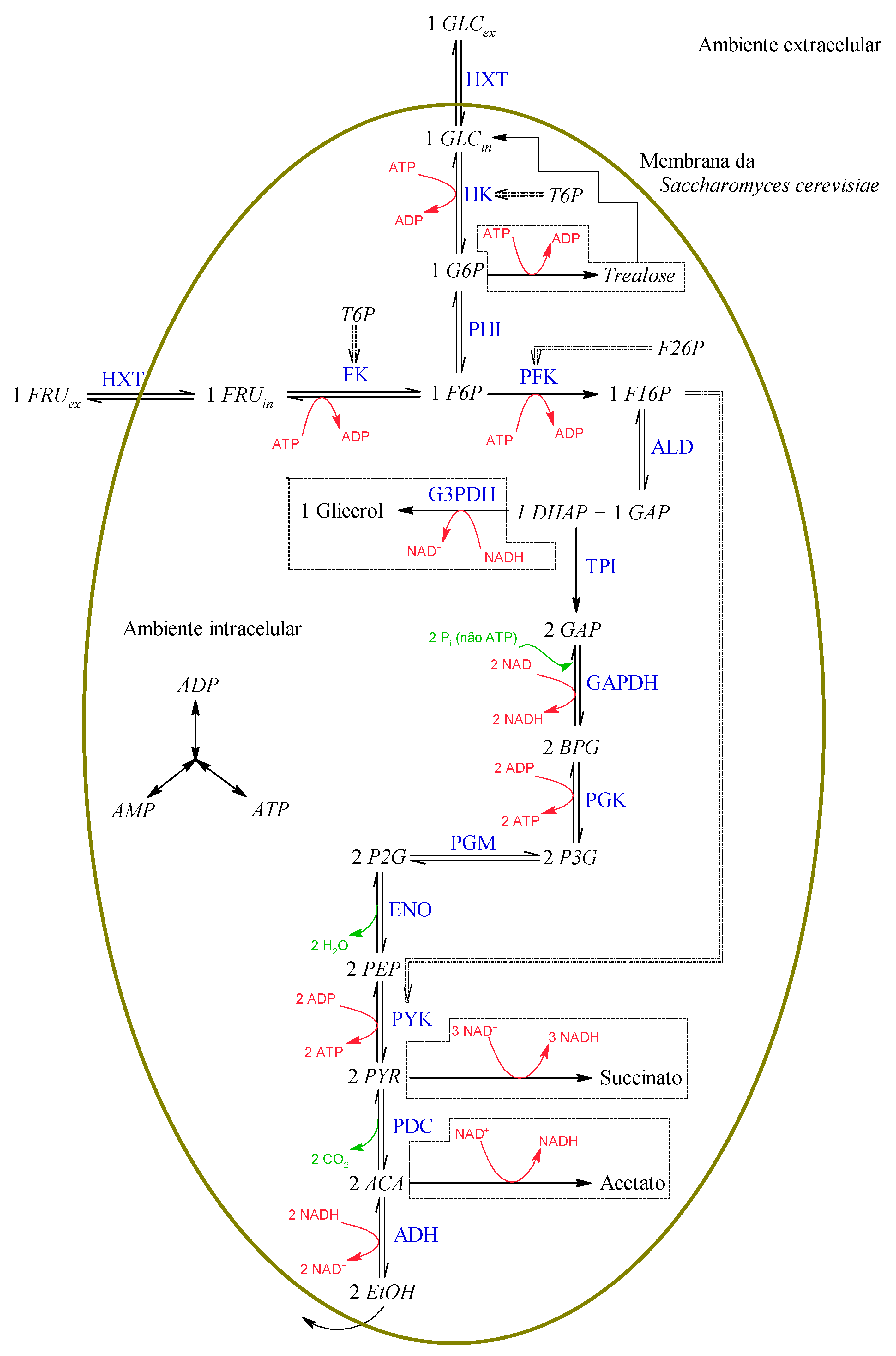
Figure 1 below shows the sequence of reactions selected for the composition of the model. In short, there are the transport of the substrate from the extracellular environment to the intracellular environment, the EMP route, and alcoholic fermentation. Additionally, highlighted are the enzymes responsible for each of the reactions, in blue; products or resulting secondary reagents, in green; and the intracellular energy molecules ADP, ATP, NAD+, and NADH, in red. A list of symbols and meanings is available in the end of this paper.
In Figure 1, there is the existence of two substrates, glucose (GLCex) and fructose (FRUex), where the “ex” subscript indicates that these substances are found in an extracellular environment. Even though the yeast metabolizes these two sugars and both are originally present in the raw material, used at the ratio of 52.5% glucose and 47.5% fructose, in this work, we assumed that the only substrate available is glucose for reasons of simplification. Furthermore, there is only one metabolic product of interest, ethanol, EtOH.
In addition to these substances, there is a series of intracellular metabolites: GLC in , ADP , ATP , TRE , FRU in , G 6 P , F 6 P , F 16 P , DHAP ,   GAP , GLY , P i , BPG , NAD , NADH , P 3 G , P 2 G , PEP , PYR , ACA , SUC , ACE , T 6 P , and F 26 P . Thus, starting from the sequence of metabolic reactions shown in Figure 1, we propose the following set of differential equations for such a model:
d G L C e x d t = v H X T , G
d E t O H d t = v A D H
d G L C i n d t = v H X T , G v H K 2 v T R E 1
d A T P d t = v P G K + v P Y K v H K v P F K 2 v T R E 2
d T R E d t = v T R E 2 v T R E 1
d G 6 P d t = v H K v P H I 2 v T R E 2
d F 6 P d t = v P H I v P F K
d F 16 P d t = v P F K v A L D
d D H A P d t = v A L D v G L Y v T P I
d G A P d t = v A L D v G A P D H + v T P I
d G L Y d t = v G L Y
d P i d t = v G A P D H
d B P G d t = v G A P D H v P G K
d N A D H d t = v A C E + v G A P D H + 3 v S U C v G L Y v A D H
d P 3 G d t = v P K G v P G M
d P 2 G d t = v P G M v E N O
d P E P d t = v E N O v P Y K
d P Y R d t = v P Y K v P D C 2 v S U C
d A C A d t = v P D C v A D H v A C E
d S U C d t = v S U C
d A C E d t = v A C E
The model generated from Equations (1)–(21) constitutes what will be called the CR model, that is, the most complete model that considers the existence of ramifications in the EMP route followed by alcoholic fermentation. On the other hand, the simplest model, called the SR model, is the model for which the velocities of Equations (5), (11), (20), and (21) will be equal to zero, that is, the SR model is the model where the EMP route and alcoholic fermentation occur directly and without deviations. Furthermore, as the focus of the present work is the development of a model for alcoholic fermentation, and cell reproduction in alcoholic fermentation in an anaerobic medium is low, we opted for the simplified use of kinetic relationships for cell growth, as will be discussed later.
A problem that may occur when using all these reactions in a metabolic model relates to the concentrations of energetic molecules, such as AMP, ADP, ATP, T6P, and NAD. These substances are used in numerous other reactions that occur in cell metabolism, being generated and consumed, thus maintaining such substances at approximately constant levels in healthy cells. Therefore, as chosen in the model proposed by van Eunen et al. [16], we decided to maintain the levels of these substances as constant in the present work. In addition to these substances, F26P is also another substance of importance in the metabolic network in question, but it is difficult to measure and ended up having its concentration considered as constant as well. In Table 1, we list the fixed concentrations for such substances.
In addition to constant concentrations, we need to employ a series of initial concentrations for the relevant metabolites in order to solve the model. The use of good initial values is essential for a good model response; however, finding practical values for the initial concentration of metabolites is complex. Teusink [17] and van Eunen [16] used a similar set of initial concentrations of substances, but some concentrations used by them were considerably high compared to the data presented in other works, such as Sato et al. [18], Ruoff et al. [19], Casei et al. [20], and Peeters et al. [21]. Thus, based on the data presented in such studies, we list the initial concentrations of metabolites in Table 2 below.
The importance of choosing the initial values used for solving the systems of differential equations found in the present work should be highlighted. The system of differential equations proposed to solve the problem treated in the present work consists of a set of stiff differential equations, which generates a highly nonlinear system of differential equations. That said, the initial conditions used in solving the problem are extremely important, since a set of initial values can easily lead to non-convergence of values or even to mathematically correct results that are unrealistic in practice. Thus, a search was carried out in other works in the literature for initial concentration values for the various substances found in the system proposed here, looking for those that produced more stable and biologically viable results. Therefore, a series of initial values for the substances was tested in the model proposed here, noticing three types of behaviors, used as groups. The first group of values included values of the initial concentration of certain metabolites, such as fructose-6-phosphate and pyruvate, which presented a very abrupt drop in concentrations in the initial periods of fermentation, generating instability in the resolution, including negative concentrations. The second group of values included initial values that presented the opposite behavior, with an abrupt growth, generating concentrations biologically impossible to see inside a cell—in the case of glucose-6-phosphate, fructose-1,6-bisphosphate, and trioses. The third group of values generated a more stable response consistent with data found in the literature.
The initial substrate concentration in the present work varied between 30 g/L, 75 g/L, and 100 g/L. Another point we considered in this type of modeling is related to the cell concentration. Under anaerobic conditions with low substrate concentrations, Saccharomyces cerevisiae does not reproduce as much as under aerobic conditions. This consideration makes it common for the cell concentration to be set as constant in such fermentation assays; however, as the cell concentration relates directly to the enzyme concentration, the consideration of a variable amount of cells certainly enriches the model. Therefore, in the present model, we considered the cell concentration to follow the Andrews and Noack model, a simple model derived from the Monod model that showed a good predictive capacity according to the work of Kostov et al. [8].
μ = 1 X d X d t = μ 0 [ S ] 1 + K S X S + S K i S
This Andrews and Noack model is a black box model, that is, it does not consider peculiarities regarding the fungus metabolism. The growth metabolism is extremely complex and not addressed in the present work. The purpose of inserting this growth model is just to add dynamic behavior to the cell concentration. Furthermore, the Andrews and Noack model takes into account a possible inhibitory effect on cell growth due to excess substrate in the culture medium, something important to take into account, since inhibitory effects on growth tend to appear even at lower levels of the substrate concentration.
With this, it is possible to start solving the system of equations. Both the kinetic equations and the parameters used are in the Appendix A and Appendix B. The values of the kinetic parameters for the action of the enzymes hexokinase (HK), phosphohexoisomerase (PHI), phosphofructokinase (PFK), fructose-bisphosphate aldolase (ALD), triose-phosphate isomerase (TPI), glyceraldehyde-3-phosphate dehydrogenase (GAPDH), bisphosphoglycerate mutase (PGK), phosphoglycerate mutase (PGM), enolase (ENO), pyruvatokinase (PYK), pyruvate decarboxylase (PDC), and alcohol dehydrogenase (ADH) were taken from Teusink et al. [22], Berthels et al. [23], van Eunen et al. [16], and Smallbone et al. [24].
For HXT, there is the limiting step of the fermentation process: that is, it is expected that this step presents a greater variety of possible values than the other steps. Thus, we carried out a manual search within a range of possible values for the kinetic constants, coming from the same works mentioned above. These constants are called apparent, as they vary with the initial conditions of the fermentation process, and the model proposed here does not aim to incorporate repression or expression terms into the behavior of proteins.
The models were validated using data from Acorsi et al. [25]. In the batch fermentation carried out in such works, the culture media used were prepared based on diluted final sugarcane honey and inverted at 50 °C with the addition of 1 mL of invertase solution for each 100 mL of the desired medium, where the enzyme solution contained 4 mg/mL of invertase. The raw material was provided by “Usina Santa Terezinha Iguatemi Unit” and collected directly from the output of the continuous honey centrifuge B, being the same raw material that supplies the plant’s fermentation vats.
We carried out fermentation tests from 30 to 100 g/L in a BIOSTAT® B reactor, a bioreactor with a 5 L-capacity vessel with built-in mechanical agitation and temperature control, with the temperature controlled by the water distribution. In addition, this bioreactor features an automatic sampler, which makes sample collection possible, considerably reducing the risk of contamination during sampling. The other fermentations used smaller Kitasato-type reactors. We carried out the fermentation tests at a temperature of 32 °C [25].
For the quantification of sugars present in the fermentation medium at a given moment, as the wort used presented its sugars in the form of glucose and fruit, a DNS methodology modified for a wavelength of 600 nm was used [26,27,28]. For the quantification of ethanol, a VARIAN 330 with a Porapak Q column was used. The inlet and detector were kept at 120 °C, and the column was kept at 100 °C. Helium was used as a carrier gas, at a flow rate of 18.75 mL/min. Finally, 1 µL samples were injected to obtain the amount of ethanol present.

3. Results and Discussion

In Figure 2, Figure 3 and 
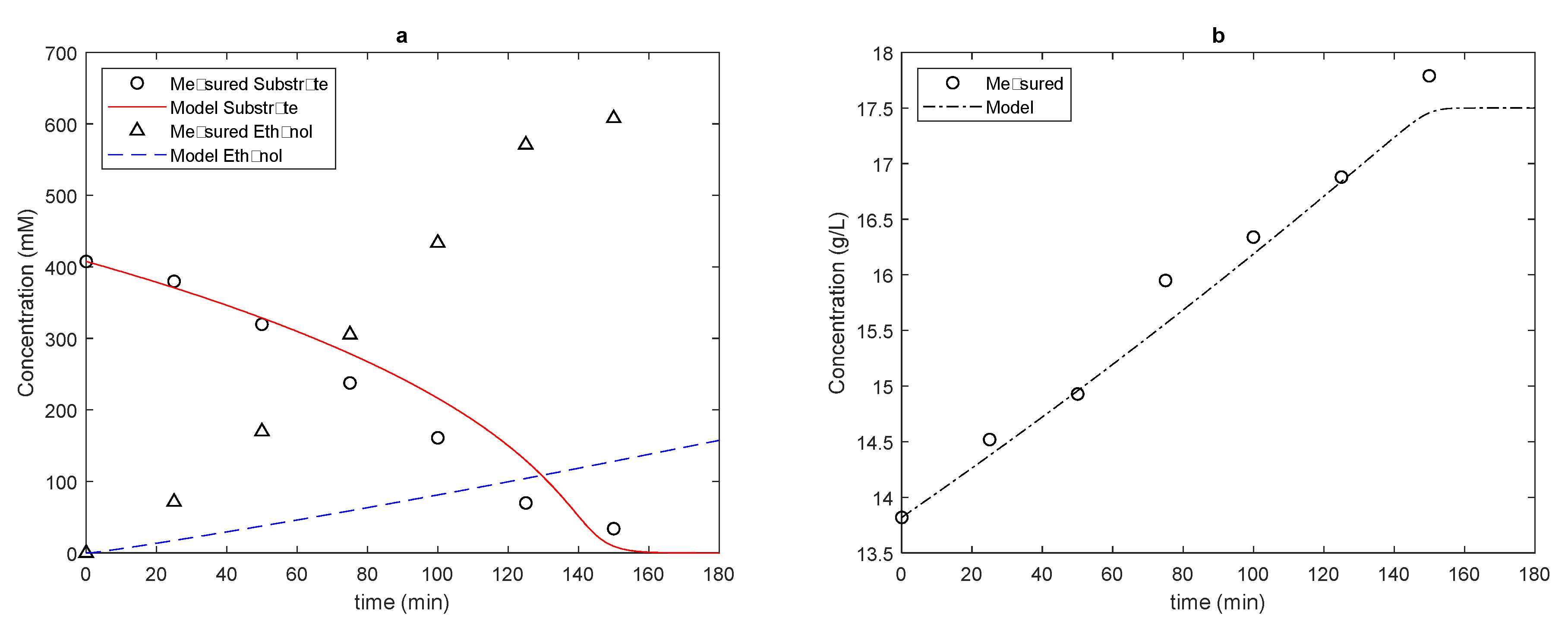
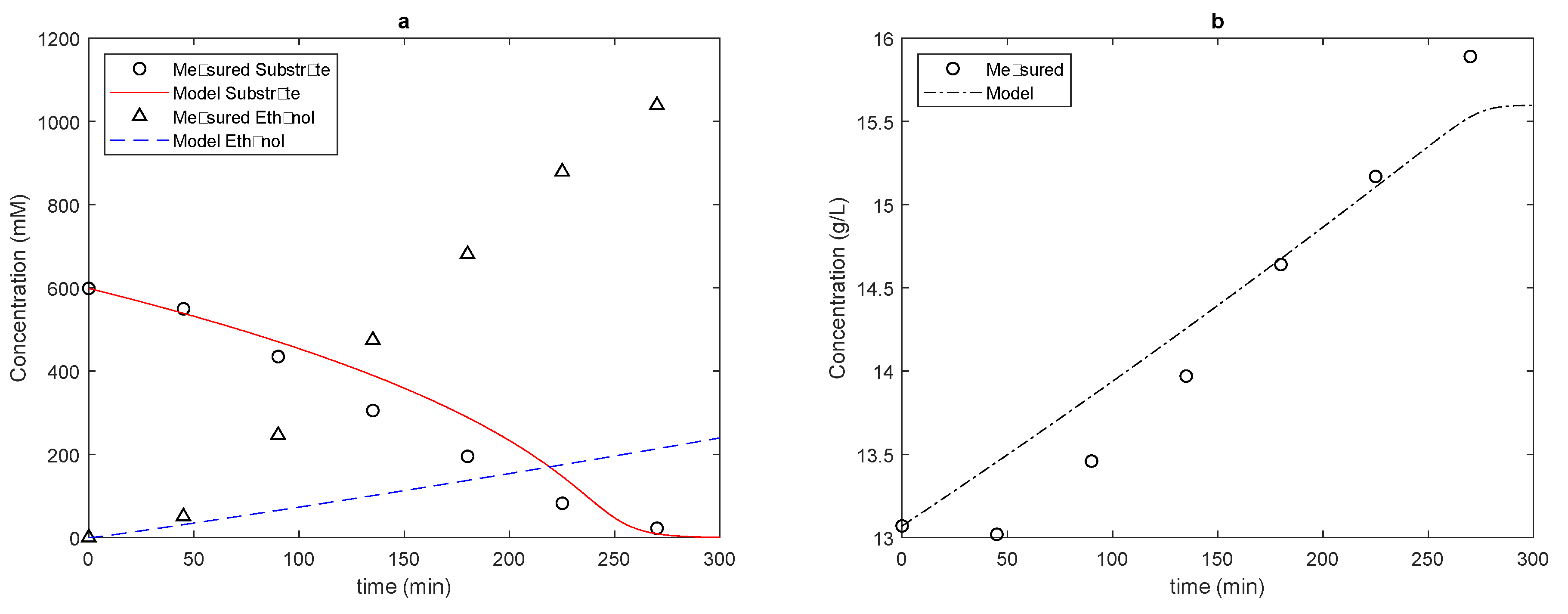
Figure 4, we present the results obtained by the SR model with the conditions described above.
In the three cases analyzed, we obtained a good fit for both the cell concentration and substrate consumption. However, for product formation, the results found were very poor: in none of the cases was product formation minimally close to the experimental values.
When we added the ramifications to the model, that is, when we run the model with branches, we obtained the results shown in Figure 5, Figure 6 and Figure 7.
Note that the prediction of product formation improves considerably with the addition of branches, even using extremely simple expressions such as those assumed in the present work. Thus, there is an indication that the addition of well-described ramifications to the metabolic model can further improve the results.
Considering the difference obtained between the models, we can compare the kinetic constants that most interfere in the response of the models, starting with the kinetic constants of the limiting step of alcoholic fermentation, i.e., the transport of glucose from the extracellular medium to the intracellular medium. Starting with the saturation constant KGLC, we noticed that the increase in the concentration of the substrate in the medium decreased the microorganism’s affinity for glucose: in the analyzed fermentations, medium- to low-affinity transporters were found, with this constant varying from 6.95 to 54 mM. In both models, we found the highest affinity in the situation with the lowest substrate concentration, matching the need for yeast cells to facilitate substrate entry under nutrient-scarce conditions. Furthermore, we noted that the CR model needed slightly higher saturation constants, except in the fermentation with a higher initial substrate concentration. Furthermore, in the more concentrated fermentation, the saturation constant for the two cases with a greater availability of microorganisms in the CR model was repeated, something not seen in the SR model. This point may also indicate the need to investigate whether yeast can express different transport proteins at different stages of fermentation, according to the availability of the substrate in the medium: in the present work, the concentrations of relevant enzymes and proteins were constants, since including kinetic expressions for their expression in different phases of the fermentation process is a future step for the development of metabolic models.
As for the maximum substrate conversion speed, there was an increase in this parameter with increasing concentration, and in the case of the CR model, the maximum glucose transport speed was reached at a lower concentration of substrate available in the medium. Better results for substrate consumption can eventually be obtained by working without considering a very simple substrate composed only of glucose.

4. Conclusions

The present work aimed to propose a model for a batch alcoholic fermentation process using a series of kinetic equations derived from the metabolism of Saccharomyces cerevisiae. Considering the ease and efficiency of the fungus Saccharomyces cerevisiae in carrying out alcoholic fermentation, in addition to the fact that this fungus is a quasi-model organism, we successfully assembled a model capable of predicting sugar consumption and the formation of ethanol using the relevant metabolic network. This setup was certainly simple because the fungus considered in the present study is a quasi-model microorganism, and the central metabolic route, the EMP route, is well studied. The biggest difficulties arose with the ramifications of this route, which have not been sufficiently studied and lack information. However, even the simplified use of these ramifications showed an improvement in the results of the proposed models, especially for the formation of ethanol, which was closer to reality with the CR model. This work can still be improved by giving more detail to the kinetics of the relevant branches. Andrews and Noack’s model sufficiently represents cell growth, but it is a black box model; if we add the kinetic relationships from metabolism, its contribution would be improved. Thus, we have in our hands a basic metabolic model that shows promise for the representation and study of batch alcoholic fermentation, which can be improved and optimized in the future.

Author Contributions

Conceptualization, R.L.A. and M.Y.G.D.G.; methodology, R.L.A., J.E.O. and C.M.G.A.; software, R.L.A. and C.M.G.A.; validation, R.L.A.; formal analysis, R.L.A.; investigation, R.L.A. and M.Y.G.D.G.; resources, R.L.A. and M.Y.G.D.G.; data curation, R.L.A., J.E.O.; writing—original draft preparation, R.L.A. and M.Y.G.D.G. and C.M.G.A.; writing—review and editing, R.L.A. and M.Y.G.D.G.; visualization, R.L.A. and J.E.O.; supervision, J.E.O. and C.M.G.A.; project administration, R.L.A. and J.E.O.; funding acquisition, R.L.A. and M.Y.G.D.G. All authors have read and agreed to the published version of the manuscript.

Funding

This study was funded by the Coordenação de Aperfeiçoamento de Pessoal de Nível Superior-Brasil (CAPES)-Finance Code 001-and by Conselho Nacional de Desenvolvimento Científico e Tecnológico-CNPq (Grant Number 162382/2018-9). The APC was funded by This work was partially supported by Conselho Nacional de Desenvolvimento Científico e Tecnológico-CNPq (Grant Number 162382/2018-9).

Conflicts of Interest

The authors declare no conflict of interest.

List of Acronyms and Abbreviations

ACAAcetaldehyde
ACEAcetate
ADHAlcohol dehydrogenase
ADPAdenosine diphosphate
ALDAldolase
ARTTotal reducing sugars
ATPAdenosine triphosphate
BPG1,3-bisphosphoglycerate
DHAPDihydroxyacetone-phosphate
EMPEmbden–Meyerhof–Parnas Route
ENOEnolase
EtOHEthanol
exWhen used as a subscript, it indicates an extracellular substance
FKFructokinases
F16Pβ-D-fructose-1,6-bisphosphate
F26PFructose-2,6-bisphosphate
F6Pβ-D-fructose-6-phosphate
FRUFructose
G1Pα-D-Glucose-1-phosphate
G3PDHGlycerol-3-Phosphate Dehydrogenase
G6Pα-D-Glucose-6-phosphate
GAPGlyceraldehyde-3-phosphate
GAPDHGlyceraldehyde-3-phosphate dehydrogenase
GLCexα-D-Extracellular glucose
GLCinα-D-Intracellular glucose
GLYGlycerol
grKinetic parameter of the PFK enzyme
HKHexokinase
HXTLarge family of hexose transporters
inWhen used as a subscript, it indicates an intracellular substance
PDCPyruvate decarboxylase
P2G2-phosphoglycerate
P3G3-phosphoglycerate
PEPPhosphoenolpyruvate
PFPentose-phosphate route
PFKPhosphofructokinase
PGKPhosphoglycerate Kinase
PGMPhosphoglyceratomutase
PHIPhosphohexoisomerase
PYRPyruvate
PYKPyruvatokinase
SUCCSuccinate
T6PTrehalose-6-phosphate
TPITriose-phosphate-isomerase
TRETrehalose
TRIO or Trio-PTriose-phosphate
ΓRatio for the mass action

Appendix A. Kinetic Equations Used

Since it is expected that this process of GLC entry into the intracellular environment is similar to an enzymatic process, as it is a process of facilitated diffusion, Teusink et al. [17] presented the following symmetric carrier model for the speed of glucose transport to the intracellular medium, v H X T :
v H X T , G = V m H X T [ G L C e x ] [ G L C i n ] K M , G L C + [ G L C e x ] + [ G L C i n ] + K i c K M , G L C [ G L C e x ] [ G L C i n ]
For the reaction catalyzed by HK, van Eunen et al. [16] proposed a model with allosteric regulation and the action of trehalose-6-phosphate, T6P:
v H K = V m a x [ G L C i n ] [ A T P ] K M , H K G L C K M , H K A T P [ G 6 P ] [ A D P ] K M , H K G L C K M , H K A T P K e q , H K ( 1 + [ G L C i n ] K M , H K G L C + [ G 6 P ] K M , H K G 6 P + [ T 6 P ] K M , H K T 6 P ) ( 1 + [ A T P ] K M , H K A T P + [ A D P ] K M , H K A D P )
For the action of phosphohexoisomerase, a relatively simple equation was used, representing the reversible kinetic equation of a substrate and a product:
v P H I = V m a x [ G 6 P ] K M , P H I G 6 P [ F 6 P ] K M , P H I F 6 P K e q , P H I 1 + [ G 6 P ] K M , P H I G 6 P + [ F 6 P ] K M , P H I F 6 P
Phosphofructokinase is a widely studied enzyme and much of its structure is known, but mathematically modeling its action is something extremely complex. Such is the level of complexity of the kinetic modeling of this enzyme that Teusink et al. [17] refer to such a process as the modelers’ nightmare. This enzyme has a huge amount of regulatory interactions, which means that the model of this enzyme needs to be considerably simplified to become practicable: no known model available for this enzyme can describe all the effects and interactions. Among the simplifications used in modeling this route, Teusink et al. [17] and van Eunen et al. [16] highlighted the hypothesis that some substances present constant concentrations throughout the fermentation process: ammonia, phosphate, protons, and the substance fructose-2,6-bisphosphate.
Among the regulatory effects known to act on this enzyme, the following three stand out: the cooperative binding of fructose-6-phosphate for the proper functioning of the enzyme, the inhibitory effect of ATP, and activation linked to adenosine monophosphate, AMP. Another considerable effect observed in the behavior of PFK is the lack of inhibition caused by its product, fructose-1,6-bisphosphate. However, this product negatively interferes with the activation of the enzyme produced by fructose-2,6-bisphosphate [16,17].
We expect that the kinetic model of the action of this enzyme includes the concentrations of the substances F6P, F16P, F26P, AMP, and ATP. Assuming that the effects of AMP, F26P, and F16P and the inhibitory effect of ATP are mediated by a shift in the balance between a tense and a relaxed state, the kinetics of this enzyme will be affected by an equilibrium constant between these states, symbolized by L. As the tense state is the state where the enzyme is inactive because there is no binding to F6P, Teusink et al. [17] and van Eunen et al. [16] proposed the use of the following kinetic model:
v P F K = V m a x g R λ 1 λ 2 R R 2 + L T 2
Being that
λ 1 = [ F 6 P ] K M , P F K F 6 P
λ 2 = [ A T P ] K M , P F K A T P
R = 1 + λ 1 λ 2 + g R λ 1 λ 2
T = 1 + c A T P λ 2
L = L 0 ( 1 + C i , A T P α 1 1 + α 1 ) 2 ( 1 + C i , A M P α 2 1 + α 2 ) 2 ( 1 + C i , F 2 , 6 P α 3 + C i , F 1 , 6 P α 4 1 + α 3 + α 4 ) 2
α 1 = [ A T P ] K P F K , A T P
α 2 = [ A M P ] K P F K , A M P
α 3 = [ F 26 P ] K P F K , F 26 P
α 4 = [ F 16 P ] K P F K , F 16 P
Of the constants to be used in this model, we have g R = 5 , 12 and L0 = 0.66, according to Teusink et al. [17] and van Eunen et al. [16].
For the action of the ALD enzyme, it is generally assumed to be a “uni–bi”-ordered kinetics, and this mechanism is represented by the following equation:
v A L D = V m a x a K a ( 1 Γ K e q , A L D ) 1 + a K M , F 16 p + p K p + q K q + a q K a K i q + p q K p K q
In (A14), it represents the F16P concentration, the DHAP concentration, and the GAP concentration. Furthermore, Ki indicates the saturation constant of this enzyme for each of the substances involved, and Kiq indicates an inhibition constant. This equation expands in a particular way, which we show below, taking into account a different way of writing the GAP concentration [16,17,24].
There are not many studies of this enzyme from Saccharomyces cerevisiae contributing the kinetic data of the model presented in (A14). The parameter with the most values found in the literature is the saturation constant for F16P, which is around 0.30 mM [16,17,24].
For the glycerol branch, Teusink et al. [17] indicated that the flux is completely controlled by the action of the G3PDH enzyme. The mechanism of action of this enzyme is not very well known yet, and some modeling works use a model similar to the action of HK, that is, a reversible reaction model with two substrates and two products, shown by Equation (A2), DHAP and NADH being the substrates, and glycerol-3-phosphate, GLY, and NAD+ the products.
To close the glycolysis preparation step, DHAP must be converted into GAP. This reaction is also mediated by a single enzyme, TPI. The kinetics of this TPI enzyme present, according to Smallbone et al. [24], direct the inhibition of DHAP in a particular way:
v T P I = V m a x [ D H A P ] K M , T P I D H A P [ D H A P ] ( 1 + ( [ D H A P ] 4 ) 4 )
However, it is common for this reaction to be considered in equilibrium, so it is customary not to consider the action of this enzyme in the glycolytic model. For such a condition, the equilibrium constant is used:
K e q , T P I = [ G A P ] [ D H A P ]
Since the value of the constant is around 0.045, the total amount of triose-phosphate, TRIO, in the cell is defined as
[ T R I O ] = [ G A P ] + [ D H A P ]
As a mathematical model for the GAPDH enzyme, a relationship similar to that of the action of HK can be used. However, van Eunen et al. [16] suggested improving this relationship with the use of two distinct maximum speeds, one for the direct reaction, V m a x + , and one for the reverse reaction, V m a x :
v G A P D H = V m a x + [ G A P ] ( [ N A D ] [ N A D H ] ) K M , G A D P H G A P K M , G A D P H N A D V m a x [ B P G ] [ N A D H ] K M , G A D P H B P G K M , G A D P H N A D H ( 1 + [ G A P ] K M , G A D P H G A P + [ B P G ] K M , G A D P H B P G ) ( 1 + [ N A D ] K M , G A D P H N A D + [ N A D H ] K M , G A D P H N A D H )
The next enzyme, PGK, presents a complicated kinetic study, according to Teusink et al. [17], because the BPG substrate is very unstable. Thus, it is more common to have data from the reverse reaction catalyzed by PGK, which is where most of the kinetic data for this reaction are taken from. Thus, it is customary to use the kinetic model of the reversible reaction with two substrates and two products for this enzyme, the substrates being BPG and ADP, and the products P3G and ATP, as shown in Equation (A19):
v P G K = V m a x K e q , P G K [ B P G ] [ A D P ] K M , P G K B P G K M , P G K A D P [ P 3 G ] [ A T P ] K M , P G K 3 P G K M , P G K A T P ( 1 + [ B P G ] K M , P G K B P G + [ P 3 G ] K M , P G K 3 P G ) ( 1 + [ A D P ] K M , P G K A D P + [ A T P ] K M , P G K A T P )
In the next reaction, we have the action of PGM, an enzyme that is dependent on the concentration of 2,3-diphosphoglycerate. To circumvent this dependence, thus reducing the model’s variables, some authors simply assume that the enzyme is already saturated with this substance at concentrations at micromolar levels. Even with these considerations, there is considerable variability in the values of the saturation constants of this reaction for P3G. Therefore, such a reaction can be modeled using a simple reversible reaction mechanism, with one substrate and one product only, as shown in the reaction below:
v P G M = V m a x [ P 3 G ] K M , P G M P 3 G [ P 2 G ] K M , P G M P 3 G K e q , P G M 1 + [ P 2 G ] K M , P G M P 3 G + [ P 2 G ] K M , P G M P 2 G
The conversion of P2G to PEP is one of the last reactions of glycolysis, a reaction catalyzed, under conditions of low growth, by only one enzyme, enolase (ENO). Kinetically, the model used to assess the action of this enzyme is similar to that used in PGM modeling, that is, a reversible reaction model with a substrate and a product:
v E N O = V m a x [ P 2 G ] K M , E N O P 2 G [ P E P ] K M , E N O P E P K e q , E N O 1 + [ P 2 G ] K M , E N O P 2 G + [ P E P ] K M , E N O P E P
Finally, closing the glycolysis, the last reaction consists of the conversion of PEP to PYR by a reaction catalyzed by the PYK enzyme. A striking feature of this enzyme is the strong dependence on F16P for its activation: under conditions of high concentrations of F16P, it exhibits hyperbolic behavior and a good affinity with PEP. This condition of a high F16P concentration was determined to be around 0.5 mM F16P, which is 10 times lower than the common value of such a metabolite in a cell under normal fermentative conditions. Therefore, hyperbolic modeling may prove adequate for this enzyme, the reaction being reversible, with two substrates and two products, and with F16P presenting an allosteric regulation, as shown in the equation below, proposed by van Eunen et al. [16]:
v P Y K = V m a x [ P E P ] K M , P Y K P E P ( [ P E P ] K M , P Y K P E P + 1 ) n 1 L 0 , P Y K ( [ A T P ] K M , P Y K A T P + 1 [ F 16 P ] K M , P Y K F 16 P + 1 ) n + ( [ P E P ] K M , P Y K P E P + 1 ) n A D P A D P + K M , P Y K A D P
Now, the alcoholic fermentation begins. This step consists of only two reactions that will lead to pyruvate being converted to ethanol, and the first metabolite to appear in this phase is acetaldehyde, produced by a reaction catalyzed by the PDC enzyme. This enzyme has cooperative kinetics, linked to the concentration of PYR in the medium, being a relatively simple model:
v P D C = V m a x [ P Y R ] n P D C K M , P D C P Y R ( [ P Y R ] n P D C K M , P D C P Y R n P D C + 1 )
Finally, there is the last reaction of the metabolic network under study: the conversion of ACA into ETOH and carbon dioxide by the action of ADH enzymes, whose kinetic behavior is considerably complex, being a bi-ordered mechanism with binding by a cofactor first:
v A D H = V m a x α A D H 1 + β A D H + γ A D H + δ A D H + ε A D H
α A D H = ( [ N A D ] [ N A D H ] ) [ E t O H ] K i , A D H N A D K M , A D H E t O H [ N A D H ] [ A C A ] K i , A D H N A D K M , A D H E t O H K e q , A D H
β A D H = [ N A D ] [ N A D H ] K i , A D H N A D + K M , A D H N A D [ E t O H ] K i , A D H N A D K M , A D H E t O H + K M , A D H N A D H [ A C A ] K i , A D H N A D K M , A D H A C A
γ A D H = ( [ N A D ] [ N A D H ] ) [ E t O H ] K i , A D H N A D K M , A D H E t O H + K M , A D H N A D H ( [ N A D ] [ N A D H ] ) [ A C A ] K i , A D H N A D K i , A D H N A D H K M , A D H A C A
δ A D H = [ N A D H ] K i , A D H N A D H + K M , A D H N A D [ N A D H ] [ E t O H ] K i , A D H N A D K i , A D H N A D H K M , A D H E t O H + [ N A D H ] [ A C A ] K i , A D H N A D H K M , A D H A C A
ε A D H = ( [ N A D ] [ N A D H ] ) [ E t O H ] [ A C A ] K i , A D H N A D K M , A D H E t O H K i , A D H A C A + [ N A D H ] [ E t O H ] [ A C A ] K i , A D H E t O H K i , A D H N A D H K M , A D H A C A
ADH lacks data for inhibition constants in the literature, but there are several studies on the saturation constant for different substrates at a pH of around 9.0 and different temperatures, ranging from 10 to 30 °C.

Appendix B. Tables with Kinetic Parameters Used in the Model

Table A1. Apparent turnover numbers (nmol min−1   mg s 1 ) of the SR and CR models according to the initial fermentation concentration.
Protein30 (g L−1)75 (g L−1)100 (g L−1)
HXT128,929165,200167,980
HK377,554354,849370,000
PHI874,243877,000877,000
PFK208,993209,980210,000
ALD535,408535,170535,500
GAPDH+1,973,4592,084,5952,090,000
GAPDH912,296840,000840,000
PGK2,125,0002,090,0002,160,000
PGM748,124840,000854,609
ENO345,772384,832439,400
PYK646,674718,020755,000
PDC172,954172,062172,000
ADH143,204143,000143,000
Table A2. Apparent saturation constants K (mM), equilibrium constants, and other constants of the SR and CR models as a function of the substance i according to the initial concentration of fermentation in g L−1.
9i3075100
K M , H X T GLC15,55227355750
K i C , H X T GLC0.90810.90810.9081
K M , H K GLC0.020.0180.02
K M , H K ATP0.250.250.25
K M , H K G6P30.0030.0030.00
K M , H K ADP0.240.240.24
K M , H K T6P0.200.200.15
K e q , H K -380038003800
K M , P H I G6P1.001.011.00
K M , P H I F6P0.310.310.31
K e q , P H I -0.3140.3140.314
K M , P F K F6P0.100.100.10
K M , P F K ATP0.710.710.71
K P F K ATP0.650.650.65
K P F K AMP0.09950.09950.0995
K P F K F16P0.1110.1110.111
K P F K F26P6.82·10−46.82·10−46.82·10−4
c i , P F K ATP333
C i , P F K ATP100100100
C i , P F K AMP0.08450.08450.0845
C i , P F K F16P0.3970.3970.397
C i , P F K F26P0.01740.01740.0174
g R , P F K -5.125.125.12
L 0 , P F K -0.660.660.66
K M , A L D F16P0.0550.0550.055
K M , A L D GAP2.002.002.00
K M , A L D DHAP2.402.402.40
K i , A L D GAP101010
K e q , A L D -0.0690.0690.069
K M , G A P D H GAP0.210.210.21
K M , G A P D H NAD0.090.090.09
K M , G A P D H BPG1.181.181.18
K M , G A P D H NADH0.10.10.1
K M , P G K BPG3.00·10−33.00·10−33.00·10−3
K M , P G K ADP0.490.490.49
K M , P G K 3PG0.530.530.53
K M , P G K ATP0.300.300.30
K e q , P G K -320032003200
K M , P G M P3G1.081.091.10
K M , P G M P2G0.100.100.10
K e q , P G M -0.190.190.19
K M , E N O P2G0.0500.0500.050
K M , E N O PEP0.500.500.50
K e q , E N O -6.76.76.7
K M , P Y K PEP0.0210.0210.021
K M , P Y K ADP0.160.160.20
K M , P Y K F16P0.20.20.2
K M , P Y K ATP1.51.51.5
n P Y K -444
L 0 , P Y K -60,00060,00060,000
K M , P D C PYR850078288500
n P D C -1.91.91.9
K M , A D H NAD0.0590.0590.059
K M , A D H NADH0.1200.1100.122
K M , A D H ACA2.832.832.83
K M , A D H EtOH121212
K i , A D H NAD0.920.920.92
K i , A D H NADH0.0310.0310.031
K i , A D H ACA1.11.11.1
K i , A D H EtOH909090
K e q , A D H -6.9·10−56.9·10−56.9·10−5
K T R E , 1 -0.0830.4570.485
K T R E , 2 -00.2100.430
K G L Y -0.580.4990.121
K S U C -0.0300.0000.000
K A C E -0.1300.1520.000
Table A3. Apparent substrate transport turnover numbers (nmol min−1    mg s 1 ) of the SR and CR models according to the initial fermentation concentration.
Model30 (g L−1)75 (g L−1)100 (g L−1)
SR149.96216.00310,000
CR150.99310,000310,000
Table A4. Apparent substrate transport saturation constants KGLC (mM), equilibrium constants, and other constants of the SR and CR models as a function of the substance according to the initial concentration of fermentation in g L−1.
KiModel3075100
KiG,HXTGLCSR6.9517.554.0
CR8.4035.535.0

References

  1. Andrietta, M.G.S.; Andrietta, S.R.; Steckelberg, C.; Stupiello, E.N.A. Bioethanol—30 years of Proálcool. Int. Sugar J. 2007, 109, 195–200. [Google Scholar]
  2. Ferreira, R.J.A. Tecnologia de Produção de Alcool: Fermentação Alcoólica; Rio de Janeiro, Brazil, 2008; p. 73. [Google Scholar]
  3. Dai, Z.; Nielsen, J. Advancing metabolic engineering through systems biology of industrial microorganisms. Curr. Opin. Biotechnol. 2015, 36, 8–15. [Google Scholar] [CrossRef]
  4. Jonker, J.; van der Hilst, F.; Junginger, H.; Cavalett, O.; Chagas, M.; Faaij, A. Outlook for ethanol production costs in Brazil up to 2030, for different biomass crops and industrial technologies. Appl. Energy 2015, 147, 593–610. [Google Scholar] [CrossRef]
  5. Gaden, E.L., Jr. Fermentation process kinetics. J. Biochem. Microbiol. Technol. Eng. 1859, 1, 413–429. [Google Scholar] [CrossRef] [Green Version]
  6. Sonnleitner, B.; Käppeli, O. Growth of Saccharomyces cerevisiae is controlled by its limited respiratory capacity: Formulation and verification of a hypothesis. Biotechnol. Bioeng. 1986, 28, 927–937. [Google Scholar] [CrossRef]
  7. Birol, G.; Doruker, P.; Kirdar, B.; İlsen Önsan, Z.; Ülgen, K. Mathematical description of ethanol fermentation by immobilized Saccharomyces cerevisiae. Process. Biochem. 1998, 33, 763–771. [Google Scholar] [CrossRef]
  8. Kostov, G.; Popova, S.; Gochev, V.; Koprinkova-Hristova, P.; Angelov, M.; Georgieva, A. Modeling of Batch Alcohol Fermentation with Free and Immobilized Yeasts Saccharomyces cerevisiae 46 EVD. Biotechnol. Biotechnol. Equip. 2012, 26, 3021–3030. [Google Scholar] [CrossRef] [Green Version]
  9. Sainz, J.; Pizarro, F.; Pérez-Correa, J.R.; Agosin, E. Modeling of yeast metabolism and process dynamics in batch fermentation. Biotechnol. Bioeng. 2003, 81, 818–828. [Google Scholar] [CrossRef] [PubMed]
  10. De Freitas, H.F.S.; Olivo, J.E.; Andrade, C.M.G. Optimization of Bioethanol In Silico Production Process in a Fed-Batch Bioreactor Using Non-Linear Model Predictive Control and Evolutionary Computation Techniques. Energies 2017, 10, 1763. [Google Scholar] [CrossRef] [Green Version]
  11. Nielsen, J. Systems biology of metabolism. Annu. Rev. Biochem. 2017, 86, 245–275. [Google Scholar] [CrossRef]
  12. Takagi, Y.A.; Nguyen, D.H.; Wexler, T.B.; Goldman, A.D. The Coevolution of Cellularity and Metabolism Following the Origin of Life. J. Mol. Evol. 2020, 88, 598–617. [Google Scholar] [CrossRef]
  13. Keller, M.A.; Turchyn, A.V.; Ralser, M. Non-enzymatic glycolysis, and pentosentation phosphate pathway-like reactions in a plausible Archean ocean. Mol. Syst. Biol. 2014, 10, 12. [Google Scholar] [CrossRef] [PubMed]
  14. Nilsson, A.; Nielsen, J.; Palsson, B.O. Metabolic models of protein allocation call for the kinome. Cell Syst. 2017, 5, 4. [Google Scholar]
  15. Davidi, D.; Milo, R. Lessons on enzyme kinetics from quantitative proteomics. Curr. Opin. Biotechnol. 2017, 46, 81–89. [Google Scholar] [CrossRef]
  16. van Eunen, K.; Bakker, B.M. The importance and challenges of in vivo-like enzyme kinetics. Perspect. Sci. 2014, 1, 126–130. [Google Scholar] [CrossRef] [Green Version]
  17. Teusink, B.; Passarge, J.; Reijenga, C.A.; Esgalhado, M.; van der Weijden, C.C.; Schepper, M.; Walsh, M.C.; Bakker, B.M.; Van Dam, K.; Westerhoff, H.V.; et al. Can yeast glycolysis be understood in terms of in vitro kinetics of the constituent enzymes? Testing biochemistry. JBIC J. Biol. Inorg. Chem. 2000, 267, 5313–5329. [Google Scholar] [CrossRef]
  18. Sato, K.; Yoshida, Y.; Hirahara, T.; Ohba, T. On-line measurement of intracellular ATP of Saccharomyces cerevisiae and pyruvate during sake mashing. J. Biosci. Bioeng. 2000, 90, 294–301. [Google Scholar] [CrossRef]
  19. Ruoff, P.; Christensen, M.K.; Wolf, J.; Heinrich, R. Temperature dependency and temperature compensation in a model of yeast glycolytic oscillations. Biophys. Chem. 2003, 106, 179–192. [Google Scholar] [CrossRef]
  20. Casei, E.; Mosier, N.S.; Adamec, J.; Stockdale, Z.; Ho, N.; Sedlak, M. Effect of salts on the Co-fermentation of glucose and xylose by a genetically engineered strain of Saccharomyces cerevisiae. Biotechnol. Biofuels 2013, 6, 10. [Google Scholar] [CrossRef] [Green Version]
  21. Peeters, K.; Van Leemputte, F.; Fischer, B.; Bonini, B.M.; Quezada, H.; Tsytlonok, M.; Haesen, D.; Vanthienen, W.; Bernardes, N.; Gonzalez-Blas, C.B.; et al. Fructose-1,6-bisphosphate couples glycolytic flux to activation of Ras. Nat. Commun. 2017, 8, 922. [Google Scholar] [CrossRef] [PubMed]
  22. Teusink, B.; Diderich, J.A.; Westerhoff, H.V.; van Dam, K.; Walsch, M.C. Intracellular glucose concentration in derepressed yeast cells consuming glucose is high enough to reduce the glucose transport rate by 50%. J. Bacteriol. 1998, 180, 556–562. [Google Scholar] [CrossRef] [PubMed] [Green Version]
  23. Berthels, N.J.; Otero, R.R.C.; Bauer, F.F.; Pretorius, I.S.; Thevelein, J.M. Correlation between glucose/fructose discrepancy and hexokinase kinetic properties in different Saccharomyces cerevisiae wine yeast strains. Appl. Microbiol. Biotechnol. 2008, 77, 1083–1091. [Google Scholar] [CrossRef] [PubMed]
  24. Smallbone, K.; Messiha, H.L.; Carroll, K.M.; Winder, C.L.; Malys, N.; Dunn, W.B.; Murabito, E.; Swainston, N.; Dada, J.O.; Khan, F.; et al. A model of yeast glycolysis based on a consistent kinetic cha of all its enzymes. FEBS Lett. 2013, 587, 2832–2841. [Google Scholar] [CrossRef] [PubMed]
  25. Acorsi, R.L.; Moraes, F.F.; Olivo, J.E. Estudo da Fermentação Alcoólica Descontínua de Mel Invertido; VII EPCC: Maringá, Brasil, 2013. [Google Scholar]
  26. Sumner, J.B. Dinitrosalicylic acid reagent for the estimation of sugar in normal and diabetic urine. J. Biol. Chem. 1959, 47, 5–9. [Google Scholar] [CrossRef]
  27. Dove, G.B., III; Wilke, C.R.; Blanch, H.W. Process Development Studies for the Enhanced Recovery of Cellulase in Cellulose Hydrolysis. Master’s Thesis, Lawrence Berkeley Laboratory, University of California, Berkeley, CA, USA, 1981. [Google Scholar]
  28. Zanin, G.M.; Moraes, F.F. Tecnologia de Imobilização de Células e Enzimas Aplicada à Produção de Álcool de Biomassas. Relatório 1987, 2, 315–321. [Google Scholar]
Figure 1. Stoichiometric representation of the selected metabolic route consisting of the EMP route followed by alcoholic fermentation. Source: prepared by the authors.
Fermentation 08 00082 g001
Figure 2. (a) SR model result with an initial concentration of 30 g/L, and (b) adjustment of cell concentration. Source: prepared by the author.
Fermentation 08 00082 g002
Figure 3. (a) SR model result with an initial concentration of 75 g/L, and (b) adjustment of cell concentration. Source: prepared by the author.
Fermentation 08 00082 g003
Figure 4. (a) SR model result with an initial concentration of 100 g/L, and (b) adjustment of cell concentration. Source: prepared by the author.
Fermentation 08 00082 g004
Figure 5. (a) Result of the CR model with an initial concentration of 30 g/L, and (b) adjustment of cell concentration. Source: prepared by the author.
Fermentation 08 00082 g005
Figure 6. (a) Result of the CR model with an initial concentration of 75 g/L, and (b) adjustment of cell concentration. Source: prepared by the author.
Fermentation 08 00082 g006
Figure 7. (a) Result of the CR model with an initial concentration of 100 g/L, and (b) adjustment of cell concentration. Source: prepared by the author.
Fermentation 08 00082 g007
Table 1. Substances with constant concentrations in the model application. Source: van Eunen et al. [16].
SubstanceConcentration (mM)SubstanceConcentration (mM)
A T P 3 T 6 P 0.2
A D P 1 F 26 P 0.014
A M P 0.3 N A D 1.59
Table 2. Initial concentrations of the substrate, [ i ] 0 , product, and internal metabolites from alcoholic fermentation. Source: van Eunen et al. [16]; Sato et al. [18]; Teusink et al. [17]; Ruoff et al. [19]; Casei et al. [20]; Peeters et al. [21].
Substance (mM)[i]0 (mM)Substance (mM)[i]0 (mM)
GLCex*P3G1.09
GLCin0.1213P23G0.15
G6P0.50PEP0.11
F6P0.20PYR0.25
F16P1.80ACA0.04
TRIO0.50EtOH0.00
BPG0.05NADH0.29
* The initial value to be chosen.
Publisher’s Note: MDPI stays neutral with regard to jurisdictional claims in published maps and institutional affiliations.

