
Continuous Eddy Simulation vs. Resolution-Imposing Simulation Methods for Turbulent Flows

Abstract
:1. Introduction
- In this case, the hybrid RANS-LES model cannot properly handle the transition between RANS and LES regimes, which requires the model to increase (decrease) its contribution in response to a relatively low (high) actual flow resolution. Given the uncertainty of the actual flow resolution, there is implied uncertainty of simulation results. Hence, often unavailable validation data are required, and reliable predictions of very high- turbulent flows are out of reach.
- The mismatch between the imposed and actual flow resolution introduces hybridization errors (see the discussion of minimal error methods below). To accomplish a desired simulation performance, finer grids (higher computational cost) are then needed to minimize hybridization errors [17].
- The imbalance between the damping of fluctuations (controlled by the modeled viscosity) and the resolved fluctuations can generate problems seen very often in hybrid RANS-LES, which require the stimulation of fluctuations to trigger the development of instantaneous turbulence or the damping of fluctuations to prevent the shifting from RANS to LES within the boundary layer.
- What are characteristic general differences between CES methods and simulation methods that impose flow resolution independent of the actual resolved motion?
- Do the conceptual advantages of CES methods imply specific practical advantages, e.g., in regard to reliability of simulation results and computational cost?
- Which insight can be obtained from the application of CES methods to extreme regimes that cannot be reliably studied by any other approach?
2. Modeling and Computational Approach
2.1. CES Models Considered
2.2. Computational Approach
- The remaining flow terms were discretized using the second-order limitedLinearV scheme. The pressure–velocity coupling was handled by the PISO algorithm, which dynamically adjusts the pressure gradient along the flow direction to maintain a constant mass flow rate [30]. The iterative solution process employed a preconditioned bi-conjugate gradient technique with diagonally incomplete LU preconditioning for all flow variables except pressure at each time step [31]. To solve the Poisson equation for pressure, an algebraic multi-grid solver was utilized.
3. Hump Flow Simulation Set-Up
3.1. Flow Configuration
3.2. Boundary Conditions
- Hence, the predicted velocity and turbulence characteristics (turbulence kinetic energy) were systematically recorded in samples at the mapping plane during each iteration over time units. This compiled a comprehensive flow library. Samples were then extracted, extrapolated, and fed in as inflow conditions at the main simulation’s inlet plane. Figure 2 (right) shows the time-averaged streamwise velocity profile at the inlet plane (mapping plane). This profile closely resembles the velocity profile reported by You et al. [35] at the same axial position.
3.3. Simulation Set-Up
4. CES Model Performance
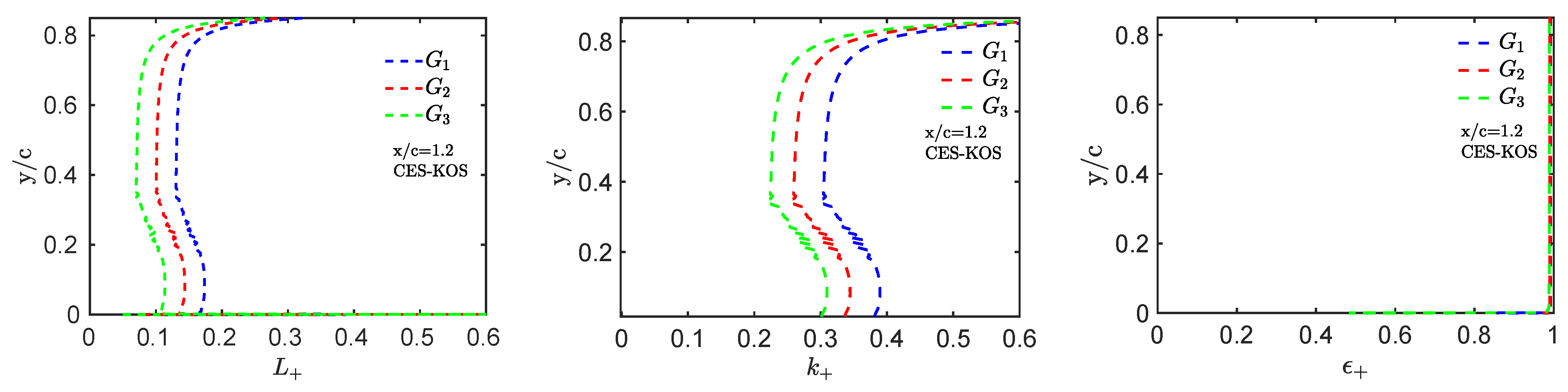
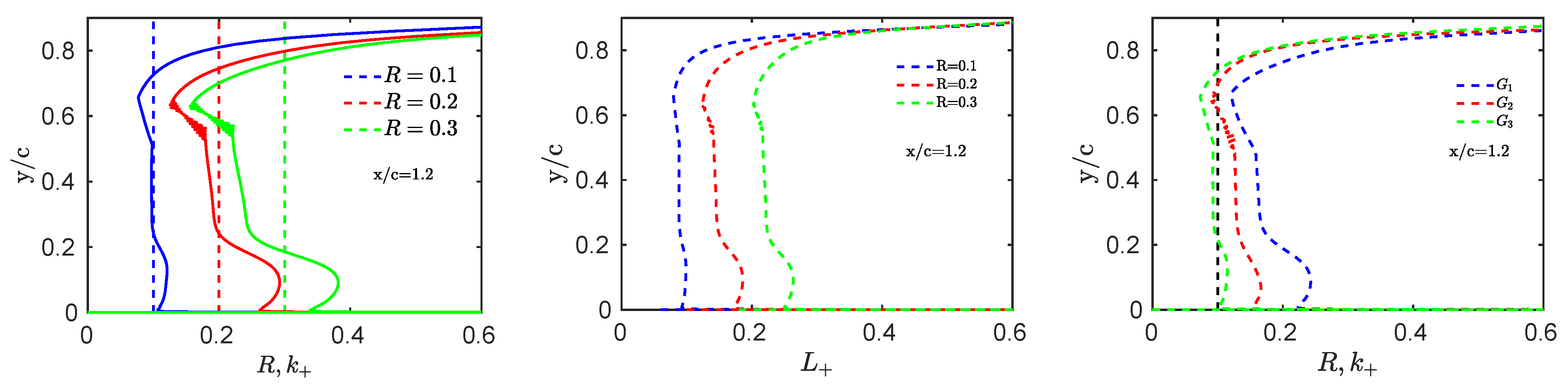
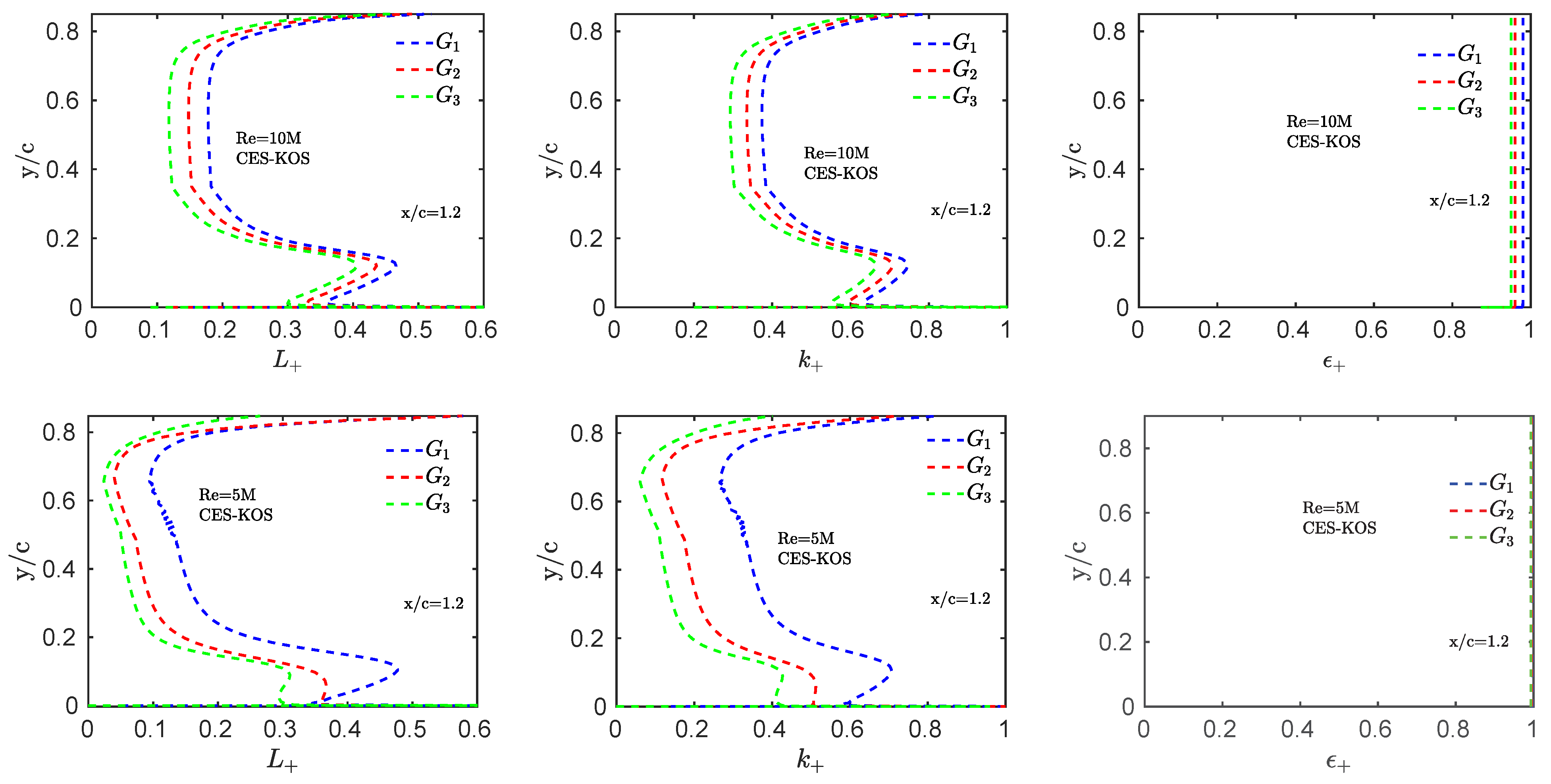
4.1. Resolution Variations
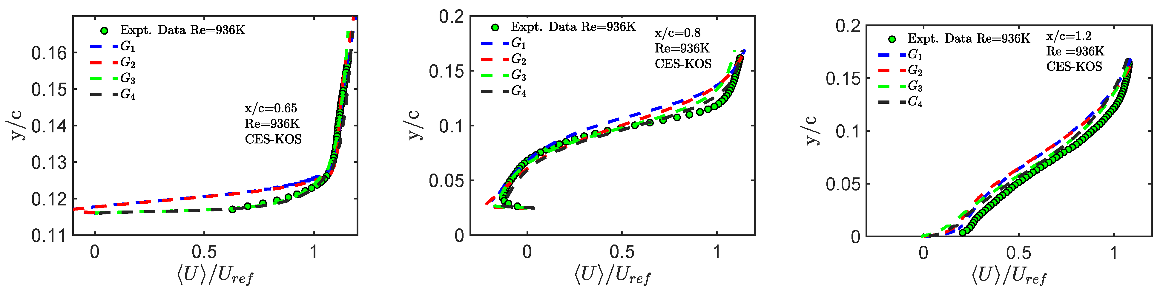
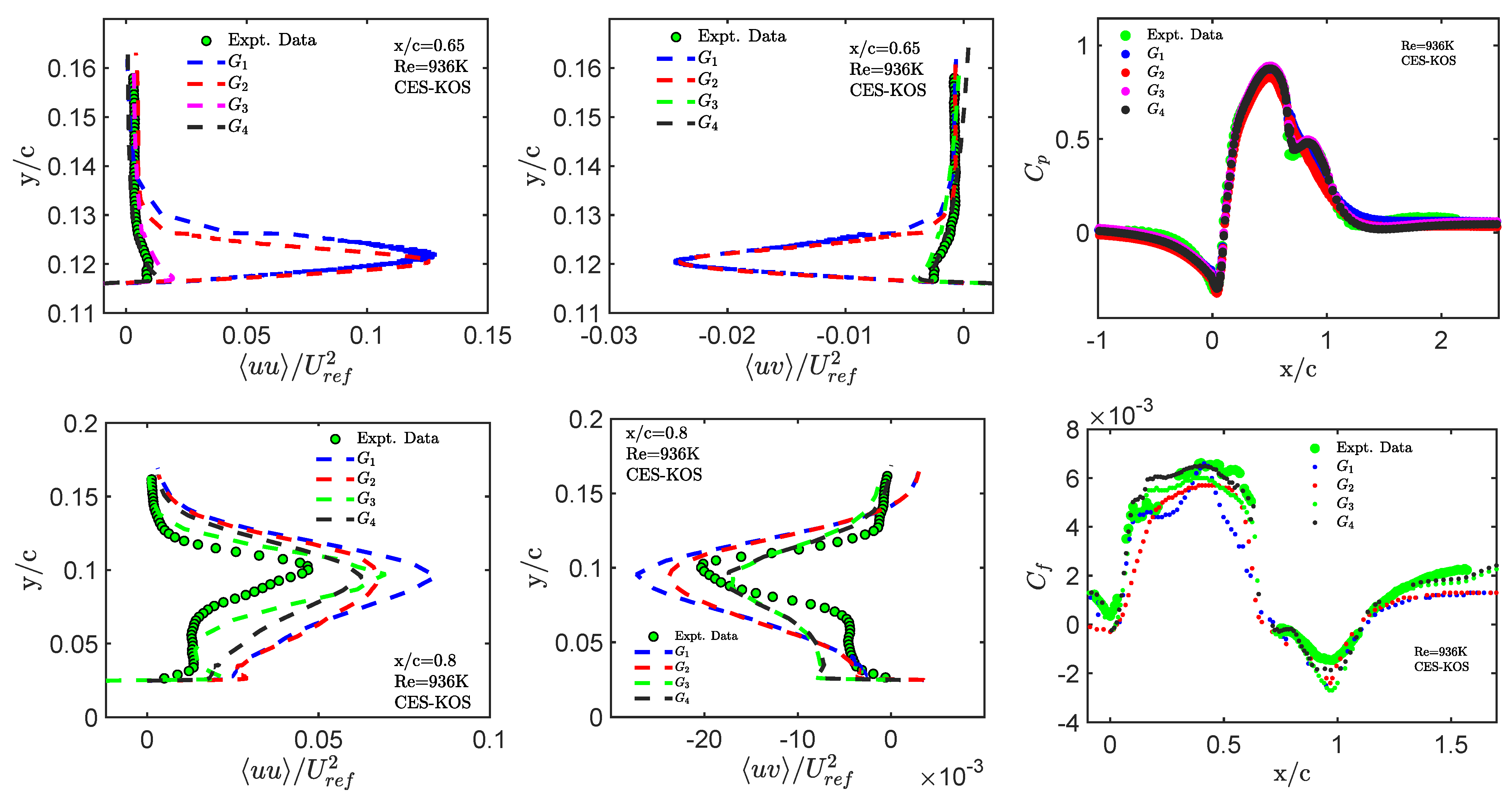
4.2. Flow Simulations
5. CES vs. Resolution Imposing Methods
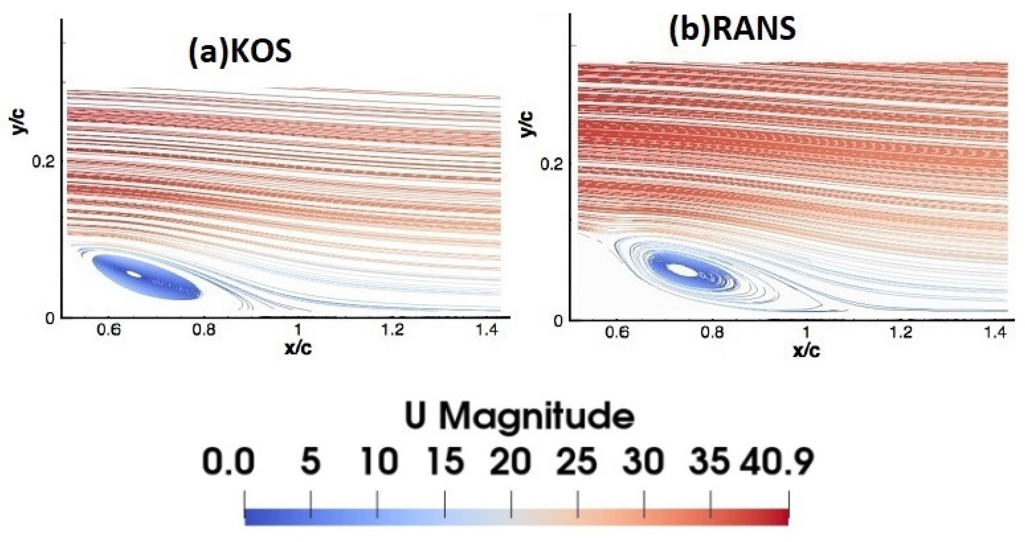
5.1. CES vs. RANS
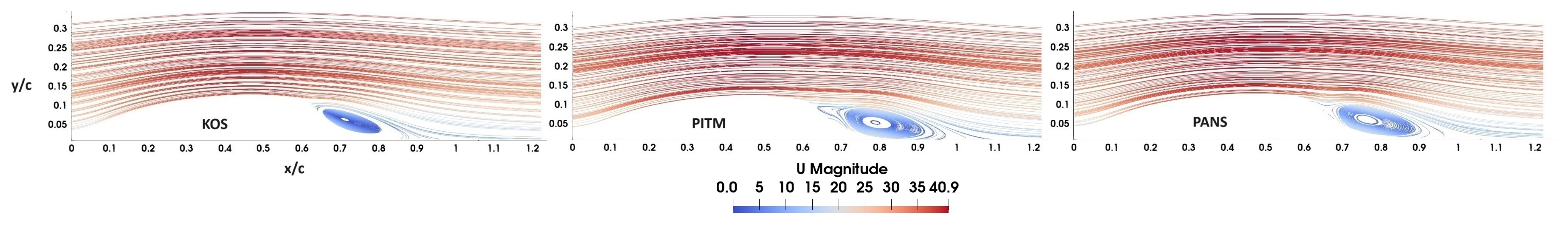
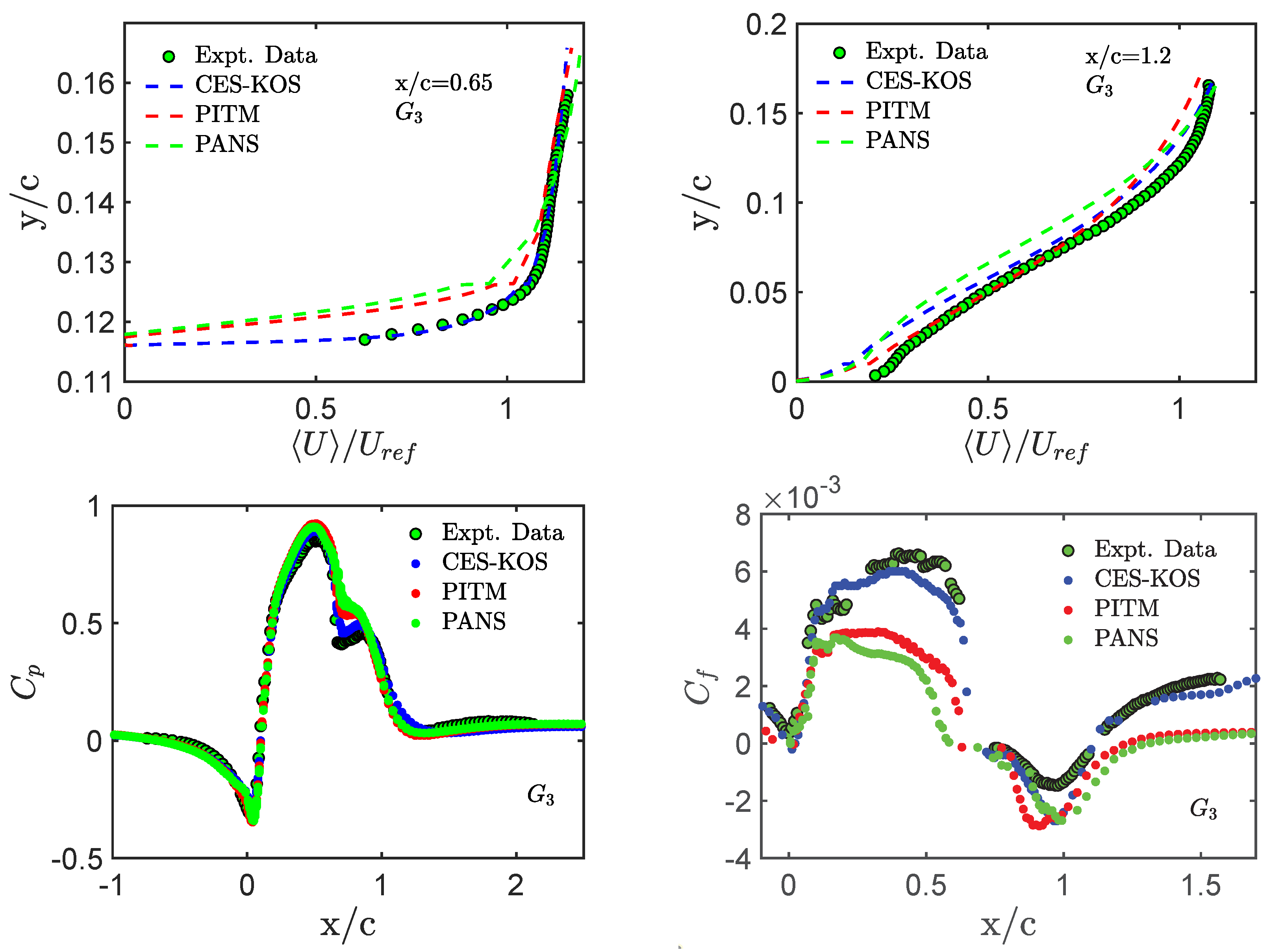
5.2. CES vs. PANS and PITM
5.3. CES vs. DES
6. CES vs. LES Methods
6.1. CES vs. LES
6.2. CES vs. WMLES, WRLES
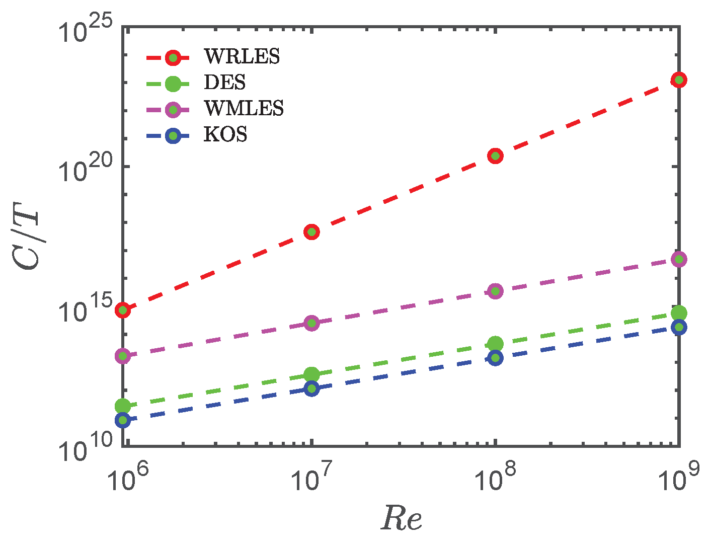
6.3. Cost Scalings
7. Very High-Re Simulations
7.1. Effects on Flow Resolution
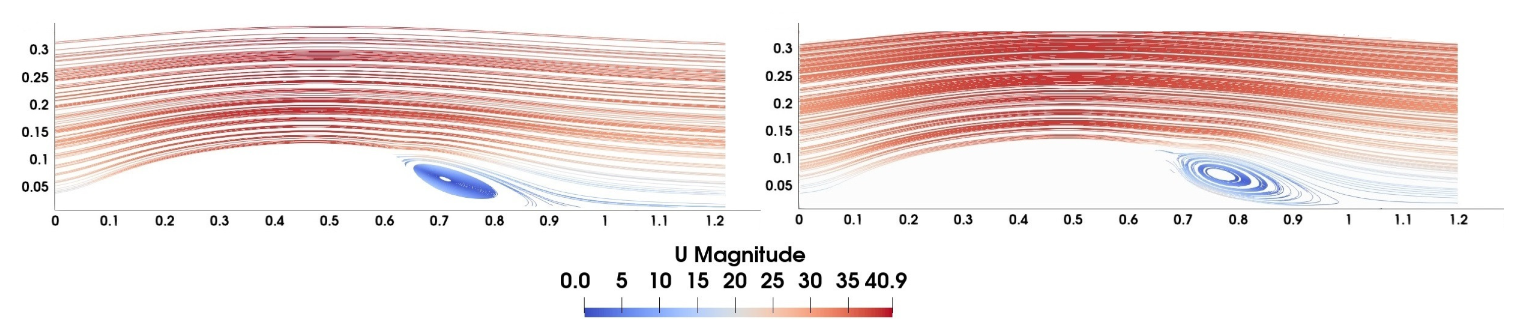
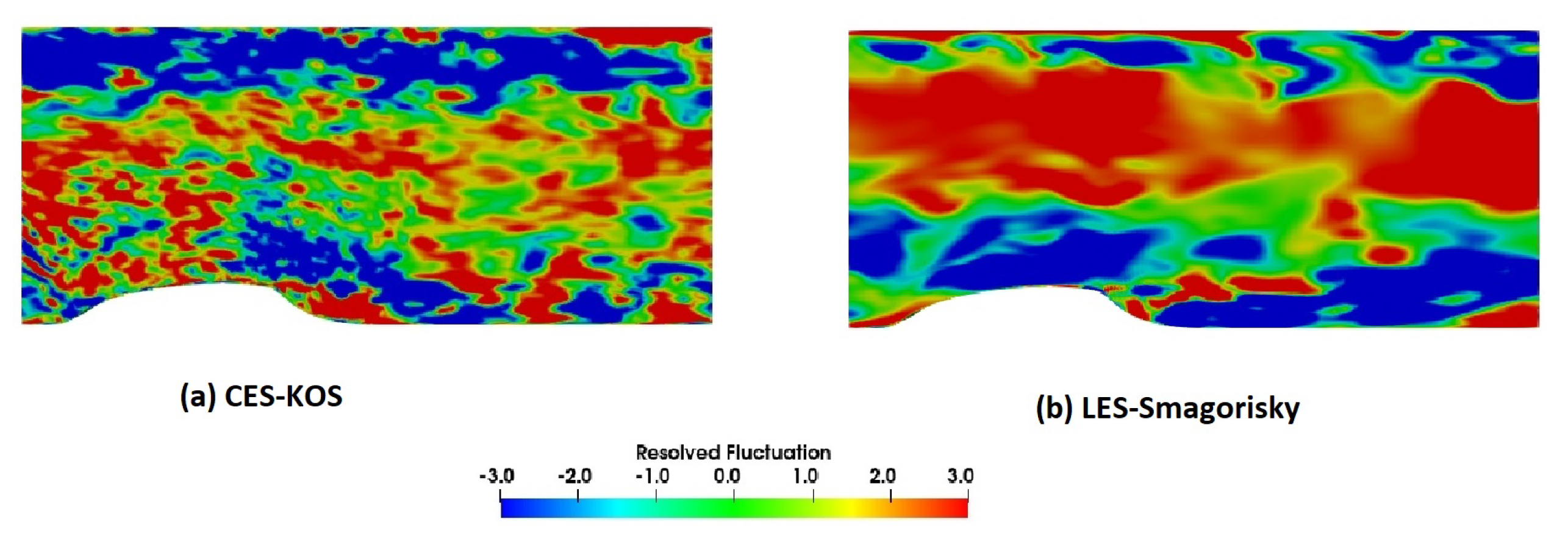
7.2. Effects on Flow Structures
7.3. Asymptotic Regime
8. Conclusions
- From a general viewpoint, the advantage of CES methods demonstrated here was an excellent simulation performance independent from adjustments of simulation settings. The latter advantage is based on the model’s ability to adjust the model to changing flow conditions (the amount of resolved motion). A grid dependence of simulation results was found if extremely coarse grids are applied.
- The implementation of a sensibilization of the model to the degree of flow resolution is not the only requirement to enable a performance as demonstrated here in regard to CES methods. An equally important condition is the mathematically correct implementation of an appropriate model sensitivity. The latter was demonstrated here via comparisons with PANS and PITM methods, demonstrating a simulation performance that is outperformed by CES methods.
- Contrary to CES, other popular simulation methods impose a certain desired flow resolution: this applies to RANS, LES, and other hybrid RANS-LES. This inherent model inflexibility generates a sensitive dependence on simulation parameter settings, for which optimal solutions cannot be found for every flow. In addition, this concept does not ensure that the desired imposed resolution is actually realized. This can imply higher computational cost (finer grids) to compensate for performance deficiencies [17].
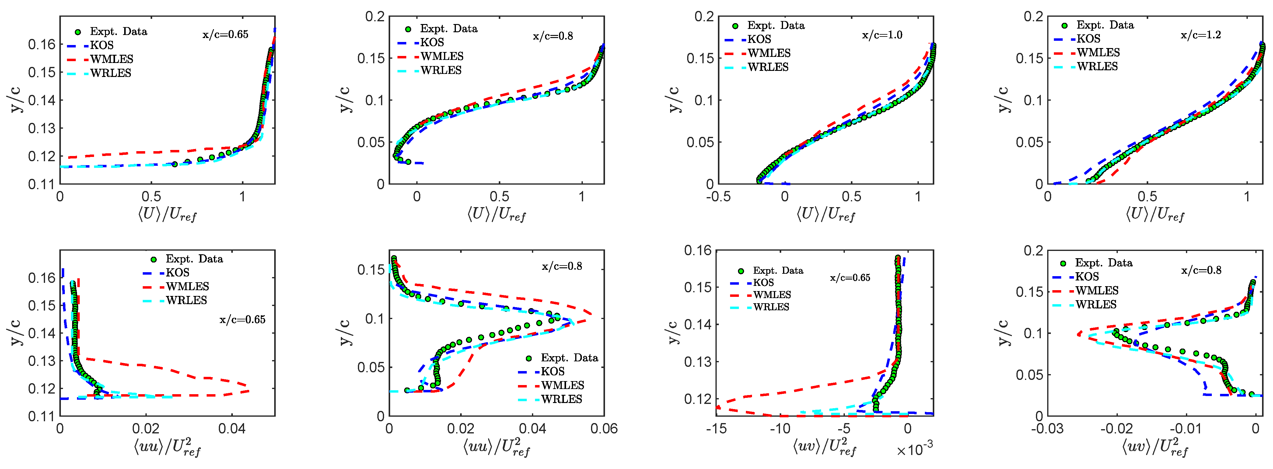
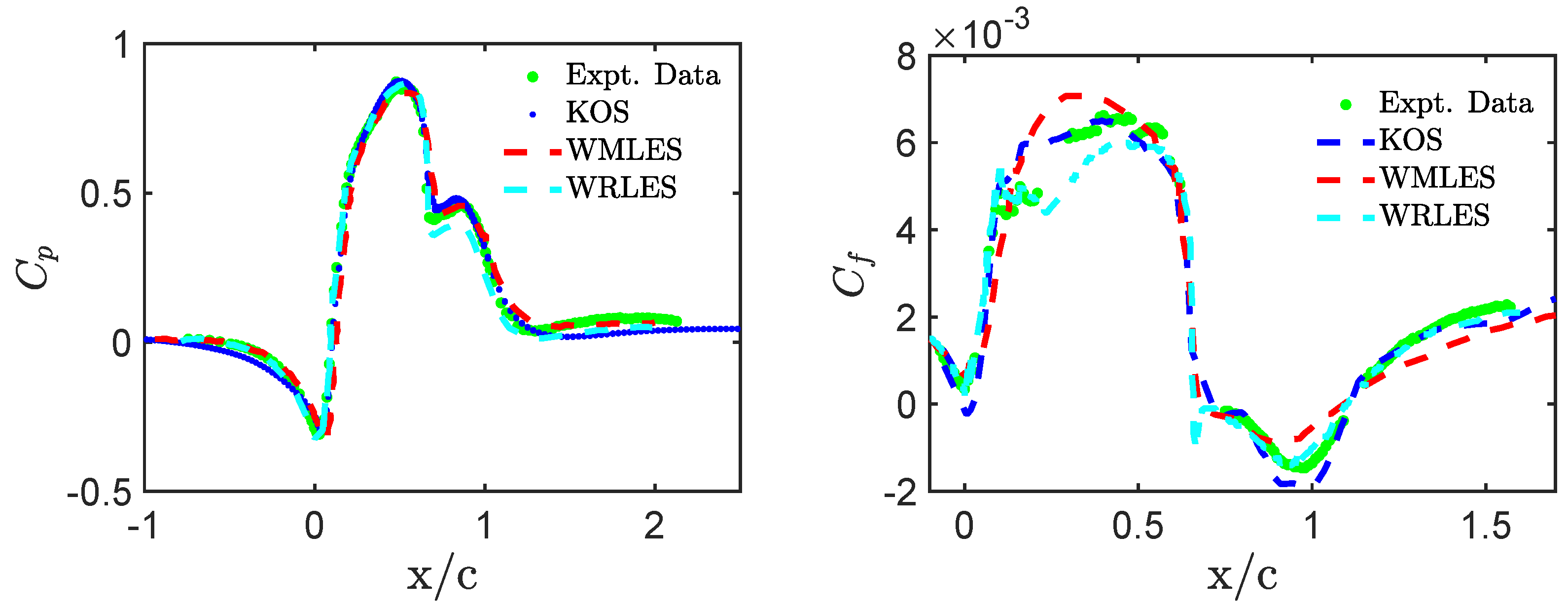
- Table 7 speaks a clear language in regard to the use of WRLES: for decades to come, WRLES will be inapplicable to many relevant turbulent flows. The use of WRLES also faces questions from a simulation performance view point. Figure 21, for example, shows that the use of WRLES is no guarantee for excellent simulation results. The latter can be attributed to a significant conceptual issue of WRLES: the inclusion of the filter width as length scale, which can be unphysical.
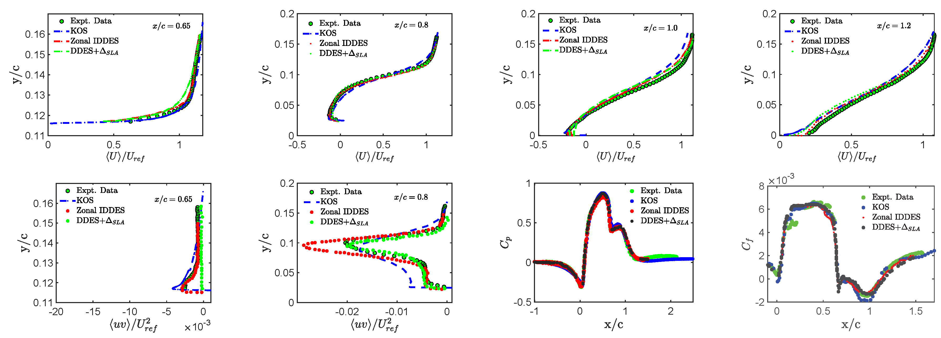
- The most popular hybrid RANS-LESes are DES and WMLES. Both depend on a variety of simulation settings, as specified here, which need to be adjusted to (often unavailable) validation data. The computational costs of DES and WMLES are well above the CES cost; see the discussion related to Table 7. Performance-wise, CES-KOS was shown to perform better than DES versions and WMLES. These differences may be attributed to the CES feature to be a minimal error simulation method.
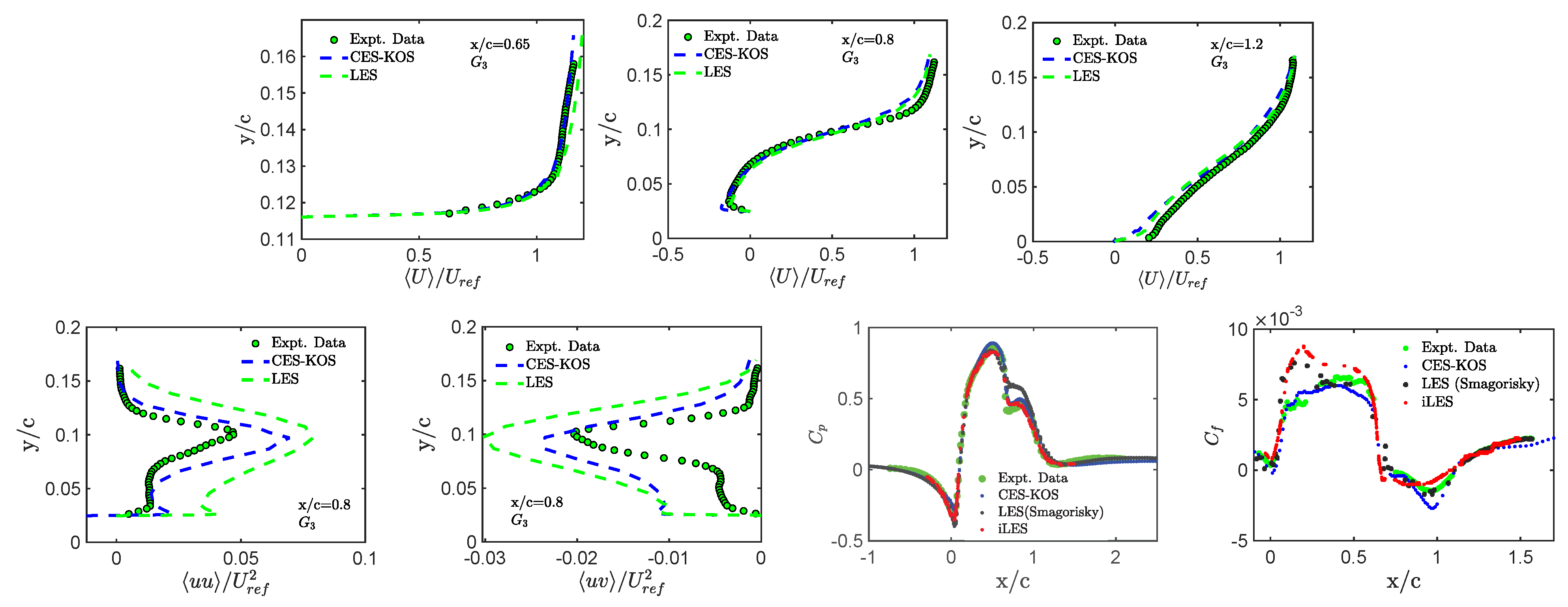
- PANS and PITM were introduced as alternatives to DES and WMLES. Figure 15 in conjunction with other related figures shows something interesting: the use of hybrid RANS-LES is no guarantee to obtain simulation results better than corresponding RANS prediction; the opposite may be the case. The underlying conceptual issue is the idea to impose a desired flow resolution. The latter does not only not determine the actual flow resolution, but the mismatch implied can deteriorate simulation results.
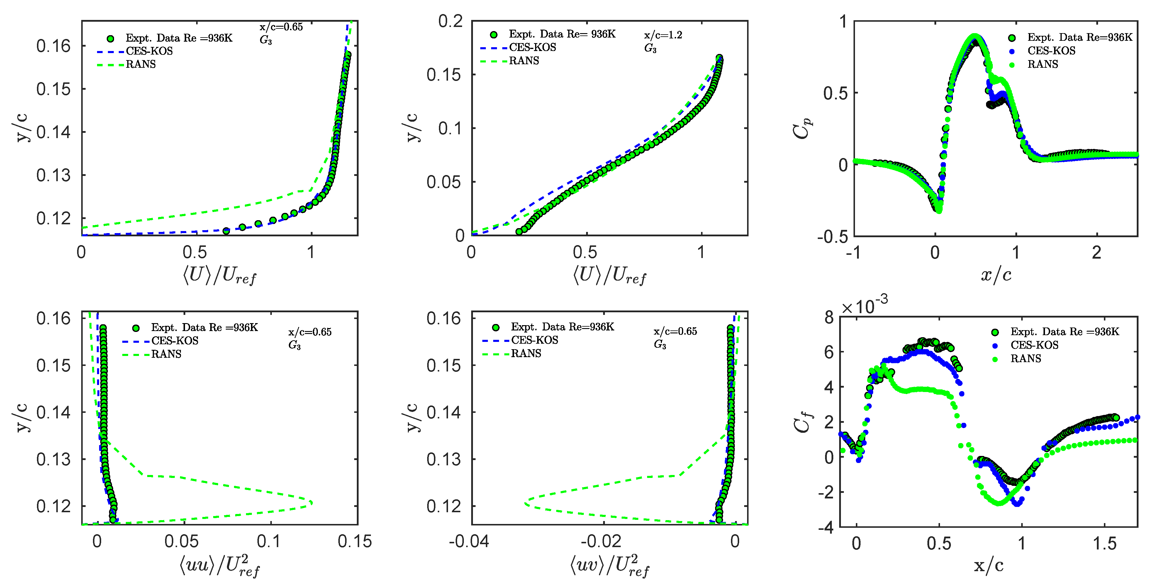
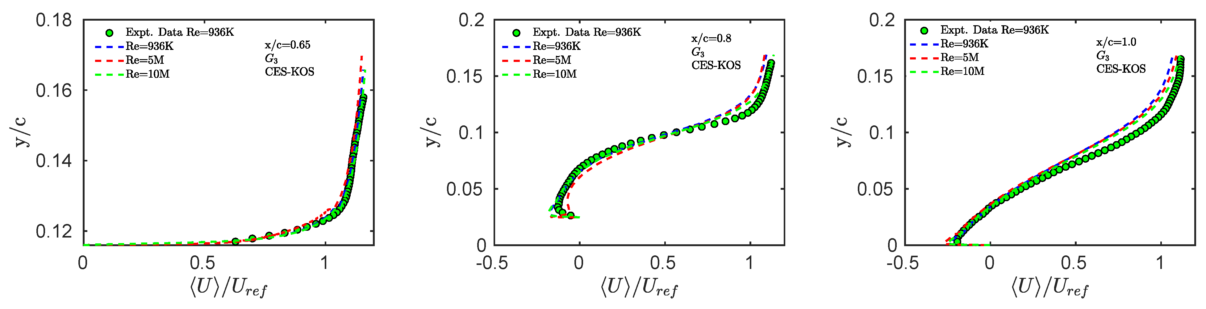
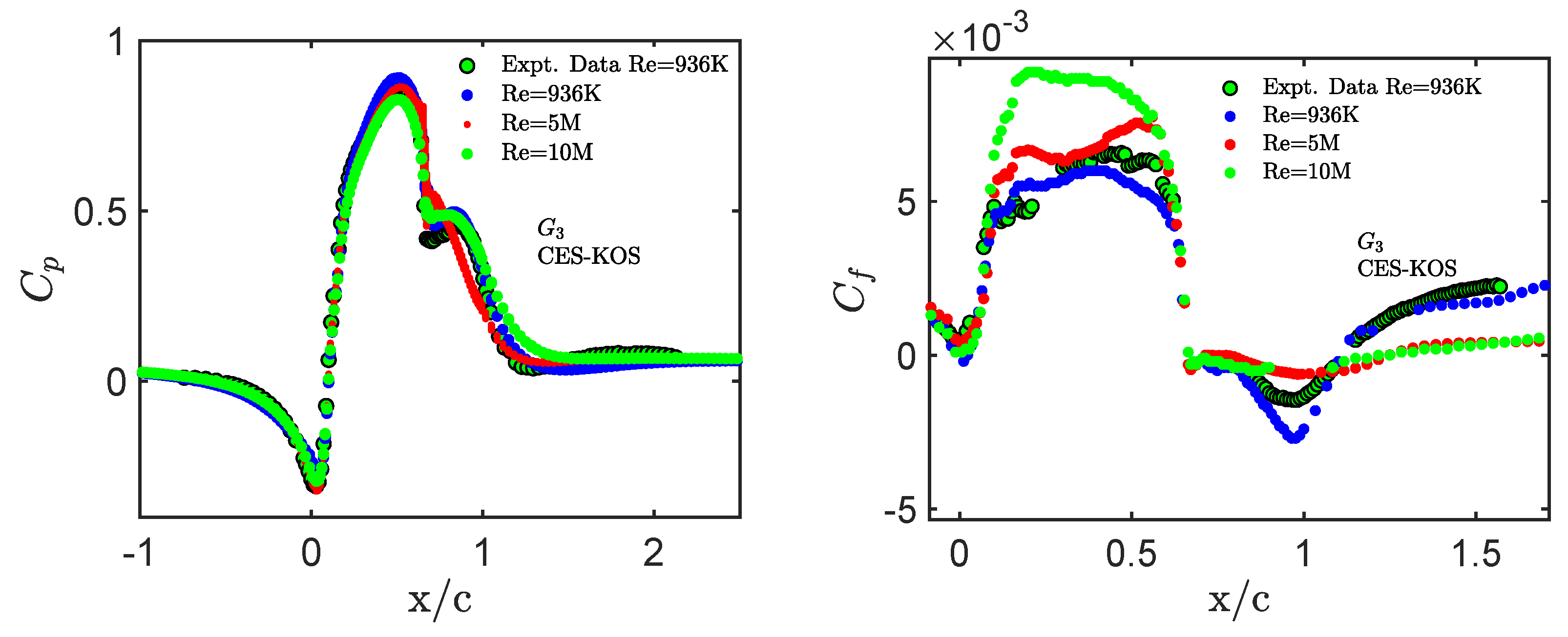
- The structural effects of increased on the mean velocity field are relatively small; there are only very minor variations. This speaks for the consideration of an range that is relatively close to an asymptotic regime. Correspondingly, the pressure coefficient distribution is little affected by increasing .
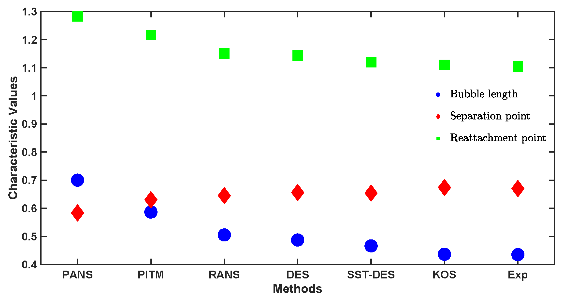
- On the other hand, the skin friction coefficient distribution and bubble length were identified as sensitive measures of Reynolds number dependence. Both are clearly affected by higher in response to an increased intensity of turbulent fluctuations and larger-scale structures in the flow.
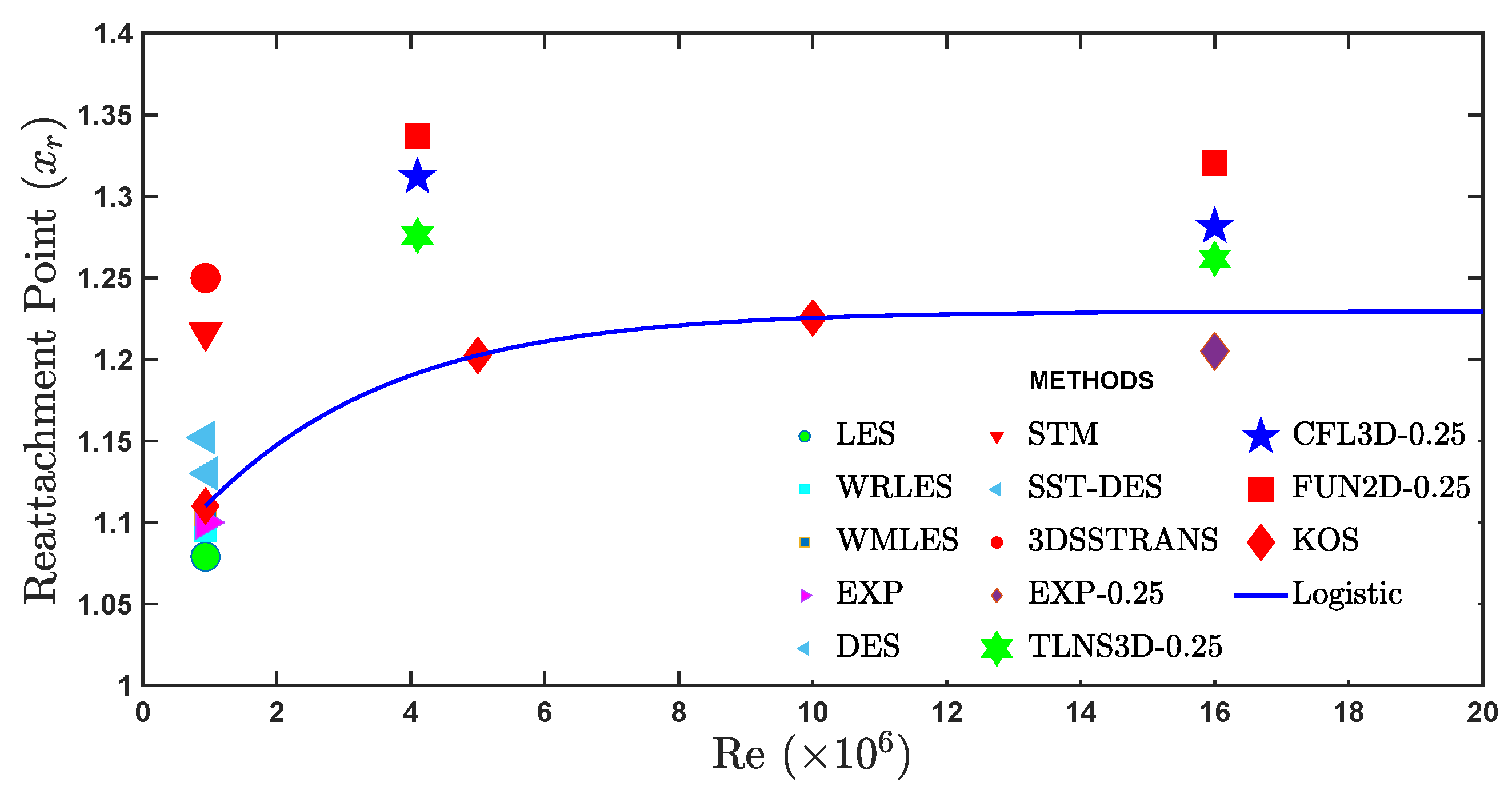
- Reattachment point predictions were used to specifically ask about the potential existence of an asymptotic regime for the flow considered. CES-KOS predictions confirm that there is an asymptotic regime. The M case is at least very close to this asymptotic regime. This conclusion is well supported by corresponding RANS predictions. This observation is in meaningful agreement with corresponding periodic hill flow studies indicating the existence of an asymptotic regime for M [20].
Author Contributions
Funding
Data Availability Statement
Acknowledgments
Conflicts of Interest
References
- Pope, S.B. Turbulent Flows; Cambridge University Press: Cambridge, UK, 2000. [Google Scholar]
- Sagaut, P. Large Eddy Simulation for Incompressible Flows: An Introduction; Springer: Berlin, Germany, 2002. [Google Scholar]
- Piomelli, U. Large-eddy simulation: Achievements and challenges. Prog. Aerosp. Sci. 1999, 35, 335–362. [Google Scholar] [CrossRef]
- Meneveau, C.; Katz, J. Scale-invariance and turbulence models for large-eddy simulation. Annu. Rev. Fluid Mech. 2000, 32, 1–32. [Google Scholar] [CrossRef]
- Heinz, S. A review of hybrid RANS-LES methods for turbulent flows: Concepts and applications. Prog. Aerosp. Sci. 2020, 114, 100597/1–100597/25. [Google Scholar] [CrossRef]
- Fröhlich, J.; Terzi, D.V. Hybrid LES/RANS methods for the simulation of turbulent flows. Prog. Aerosp. Sci. 2008, 44, 349–377. [Google Scholar] [CrossRef]
- Mockett, C.; Fuchs, M.; Thiele, F. Progress in DES for wall-modelled LES of complex internal flows. Comput. Fluids 2012, 65, 44–55. [Google Scholar] [CrossRef]
- Chaouat, B. The state of the art of hybrid RANS/LES modeling for the simulation of turbulent flows. Flow Turbul. Combust. 2017, 99, 279–327. [Google Scholar] [CrossRef]
- Menter, F.; Hüppe, A.; Matyushenko, A.; Kolmogorov, D. An overview of hybrid RANS–LES models developed for industrial CFD. Appl. Sci. 2021, 11, 2459. [Google Scholar] [CrossRef]
- Spalart, P.R. Detached-eddy simulation. Annu. Rev. Fluid Mech. 2009, 41, 181–202. [Google Scholar] [CrossRef]
- Shur, M.L.; Spalart, P.R.; Strelets, M.K.; Travin, A. A hybrid RANS-LES approach with delayed-DES and wall-modelled LES capabilities. Int. J. Heat Fluid Flow 2008, 29, 1638–1649. [Google Scholar] [CrossRef]
- Spalart, P.R.; Deck, S.; Shur, M.L.; Squires, K.D.; Strelets, M.K.; Travin, A. A new version of detached-eddy simulation, resistant to ambiguous grid densities. Theor. Comput. Fluid Dyn. 2006, 20, 181–195. [Google Scholar] [CrossRef]
- Menter, F.R.; Kuntz, M.; Langtry, R. Ten years of industrial experience with SST turbulence model. Turb. Heat Mass Transf. 2003, 4, 625–632. [Google Scholar]
- Bose, S.T.; Park, G. Wall-modeled large eddy simulation for complex turbulent flow. Annu. Rev. Fluid Mech. 2018, 50, 535–561. [Google Scholar] [CrossRef] [PubMed]
- Larsson, J.; Kawai, S.; Bodart, J.; Bermejo-Moreno, I. Large eddy simulation with modeled wall-stress: Recent progress and future directions. Mech. Eng. Rev. 2016, 3, 15–00418/1–15–00418/23. [Google Scholar] [CrossRef]
- Iyer, P.S.; Malik, M.R. Wall-modeled large eddy simulation of flow over a wallmounted hump. In Proceedings of the 2016 AIAA Aerospace Sciences Meeting, AIAA SciTech Forum, Washington, DC, USA, 13–17 June 2016; AIAA Paper 16-3186. pp. 1–22. [Google Scholar]
- Dong, T.; Minelli, G.; Wang, J.; Liang, X.; Krajnović, S. Numerical investigation of a high-speed train underbody flows: Studying flow structures through large-eddy simulation and assessment of steady and unsteady Reynolds-averaged Navier–Stokes and improved delayed detached eddy simulation performance. Phys. Fluids 2022, 34, 015126. [Google Scholar] [CrossRef]
- Haering, S.W.; Oliver, T.A.; Moser, R.D. Active model split hybrid RANS/LES. Phys. Review Fluids 2022, 7, 014603. [Google Scholar] [CrossRef]
- Heinz, S. The large eddy simulation capability of Reynolds-averaged Navier-Stokes equations: Analytical results. Phys. Fluids 2019, 31, 021702/1–021702/6. [Google Scholar] [CrossRef]
- Heinz, S.; Mokhtarpoor, R.; Stoellinger, M.K. Theory-Based Reynolds-Averaged Navier-Stokes Equations with Large Eddy Simulation Capability for Separated Turbulent Flow Simulations. Phys. Fluids 2020, 32, 065102/1–065102/20. [Google Scholar] [CrossRef]
- Heinz, S. The Continuous Eddy Simulation Capability of Velocity and Scalar Probability Density Function Equations for Turbulent Flows. Phys. Fluids 2021, 33, 025107/1–025107/13. [Google Scholar] [CrossRef]
- Heinz, S. Remarks on Energy Partitioning Control in the PITM Hybrid RANS/LES Method for the Simulation of Turbulent Flows. Flow, Turb. Combust. 2022, 108, 927–933. [Google Scholar] [CrossRef]
- Heinz, S. Theory-Based Mesoscale to Microscale Coupling for Wind Energy Applications. Appl. Math. Model. 2021, 98, 563–575. [Google Scholar] [CrossRef]
- Heinz, S. Minimal error partially resolving simulation methods for turbulent flows: A dynamic machine learning approach. Phys. Fluids 2022, 34, 051705/1–051705/7. [Google Scholar] [CrossRef]
- Heinz, S. A Mathematical Solution to the Computational Fluid Dynamics (CFD) Dilemma. Mathematics 2023, 11, 3199. [Google Scholar] [CrossRef]
- Mokhtarpoor, R.; Heinz, S.; Stoellinger, M. Dynamics unified RANS-LES simulations of high Reynolds number separated flows. Phys. Fluids 2016, 28, 095101/1–095101/36. [Google Scholar] [CrossRef]
- Openfoam Documentation. Technical Report. 2009. Available online: www.openfoam.org (accessed on 1 January 2020).
- Rodi, W. On the simulation of turbulent flow past bluff bodies. J. Wind Eng. Ind. Aerodyn. 1993, 46, 3–19. [Google Scholar] [CrossRef]
- Lin, S.J.; Chao, W.C.; Sud, Y.C.; Walker, G.K. A class of the van Leer-type transport schemes and its application to the moisture transport in a general circulation model. Mon. Weather Rev. 1994, 122, 1575–1593. [Google Scholar] [CrossRef]
- Issa, R.I. Solution of the implicitly discretised fluid flow equations by operator-splitting. J. Comput. Phys. 1986, 62, 40–65. [Google Scholar] [CrossRef]
- Arany, I. The preconditioned conjugate gradient method with incomplete factorization preconditioners. Comput. Math. Appl. 1996, 31, 1–5. [Google Scholar] [CrossRef]
- Seifert, A.; Pack, L. Active flow separation control on wall-mounted hump at high Reynolds numbers. AIAA J. 2002, 40, 1362–1372. [Google Scholar] [CrossRef]
- Greenblatt, D.; Paschal, K.B.; Yao, C.-S.; Harris, J.; Schaeffler, N.W.; Washburn, A.E. Experimental Investigation of Separation Control Part 1: Baseline and Steady Suction. AIAA J. 2006, 44, 2820–2830. [Google Scholar] [CrossRef]
- Uzun, A.; Malik, M. Large-Eddy Simulation of flow over a wall-mounted hump with separation and reattachment. AIAA J. 2018, 56, 715–730. [Google Scholar] [CrossRef]
- You, D.; Wang, M.; Moin, P. Large-eddy simulation of flow over a wall-mounted hump with separation control. AIAA J. 2006, 44, 2571–2577. [Google Scholar] [CrossRef]
- Montorfano, A.; Piscaglia, F.; Ferrari, G. Inlet boundary conditions for incompressible LES: A comparative study. Math. Comput. Model. 2013, 57, 1640–1647. [Google Scholar] [CrossRef]
- Lund, T.S.; Wu, X.; Squires, K. Generation of turbulent inflow data for spatially developing boundary layer simulations. J. Comput. Phys. 1998, 140, 233–258. [Google Scholar] [CrossRef]
- Simens, M.; Jiménez, J.; Hoyas, S. A high-resolution code for turbulent boundary layers. J. Comput Phys. 2009, 228, 4218–4231. [Google Scholar] [CrossRef]
- Capizzano, F.; Catalano, P.; Marongiu, C.; Vitagliano, P.L. U-RANS modelling of turbulent flows controlled by synthetic jets. In Proceedings of the 35th AIAA Fluid Dynamics Conference and Exhibit, Toronto, ON, Canada, 6–9 June 2005; AIAA Paper 05-5015. pp. 1–20. [Google Scholar]
- Viken, S.; Vatsa, V.; Rumsey, C.; Carpenter, M. Flow control analysis on the hump model with RANS tools. AIAA J. 2003, 218. [Google Scholar] [CrossRef]
- Krishnan, V.; Squires, K.D.; Forsythe, J.R. Prediction of separated flow characteristics over a hump using RANS and DES. In Proceedings of the 2nd AIAA Flow Control Conference, Portland, OR, USA, 28 June–1 July 2004; p. 2224. [Google Scholar]
- Lardeau, S.; Billard, C.F. Development of an elliptic-blending lag model for industrial applications. In Proceedings of the 2016 AIAA Aerospace Sciences Meeting, AIAA SciTech Forum, San Diego, CA, USA, 4–8 January 2016; AIAA Paper 16-1600. pp. 1–17. [Google Scholar]
- Probst, A.; Schwamborn, D.; Garbaruk, A.; Guseva, M.; Strelets, M.; Travin, A. Evaluation of grey area mitigation tools within zonal and non-zonal RANS-LES approaches in flows with pressure induced separation. Int. J. Heat Fluid Flow 2017, 68, 237–247. [Google Scholar] [CrossRef]
- Ren, X.; Su, H.; Yu, H.H.; Yan, Z. Wall-Modeled Large Eddy Simulation and Detached Eddy Simulation of Wall-Mounted Separated Flow via OpenFOAM. Aerospace 2022, 9, 759. [Google Scholar] [CrossRef]
- Avdis, A.; Lardeau, S.; Leschziner, M. Large eddy simulation of separated flow over a two-dimensional hump with and without control by means of a synthetic slotjet. Flow Turbul. Combust. 2009, 83, 343–370. [Google Scholar] [CrossRef]
- Uzun, A.; Malik, M.R. Wall-resolved large-eddy simulation of flow separation over NASA wall-mounted hump. In Proceedings of the 55th AIAA Aerospace Sciences Meeting, Grapevine, TX, USA, 9–13 January 2017; p. AIAA Paper 17–0538. [Google Scholar]
- Yang, X.I.A.; Griffin, K.P. Grid-point and time-step requirements for direct numerical simulation and large-eddy simulation. Phys. Fluids 2021, 33, 015108. [Google Scholar] [CrossRef]
- Lei, D.; Yang, H.; Zheng, Y.; Gao, Q.; Jin, X. A Modified Shielding and Rapid Transition DDES Model for Separated Flows. Entropy 2023, 25, 613. [Google Scholar] [CrossRef]
- Heinz, S.; Heinz, J.; Brant, J.A. Mass Transport in Membrane Systems: Flow Regime Identification by Fourier Analysis. Fluids 2022, 7, 369. [Google Scholar]
- Radoslav Bozinoski, a.R.L.D. A DES Procedure Applied to a Wall-Mounted Hump. Int. J. Aerosp. Eng. 2012, 2012, 149461. [Google Scholar]
- Woodruff, S. Model-invariant hybrid computations of separated flows for RCA standard test cases. In Proceedings of the 2016 AIAA SciTech Forum, San Diego, CA, USA, 4–8 January 2016; AIAA Paper 16-1559. pp. 1–19. [Google Scholar]
- Kähler, C.J.; Scharnowski, S.; Cierpka, C. Highly resolved experimental results of the separated flow in a channel with streamwise periodic constrictions. J. Fluid Mech. 2016, 796, 257–284. [Google Scholar] [CrossRef]
- Heinz, S. On mean flow universality of turbulent wall flows. I. High Reynolds number flow analysis. J. Turbul. 2018, 19, 929–958. [Google Scholar]
- Heinz, S. On mean flow universality of turbulent wall flows. II. Asymptotic flow analysis. J. Turbul. 2019, 20, 174–193. [Google Scholar] [CrossRef]
- Advanced Research Computing Center. Mount Moran: IBM System X Cluster; University of Wyoming: Laramie, WY, USA, 2018; Available online: http://n2t.net/ark:/85786/m4159c (accessed on 4 December 2018).
- Advanced Research Computing Center. Teton Computing Environment, Intel x86_64 Cluster; University of Wyoming: Laramie, WY, USA, 2018. [Google Scholar] [CrossRef]


| Model | CES Hybrid Equations | Mode Control |
|---|---|---|
| CES-KOS: | ||
| CES-KOK: | ||
| CES-KOKU: |
| Run | Grid | Grid Points | Resolution | Inflow (Generation) Plane | Min. Wall Spacing | |
|---|---|---|---|---|---|---|
| Coarse | 480 K | 323 | plane mapping, | 0.0001 | 1.25 | |
| Medium | 960 K | plane mapping, | 0.00001 | 0.75 | ||
| Fine | 1.7 million | plane mapping, | 0.000005 | 0.25 | ||
| Very fine | 3.9 million | plane mapping, | 0.000001 | 0.2 |
| Methods | Separation Location () | Reattachment Location () | Bubble Length | Error in Bubble LengthPrediction (%) |
|---|---|---|---|---|
| Exp. [33] | 0.435 | – | ||
| CES-KOS– | 0.6642 | 1.135 | 0.4708 | 8.2 |
| CES-KOS– | 0.6669 | 1.1144 | 0.4475 | 2.9 |
| CES-KOS– | 0.6737 | 1.1100 | 0.4363 | 0.3 |
| CES-KOS– | 0.6680 | 1.1000 | 0.432 | 0.7 |
| CES-KOK– | 0.6752 | 1.1333 | 0.4581 | 5.3 |
| Fluc. | |||
|---|---|---|---|
| u | |||
| v | |||
| w |
| Methods | Separation Location () | Reattachment Location () | Bubble Length | Error in Bubble Length Prediction (%) |
|---|---|---|---|---|
| Exp. [33] | 0.435 | – | ||
| CES-KOS– | 0.6737 | 1.1100 | 0.4363 | 0.3 |
| RANS– | 0.645 | 1.150 | 0.505 | 16.1 |
| RANS (Lardeau and Billard [42]) | – | 1.188–1.305 | – | – |
| URANS (Capizzano et al. [39]) | – | 1.25 | – | – |
| PANS- | 0.5833 | 1.2833 | 0.70 | 60.9 |
| PITM- | 0.6301 | 1.2166 | 0.5865 | 34.8 |
| DES (Probst et al. [43]) | 0.656 | 1.143 | 0.487 | 11.95 |
| SST-DES (Ren et al. [44]) | 0.654 | 1.12 | 0.466 | 7.13 |
| Methods | Separation Location () | Reattachment Location () | Bubble Length | Error in Bubble Length Prediction (%) |
|---|---|---|---|---|
| Exp. [33] | 0.435 | – | ||
| CES-KOS– | 0.6737 | 1.1100 | 0.4363 | 0.3 |
| LES- | 0.6710 | 1.1018 | 0.4308 | 1.7 |
| iLES (Avdis et al. [45]) | 0.658 | 1.079 | 0.421 | 3.2 |
| WRLES (Uzun and Malik [34,46]) | 0.659 | 1.095 | 0.436 | 0.23 |
| WMLES (Iyer and Malik [16]) | 0.637–0.655 | 1.035–1.105 | 0.398– 0.45 | 3.4–8.5 |
| Methods | N | ||
|---|---|---|---|
| KOS | 23,097 | ||
| WRLES | |||
| WMLES | |||
| DES | 72,375 |
| Cases | Re | Separation Location () | Reattachment () | Bubble Length | Error in Bubble Length Prediction (%) |
|---|---|---|---|---|---|
| Exp. [33] | K | 0.4350 | – | ||
| K | 0.6737 | 1.1100 | 0.4363 | 0.3 | |
| M | 0.6713 | 1.2167 | 0.5454 | – | |
| M | 0.6641 | 1.2165 | 0.5524 | – | |
| K | 0.6680 | 1.100 | 0.4320 | 0.7 | |
| M | 0.6725 | 1.2025 | 0.5300 | – | |
| M | 0.6812 | 1.2245 | 0.5433 | – |
| Methods | Reference | Re | Reattachment Point () |
|---|---|---|---|
| Exp. | Greenblatt et al. [33] | 936 K | |
| RANS | Lardeau & Billard [42] | 936 K | 1.3050 |
| LES | Avdis et al. [45] | 936 K | 1.0790 |
| LES (WRLES) | Uzun and Malik [46] | 936 K | 1.0950 |
| Hybrid (WMLES) | Iyer and Malik [16] | 936 K | 1.035–1.1050 |
| Hybrid (DES) | Probst et al. [43], Radoslav & Roger [50] | 936 K | 1.1520, 1.1050 |
| Hybrid (SST-DES) | Ren et al. [44] | 936 K | 1.1200 |
| Hybrid (STM) | Woodruff [51] | 936 K | 1.0800–1.1900 |
| Hybrid (KOS) | (936 K, 5 M, 10 M) | (1.1100, 1.2025, 1.2255) | |
| Exp. | Vatsa et al. [40] | 4.2 M | |
| URANS (FUN2D) | Vatsa et al. [40] | (4.2 M, 16 M) | (1.3330, 1.3100) |
| RANS (TLNS3D) | Vatsa et al. [40] | (4.2 M, 16 M) | (1.2700, 1.2550) |
| RANS (CFL3D) | Vatsa et al. [40] | (4.2 M, 16 M) | (1.3040, 1.2830) |
Disclaimer/Publisher’s Note: The statements, opinions and data contained in all publications are solely those of the individual author(s) and contributor(s) and not of MDPI and/or the editor(s). MDPI and/or the editor(s) disclaim responsibility for any injury to people or property resulting from any ideas, methods, instructions or products referred to in the content. |
© 2024 by the authors. Licensee MDPI, Basel, Switzerland. This article is an open access article distributed under the terms and conditions of the Creative Commons Attribution (CC BY) license (https://creativecommons.org/licenses/by/4.0/).
Share and Cite
Fagbade, A.; Heinz, S. Continuous Eddy Simulation vs. Resolution-Imposing Simulation Methods for Turbulent Flows. Fluids 2024, 9, 22. https://doi.org/10.3390/fluids9010022
Fagbade A, Heinz S. Continuous Eddy Simulation vs. Resolution-Imposing Simulation Methods for Turbulent Flows. Fluids. 2024; 9(1):22. https://doi.org/10.3390/fluids9010022
Chicago/Turabian StyleFagbade, Adeyemi, and Stefan Heinz. 2024. "Continuous Eddy Simulation vs. Resolution-Imposing Simulation Methods for Turbulent Flows" Fluids 9, no. 1: 22. https://doi.org/10.3390/fluids9010022