
A Numerical Study on the Erythrocyte Flow Path in I-Shaped Pillar DLD Arrays

Abstract
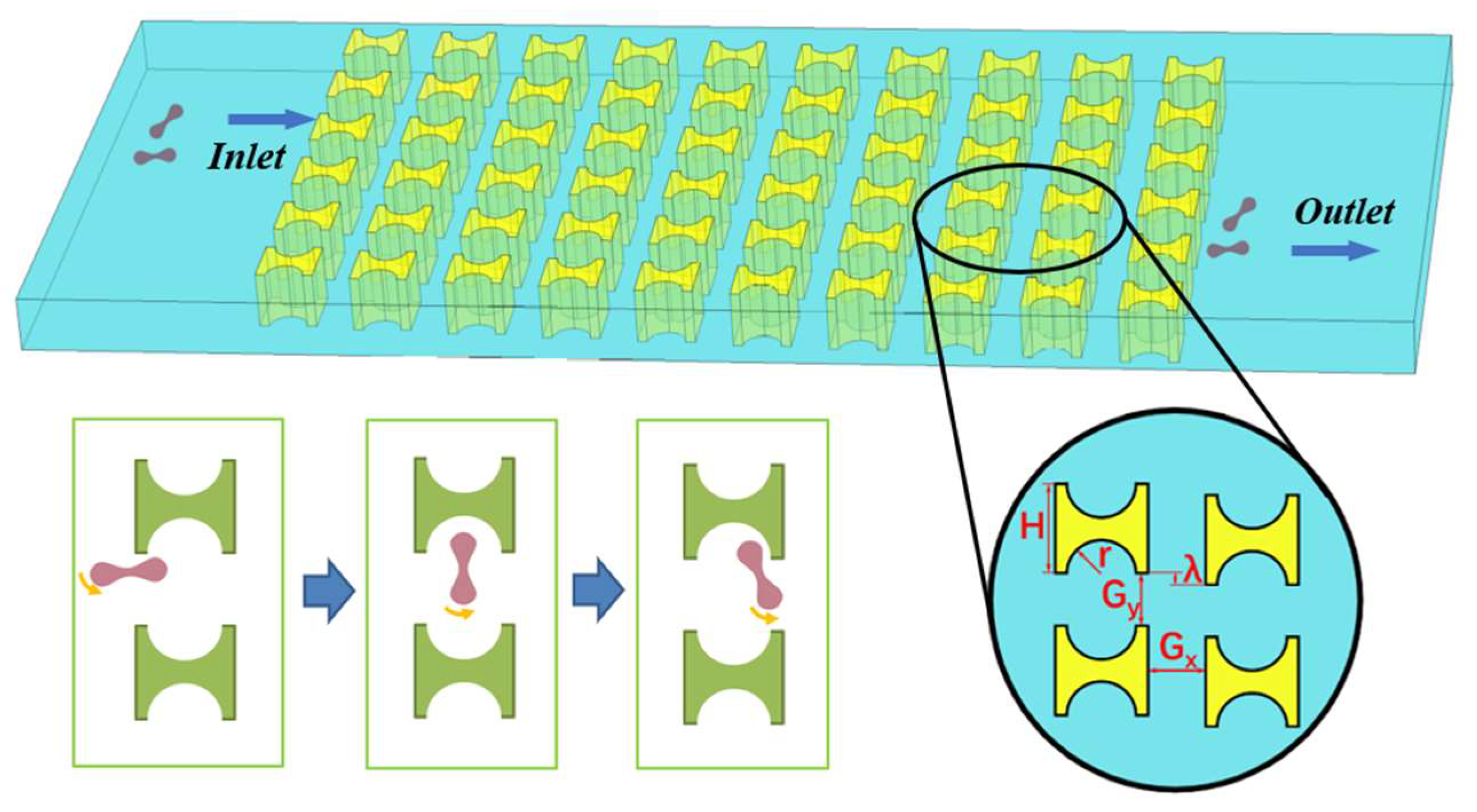
:1. Introduction
2. Calculation Method
2.1. Fluid Flow Solver
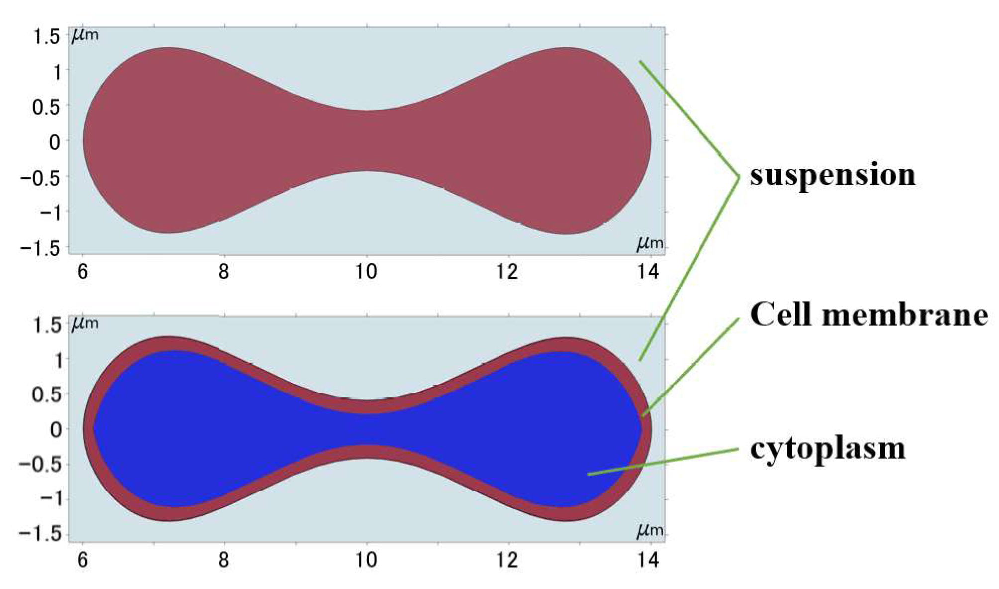
2.2. Erythrocyte Structure Solver
2.3. Coupling of Fluid and Erythrocyte Solvers
3. Model Verification and Flow Simulation
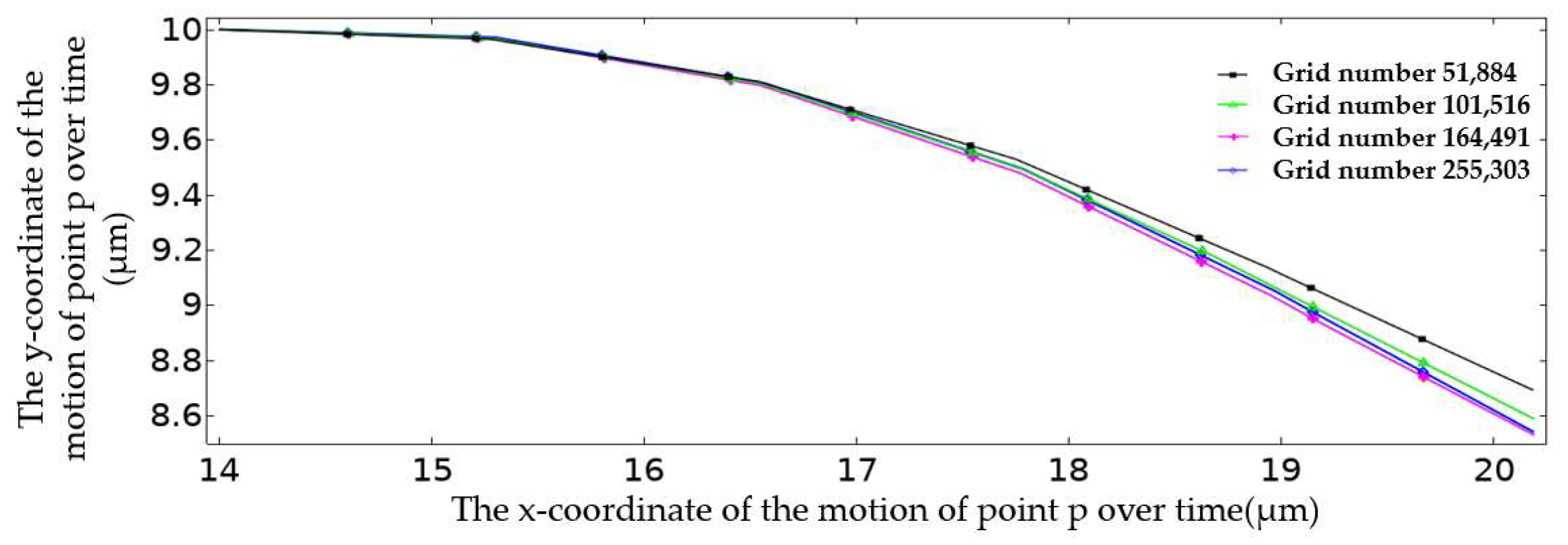
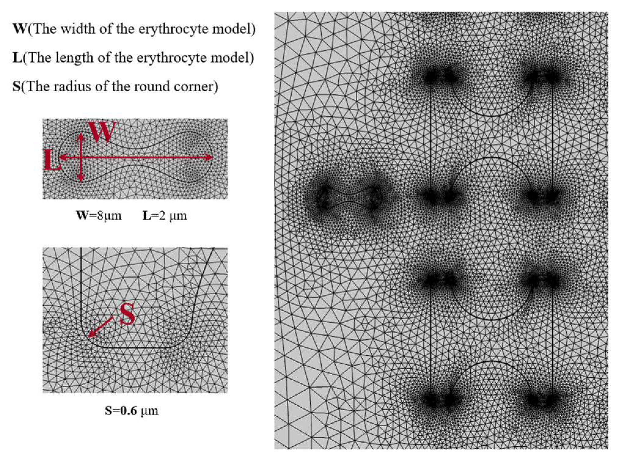
3.1. Verification of Simulation Accuracy
3.2. Experimental Scheme Design
4. Analysis of Simulation Results
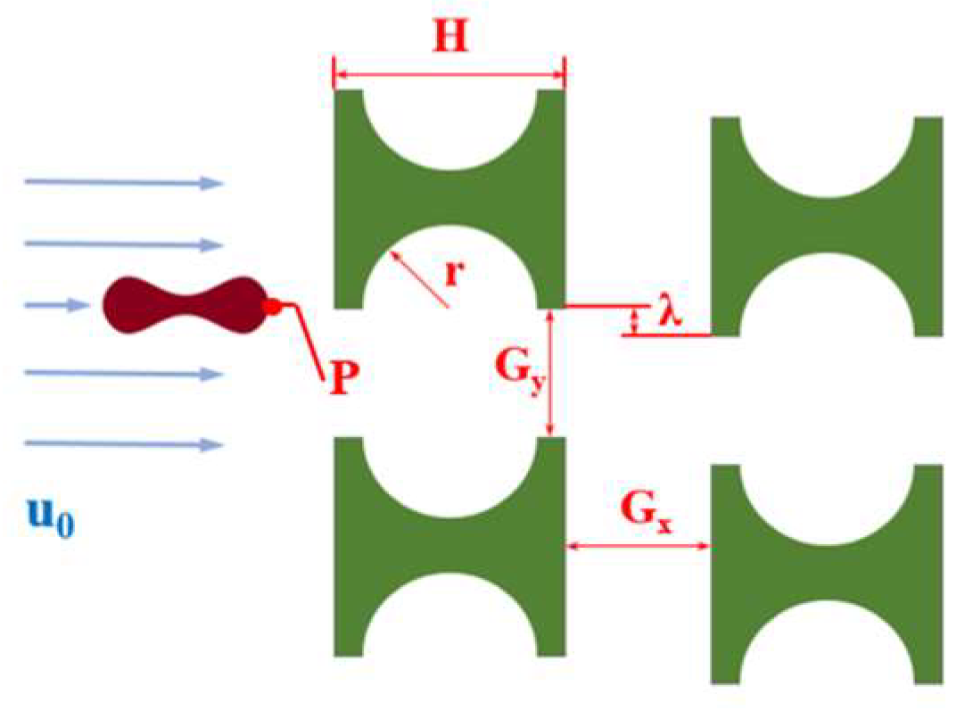
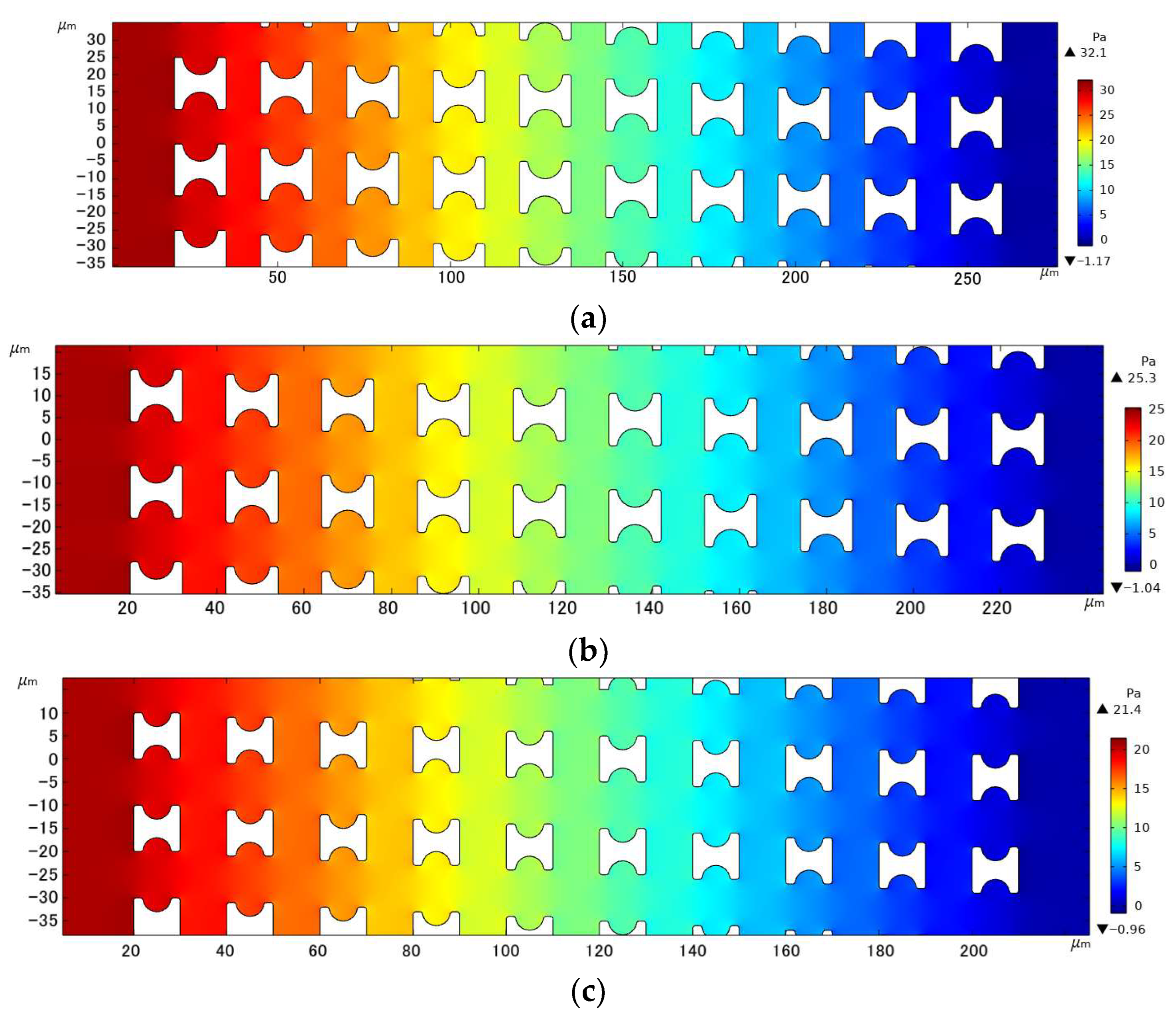
4.1. Effects of Pillar Shape on Pressure Distribution within the Array
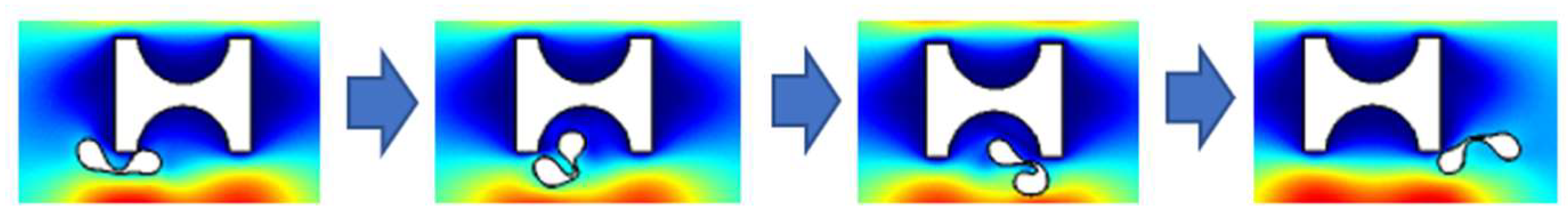
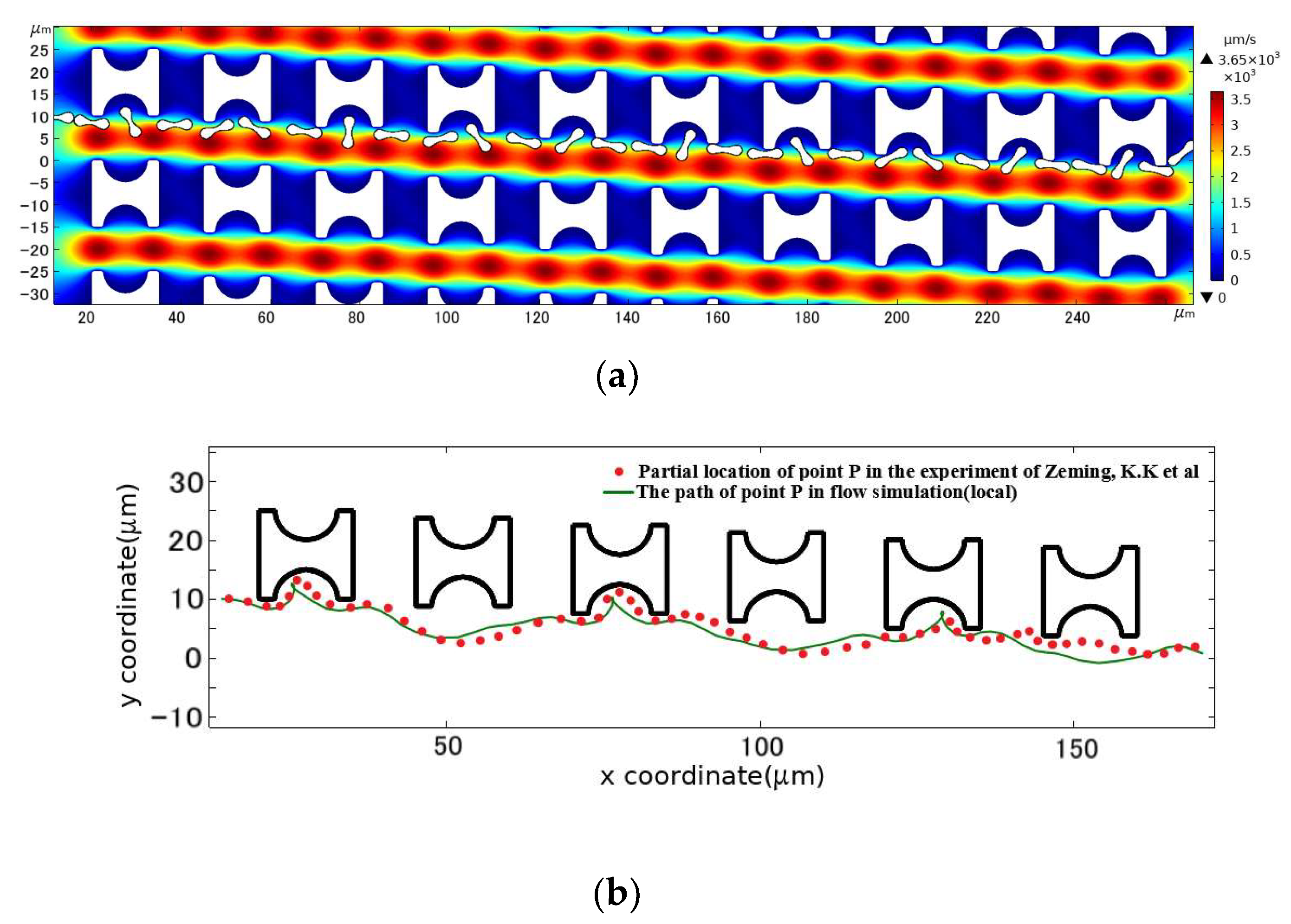
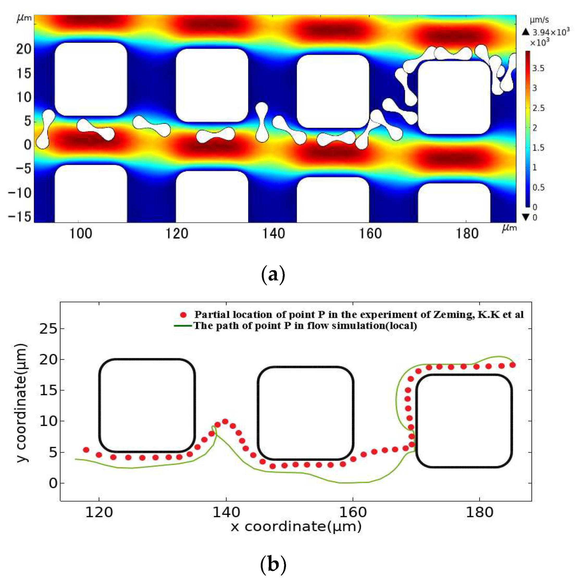
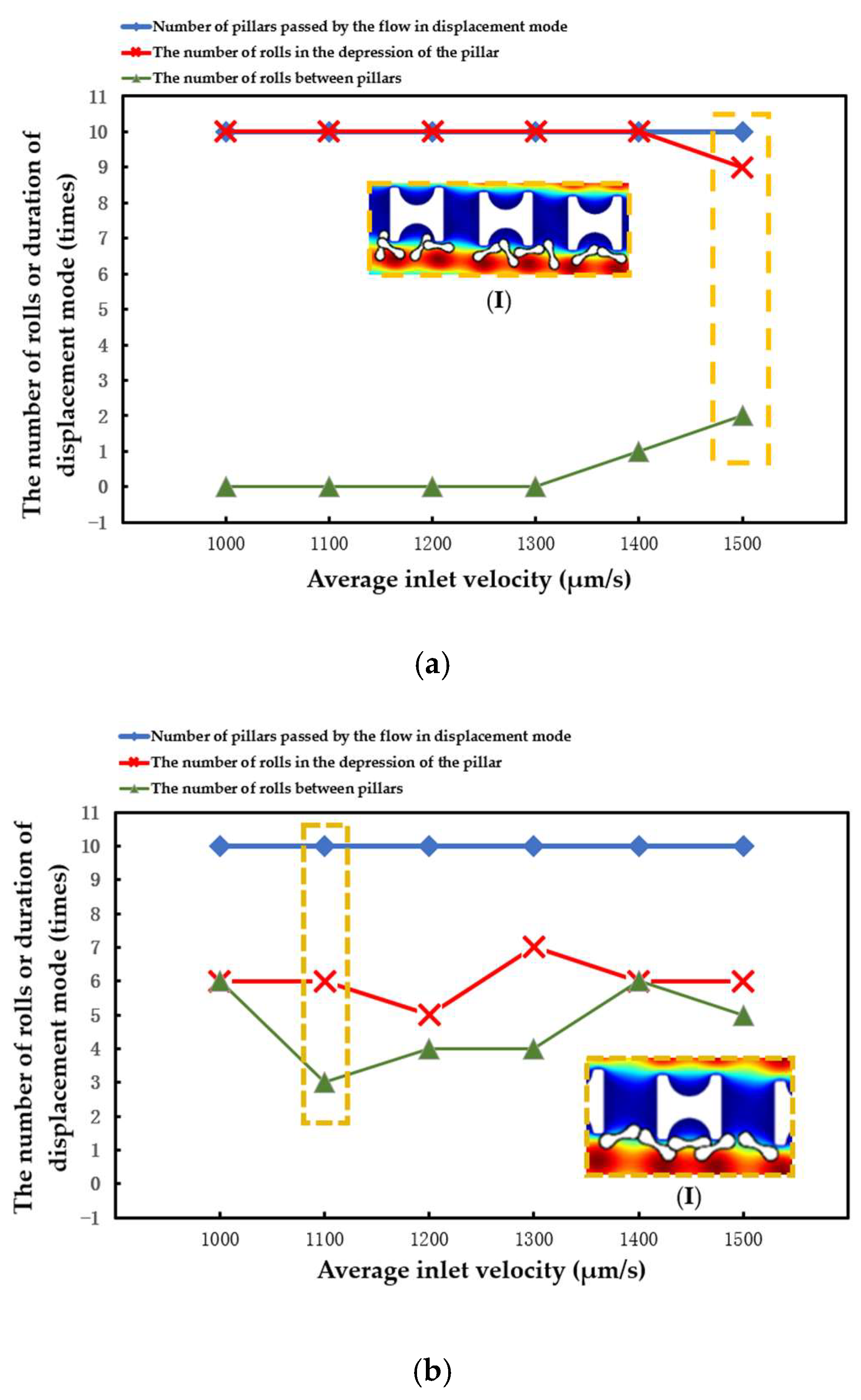
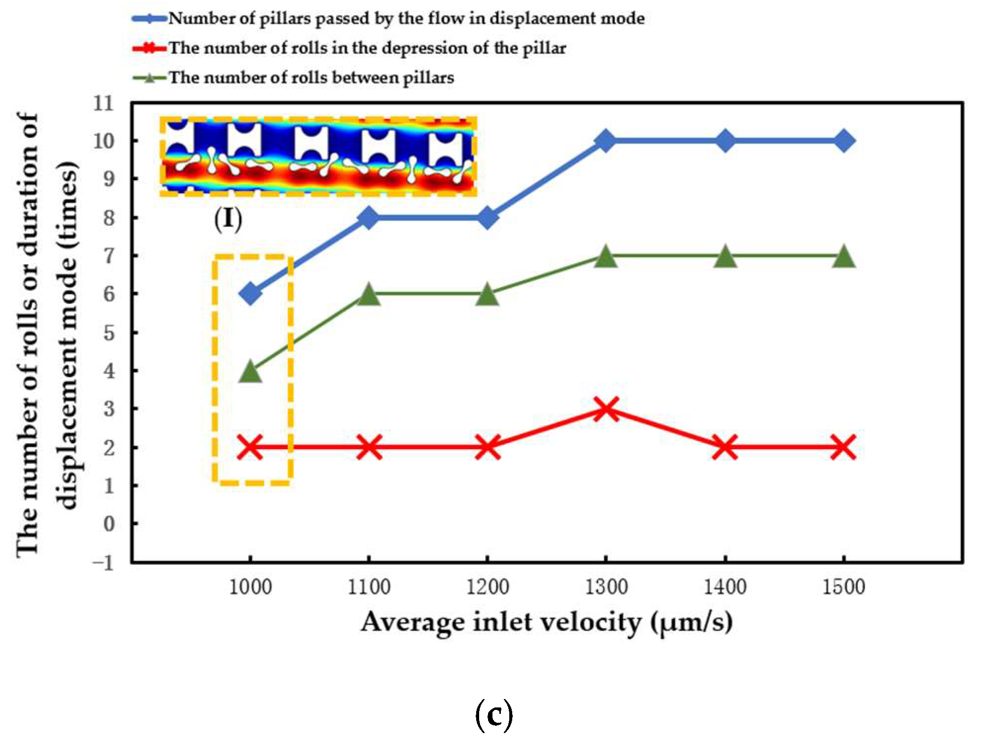
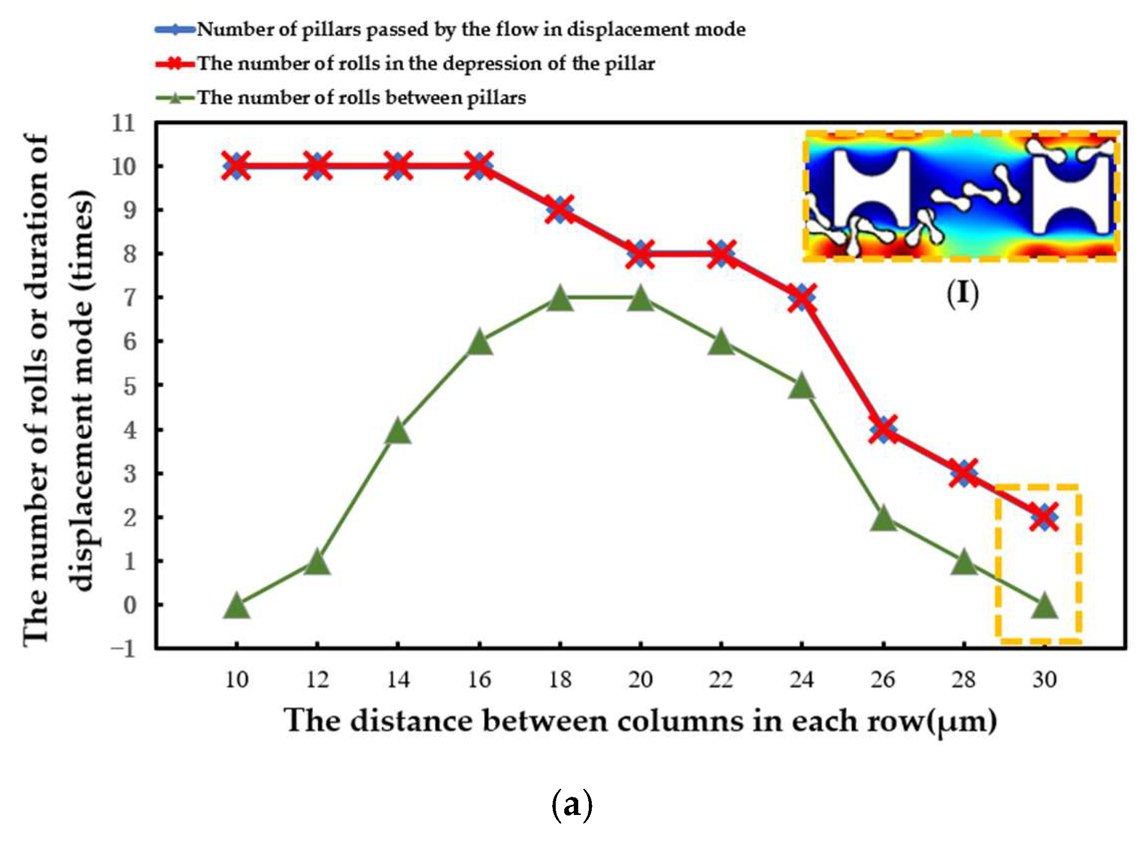
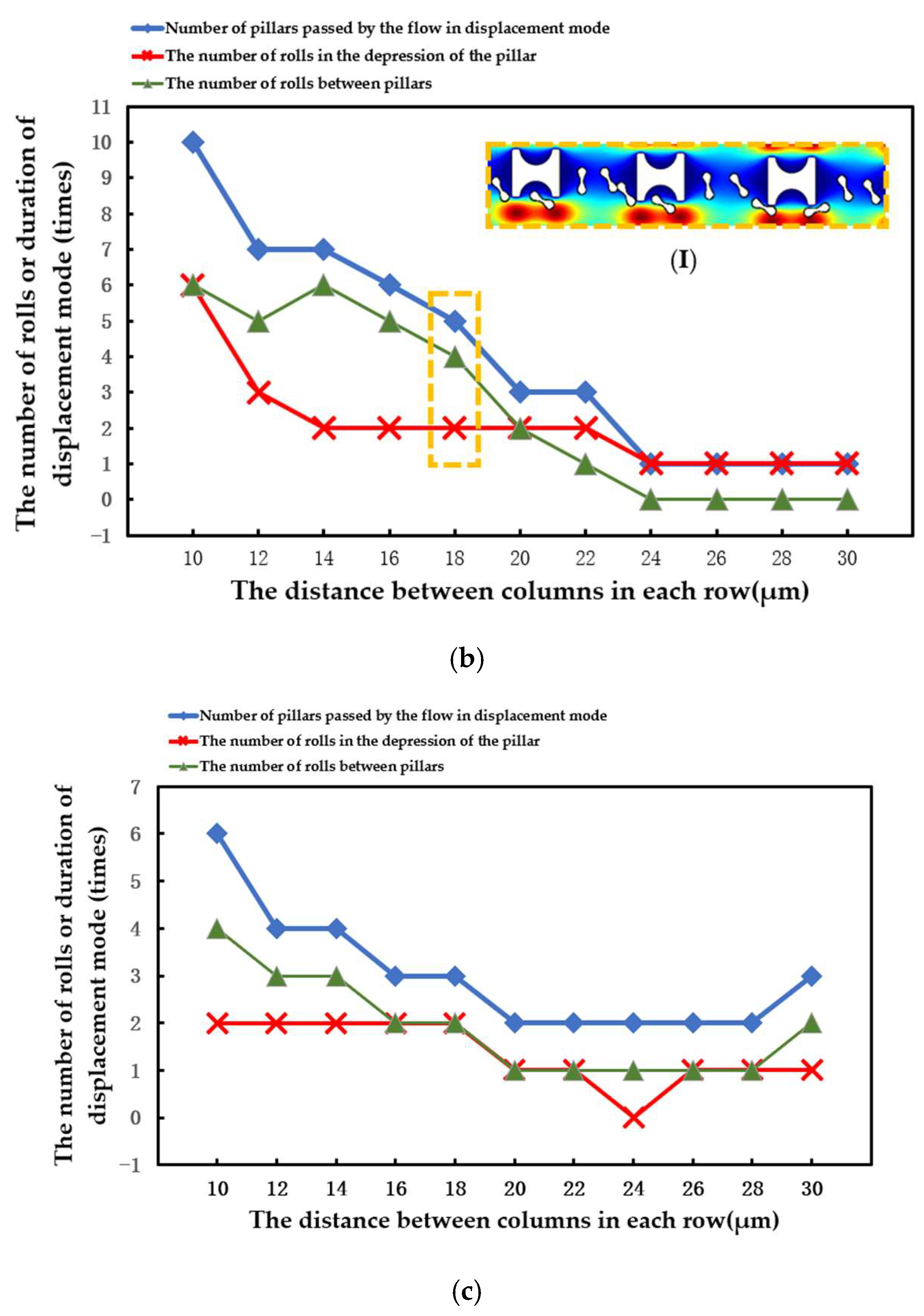
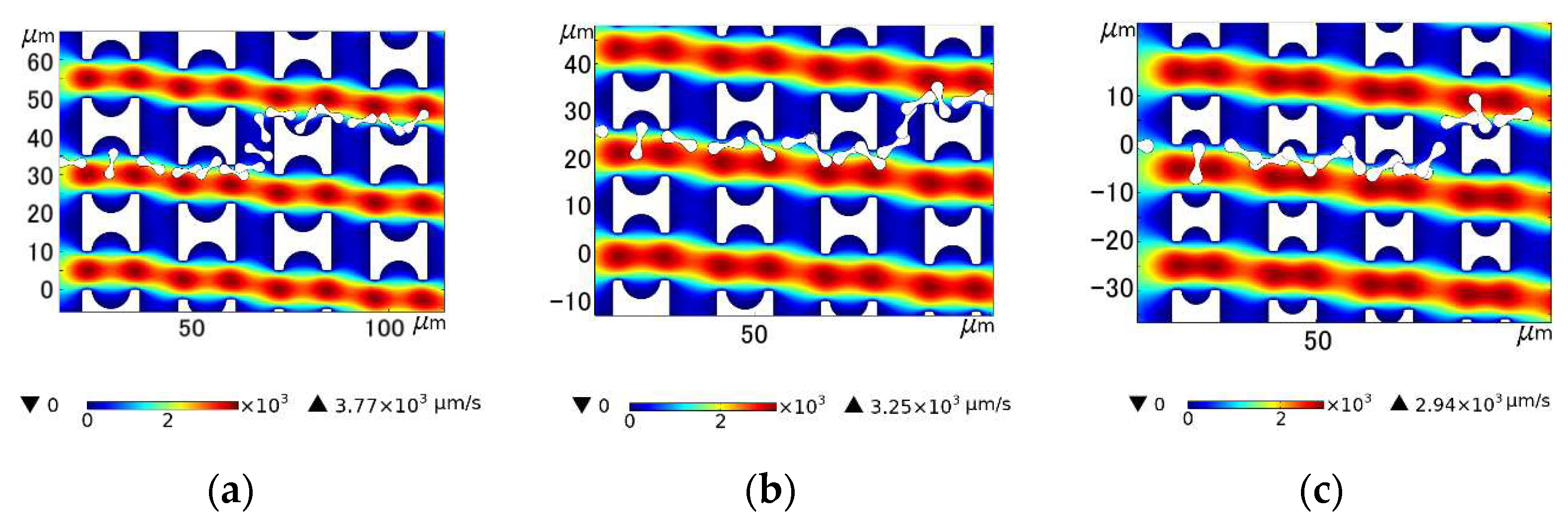
4.2. Movement of Erythrocyte Models in Each Array
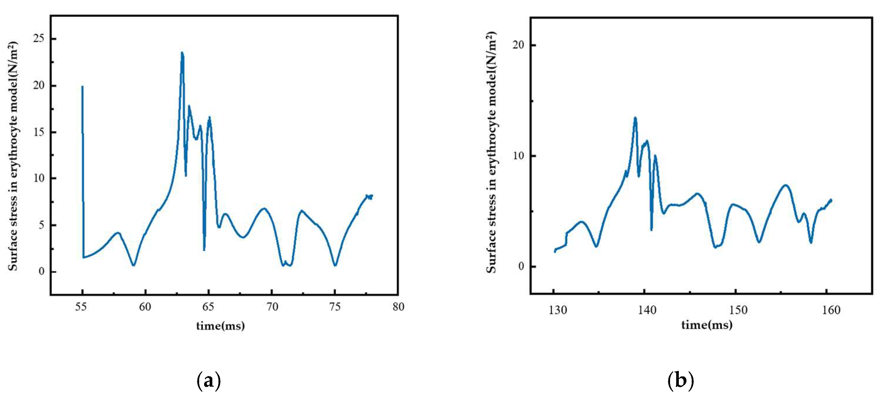
4.3. Surface Stress in the Erythrocyte Model
5. Conclusions
Author Contributions
Funding
Conflicts of Interest
References
- Tsubota, K.-I.; Wada, S.; Yamaguchi, T. Particle method for computer simulation of red blood cell motion in blood flow. Comput. Methods Programs Biomed. 2006, 83, 139–146. [Google Scholar] [CrossRef] [PubMed]
- Mendez, S.; Chnafa, C.; Gibaud, E.; Sigueenza, J.; Moureau, V.; Nicoud, F. YALES2BIO: A Computational Fluid Dynamics Software Dedicated to the Prediction of Blood Flows in Biomedical Devices. In Proceedings of the 5th International Conference on the Development of Biomedical Engineering in Vietnam, Ho Chi Minh City, Vietnam, 16–18 June 2015; pp. 7–10. [Google Scholar]
- Ju, M.; Ye, S.S.; Namgung, B.; Cho, S.; Low, H.T.; Leo, H.L.; Kim, S. A review of numerical methods for red blood cell flow simulation. Comput. Methods Biomech. Biomed. Eng. 2015, 18, 130–140. [Google Scholar] [CrossRef]
- Bizjak, D.A.; John, L.; Matits, L.; Uhl, A.; Schulz, S.V.W.; Schellenberg, J.; Peifer, J.; Bloch, W.; Weiss, M.; Gruner, B.; et al. SARS-CoV-2 Altered Hemorheological and Hematological Parameters during One-Month Observation Period in Critically Ill COVID-19 Patients. Int. J. Mol. Sci. 2022, 23, 15332. [Google Scholar] [CrossRef] [PubMed]
- Niesor, E.J.; Nader, E.; Perez, A.; Lamour, F.; Benghozi, R.; Remaley, A.; Thein, S.L.; Connes, P. Red Blood Cell Membrane Cholesterol May Be a Key Regulator of Sickle Cell Disease Microvascular Complications. Membranes 2022, 12, 1134. [Google Scholar] [CrossRef] [PubMed]
- Hareendranath, S.; Sathian, S.P. Dynamic response of red blood cells in health and disease. Soft Matter 2023, 19, 1219–1230. [Google Scholar] [CrossRef]
- Laxmi, V.; Joshi, S.S.; Agrawal, A. Extracting white blood cells from blood on microfluidics platform: A review of isolation techniques and working mechanisms. J. Micromech. Microeng. 2022, 32, 053001. [Google Scholar] [CrossRef]
- Salafi, T.; Zhang, Y.; Zhang, Y. A Review on Deterministic Lateral Displacement for Particle Separation and Detection. Nano-Micro Lett. 2019, 11, 77. [Google Scholar] [CrossRef]
- Hochstetter, A.; Vernekar, R.; Austin, R.H.; Becker, H.; Beech, J.P.; Fedosov, D.A.; Gompper, G.; Kim, S.C.; Smith, J.T.; Stolovitzky, G.; et al. Deterministic Lateral Displacement: Challenges and Perspectives. ACS Nano 2020, 14, 10784–10795. [Google Scholar] [CrossRef]
- Xavier, M.; Holm, S.H.; Beech, J.P.; Spencer, D.; Tegenfeldt, J.O.; Oreffo, R.O.C.; Morgan, H. Label-free enrichment of primary human skeletal progenitor cells using deterministic lateral displacement. Lab Chip 2019, 19, 513–523. [Google Scholar] [CrossRef]
- Rahmati, M.; Chen, X.L. Separation of circulating tumor cells from blood using dielectrophoretic DLD manipulation. Biomed. Microdevices 2021, 23, 49. [Google Scholar] [CrossRef]
- Wang, Y.P.; Gao, Y.F.; Song, Y.J. Microfluidics-Based Urine Biopsy for Cancer Diagnosis: Recent Advances and Future Trends. ChemMedChem 2022, 17, e202200422. [Google Scholar] [CrossRef] [PubMed]
- Tang, H.; Niu, J.; Pan, X.; Jin, H.; Lin, S.; Cui, D. Topology optimization based deterministic lateral displacement array design for cell separation. J. Chromatogr. A 2022, 1679, 463384. [Google Scholar] [CrossRef] [PubMed]
- Zeming, K.K.; Ranjan, S.; Zhang, Y. Rotational separation of non-spherical bioparticles using I-shaped pillar arrays in a microfluidic device. Nat. Commun. 2013, 4, 1625. [Google Scholar] [CrossRef]
- Ranjan, S.; Zeming, K.K.; Jureen, R.; Fisher, D.; Zhang, Y. DLD pillar shape design for efficient separation of spherical and non-spherical bioparticles. Lab Chip 2014, 14, 4250–4262. [Google Scholar] [CrossRef] [PubMed]
- Jiang, D.; Liu, S.W.; Tang, W.L. Fabrication and Manipulation of Non-Spherical Particles in Microfluidic Channels: A Review. Micromachines 2022, 13, 1659. [Google Scholar] [CrossRef] [PubMed]
- Davis, J.A.; Inglis, D.W.; Morton, K.J.; Lawrence, D.A.; Huang, L.R.; Chou, S.Y.; Sturm, J.C.; Austin, R.H. Deterministic hydrodynamics: Taking blood apart. Proc. Natl. Acad. Sci. USA 2006, 103, 14779–14784. [Google Scholar] [CrossRef]
- Al-Fandi, M.; Al-Rousan, M.; Jaradat, M.A.K.; Al-Ebbini, L. New design for the separation of microorganisms using microfluidic deterministic lateral displacement. Robot. Comput.-Integr. Manuf. 2011, 27, 237–244. [Google Scholar] [CrossRef]
- Kruger, T.; Holmes, D.; Coveney, P.V. Deformability-based red blood cell separation in deterministic lateral displacement devices-A simulation study. Biomicrofluidics 2014, 8, 054114. [Google Scholar] [CrossRef]
- Kabacaoglu, G.; Biros, G. Sorting same-size red blood cells in deep deterministic lateral displacement devices. J. Fluid Mech. 2019, 859, 433–475. [Google Scholar] [CrossRef]
- Jiao, Y.Y.; He, Y.Q.; Jiao, F. Two-dimensional Simulation of Motion of Red Blood Cells with Deterministic Lateral Displacement Devices. Micromachines 2019, 10, 393. [Google Scholar] [CrossRef]
- Li, Q.; Ito, K.; Wu, Z.S.; Lowry, C.S.; Loheide, S.P. COMSOL Multiphysics: A Novel Approach to Ground Water Modeling. Ground Water 2009, 47, 480–487. [Google Scholar] [CrossRef]
- Johnston, I.D.; McCluskey, D.K.; Tan, C.K.L.; Tracey, M.C. Mechanical characterization of bulk Sylgard 184 for microfluidics and microengineering. J. Micromech. Microeng. 2014, 24, 035017. [Google Scholar] [CrossRef]
- Johari, S.; Fazmir, H.; Anuar, A.F.M.; Zainol, M.Z.; Nock, V.; Wang, W. PDMS Young’s Modulus Calibration for Micropillar Force Sensor Application. In Proceedings of the IEEE Regional Symposium on Micro and Nanoelectronics (RSM), Kuala Terengganu, Malaysia, 19–21 August 2015; pp. 9–12. [Google Scholar]
- Dincau, B.M.; Aghilinejad, A.; Hammersley, T.; Chen, X.L.; Kim, J.H. Deterministic lateral displacement (DLD) in the high Reynolds number regime: High-throughput and dynamic separation characteristics. Microfluid. Nanofluid. 2018, 22, 59. [Google Scholar] [CrossRef]
- Kraposhin, M.V.; Ryazanov, D.A.; Elizarova, T.G. Numerical algorithm based on regularized equations for incompressible flow modeling and its implementation in OpenFOAM. Comput. Phys. Commun. 2022, 271, 108216. [Google Scholar] [CrossRef]
- Squires, T.M.; Quake, S.R. Microfluidics: Fluid physics at the nanoliter scale. Rev. Mod. Phys. 2005, 77, 977–1026. [Google Scholar] [CrossRef]
- Xu, X.; Li, Z.; Nehorai, A. Finite element simulations of hydrodynamic trapping in microfluidic particle-trap array systems. Biomicrofluidics 2013, 7, 054108. [Google Scholar] [CrossRef] [PubMed]
- Evans, E.; Fung, Y.C. Improved measurements of the erythrocyte geometry. Microvasc. Res. 1972, 4, 335–347. [Google Scholar] [CrossRef]
- Zhu, Q.; Salehyar, S.; Cabrales, P.; Asaro, R.J. Prospects for Human Erythrocyte Skeleton-Bilayer Dissociation during Splenic Flow. Biophys. J. 2017, 113, 900–912. [Google Scholar] [CrossRef]
- Fischer, T.M. Shape Memory of Human Red Blood Cells. Biophys. J. 2004, 86, 3304–3313. [Google Scholar] [CrossRef]
- Tognoni, E.; Orsini, P.; Pellegrino, M. Nonlinear indentation of single human erythrocytes under application of a localized mechanical force. Micron 2019, 127, 102760. [Google Scholar] [CrossRef]
- Sun, P.T.; Zhang, C.S.; Lan, R.H.; Li, L. Monolithic Arbitrary Lagrangian-Eulerian Finite Element Method for a Multi-domain Blood Flow-Aortic Wall Interaction Problem. In Proceedings of the 20th Annual International Conference on Computational Science (ICCS), Amsterdam, The Netherlands, 3–5 June 2020; pp. 60–74. [Google Scholar]
- Khodaee, F.; Movahed, S.; Fatouraee, N.; Daneshmand, F. Numerical Simulation of Separation of Circulating Tumor Cells From Blood Steam in Deterministic Lateral Displacement (DLD) Microfluidic Channel. J. Mech. 2016, 32, 463–471. [Google Scholar] [CrossRef]
- Wang, Y.; Jimack, P.K.; Walkley, M.A.; Pironneau, O. An energy stable one-field monolithic arbitrary Lagrangian–Eulerian formulation for fluid–structure interaction. J. Fluids Struct. 2020, 98, 103117. [Google Scholar] [CrossRef]


| Mesh Numbering | Position | Curvature Factor | Maximum Element Growth Rate | Maximum Element Size (μm) | Minimum Element Size (μm) | Average Element Quality | Number of Elements |
|---|---|---|---|---|---|---|---|
| 1 | Erythrocyte | 0.25 | 1.1 | 2 | 0.03 | 0.8218 | 51,884 |
| Remaining | 0.3 | 1.25 | 10 | 0.03 | |||
| 2 | Erythrocyte | 0.2 | 1.08 | 2 | 0.02 | 0.8393 | 101,516 |
| Remaining | 0.25 | 1.15 | 5 | 0.02 | |||
| 3 | Erythrocyte | 0.15 | 1.08 | 1 | 0.01 | 0.8549 | 164,491 |
| Remaining | 0.2 | 1.15 | 3 | 0.01 | |||
| 4 | Erythrocyte | 0.1 | 1.03 | 1 | 0.01 | 0.8746 | 255,303 |
| Remaining | 0.2 | 1.1 | 2 | 0.01 |
| Pillar | H | r |
|---|---|---|
| A | 15 μm | 5 μm |
| B | 12 μm | 4 μm |
| C | 10 μm | 3 μm |
Disclaimer/Publisher’s Note: The statements, opinions and data contained in all publications are solely those of the individual author(s) and contributor(s) and not of MDPI and/or the editor(s). MDPI and/or the editor(s) disclaim responsibility for any injury to people or property resulting from any ideas, methods, instructions or products referred to in the content. |
© 2023 by the authors. Licensee MDPI, Basel, Switzerland. This article is an open access article distributed under the terms and conditions of the Creative Commons Attribution (CC BY) license (https://creativecommons.org/licenses/by/4.0/).
Share and Cite
Wu, J.; Lv, Y.; He, Y.; Du, X.; Liu, J.; Zhang, W. A Numerical Study on the Erythrocyte Flow Path in I-Shaped Pillar DLD Arrays. Fluids 2023, 8, 161. https://doi.org/10.3390/fluids8050161
Wu J, Lv Y, He Y, Du X, Liu J, Zhang W. A Numerical Study on the Erythrocyte Flow Path in I-Shaped Pillar DLD Arrays. Fluids. 2023; 8(5):161. https://doi.org/10.3390/fluids8050161
Chicago/Turabian StyleWu, Jiangbo, Yao Lv, Yongqing He, Xiaoze Du, Jie Liu, and Wenyu Zhang. 2023. "A Numerical Study on the Erythrocyte Flow Path in I-Shaped Pillar DLD Arrays" Fluids 8, no. 5: 161. https://doi.org/10.3390/fluids8050161