Two-Fluid Large-Eddy Simulation of Two-Phase Flow in Air-Sparged Hydrocyclone

Abstract

The two-fluid (Euler–Euler) model and large-eddy simulation are used to compute the turbulent two-phase flow of air and water in a cyclonic flotation device known as an Air-Sparged Hydrocyclone (ASH). In the operation of ASH, air is injected through a porous cylindrical wall. The study considers a 48 mm diameter hydrocyclone and uses a block-structured fine mesh of 10.5 million hexagonal elements. The air-to-water injection ratio is 4, and a uniform air bubble diameter of 0.5 mm is specified. The flow field in ASH was investigated for the inlet flow rate of water of 30.6 L/min at different values of underflow exit pressure. The current simulations quantify the effects of the underflow exit pressure on the split ratio and the overall flow physics in ASH, including the distribution of the air volume fraction, water axial velocity, tangential velocity, and swirling-layer thickness. The loci of zero-axial velocity surfaces were determined for different exit pressures. The water split ratio through the overflow opening varies with underflow exit pressure as 6%, 8%, 16%, and 26% for 3, 4, 5, and 6 kPa, respectively. These results indicate that regulating the pressure at the underflow exit can be used to optimize the ASH’s performance. Turbulent energy spectra in different regions of the hydrocyclone were analyzed. Small-scale turbulence spectra at near-wall points exhibit $f^{-4}$ law, where f is frequency. Whereas for points at the air-column interface, the energy spectra show an inertial subrange $f^{-5/3}$ followed by a dissipative range of $f^{-7}$ law.

1. Introduction

Based on its unique technological features, the hydrocyclone has been used for decades for many diverse industrial applications such as minerals or chemical processing, in the pulp paper industry, water treatment, and in many other industries where some level of processing is needed (e.g., oil and pharmaceuticals) [1,2,3,4,5]. Basically, the slurry mixture that is fed into the hydrocyclone will swirl and thereby generates a centrifugal flow field. The swirling motion of the slurry amounts to a pressure gradient in the radial direction that forces solid particles to be separated and/or classified according to their density or size [6,7].

Conventional hydrocyclones feature a short cylindrical body and a long conical chamber. The cylindrical portion includes an overflow pipe that extends upward and is open to the atmosphere. The conical portion features an opening at the bottom that permits water to exit and air to flow into the hydrocyclone. Low static pressure in the center due to the high tangential (swirling) velocity allows air to be pulled inward from the bottom opening, thereby developing an air core. The diameter of the air core depends on the swirling velocity, back pressure, and the underflow opening, all of which impact the cut-size of a hydrocyclone and its separation efficiency [8,9,10,11]. The separation efficiency of a conventional hydrocyclone will rapidly deteriorate if the water flow exiting from the bottom suffers from either the atomization or the roping phenomenon [12,13]. Atomization occurs if the air column nearly fills the underflow opening and the thin layer of water breaks into droplets, which typically occurs at high feed rates. In contrast, the roping phenomenon occurs if the feed rate is low and the diameter of the air core narrows.

The use of hydrocyclones has been significantly expanded with the development of high-rate cyclonic froth-separation devices; these advanced machines permit air injection at the outer walls [14] and the subsequent formation of a foamy suspension of overflow within the cylindrical portion of the hydrocyclone. Miller [15,16,17] developed a cylindrical hydrocyclone that lacks the conical segment, which is called an air-sparged hydrocyclone (ASH). A recent modification of the ASH is introduced as a fast-flotation hydrocyclone, which differs from froth flotation devices such as mechanically stirred machines and columns [18]. Flotation in conventional machines and columns is driven by buoyancy which makes bubble-particle aggregates move upward to the top froth layer. With the ASH, the centrifugal field dominates the gravitational field, and the pressure gradient drives air bubbles towards the low-pressure region near the core of the hydrocyclone. Importantly, the retention time in this device is minimally relative to conventional froth flotation technologies [19]; moreover, the separation efficiency is significantly improved, particularly for fine mineral particles [18,20].

Miller et al. [15] conducted velocity measurements in a 100 mm hydrocyclone without air injection. Measurements of tangential and axial velocity components have been made in a transparent cylindrical hydrocyclone using a laser-Doppler anemometer (LDA). Turbulence characteristics such as turbulent eddy viscosity and Prandtl mixing length were estimated from the measured velocities along different axial lines. To understand the characteristics of multiphase flow in the ASH, Miller and Das [21] used X-ray tomography to measure the thickness of both the froth and swirling layers in a 2-inch hydrocyclone. The effects of the slurry/airflow ratio, the percentage of solid loading, and the cross-section area ratio of the overflow/underflow opening on the separation efficiency and stability of the froth layer have been investigated. Gopalakrishnan [22], Van Deventer [23], and Baker et al. [24] applied different experimental techniques such as LDA and X-ray tomography to determine the hydrodynamic characteristics of the new hydrocyclone under different operating conditions.

Experimental methods can be used to investigate the flow in ASH. However, to the best of our knowledge, there are no experimental measurements of volume fraction, velocity distribution, and turbulence statistics in ASH. The present computational work fills this gap. This paper describes the deployment of a large-eddy simulation (LES) to simulate the two-phase flow (air+water) in a 2-inch ASH hydrocyclone. The distributions of the thickness of the water swirling layer, air column diameter, velocity components, and turbulence characteristics are presented and investigated to describe the flow structure in ASH.

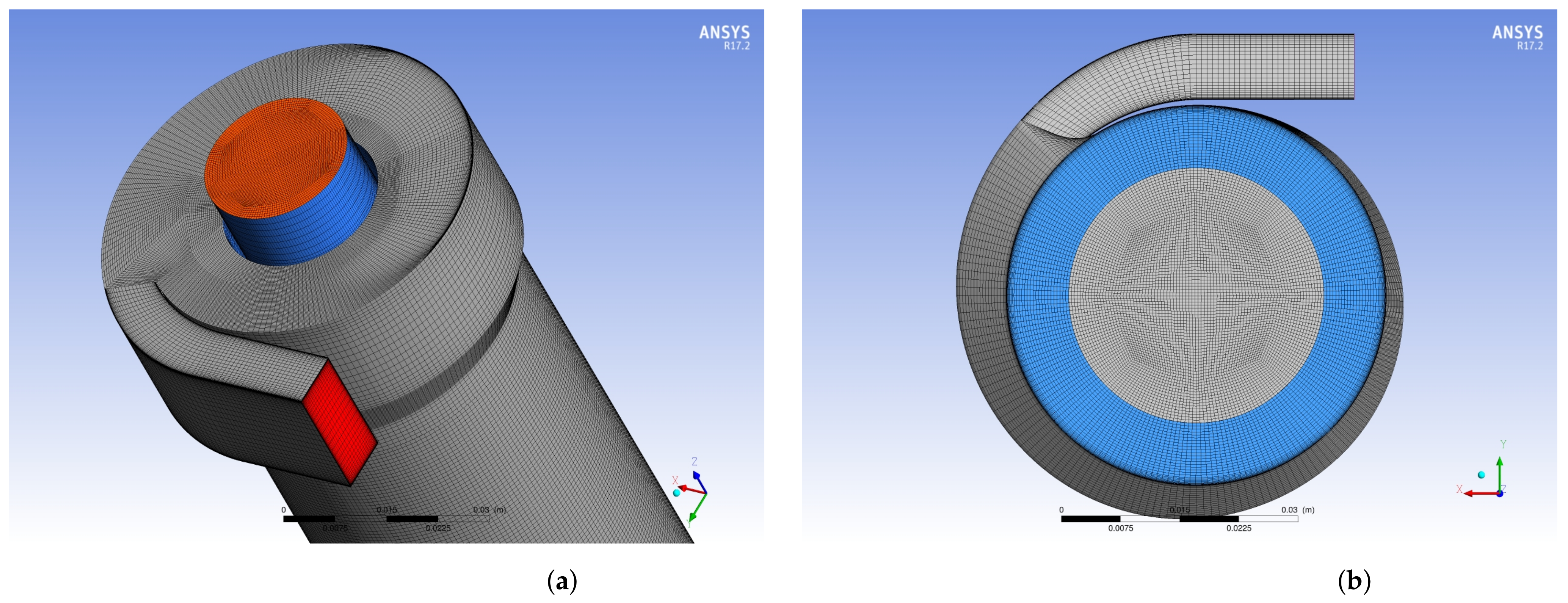
2. Hydrocyclone Geometry and Computational Mesh

The dimensions of the ASH presented in [25] have been used to construct the geometry of the flow domain. The dimensions of the hydrocyclone are shown by Figure 1. The inlet pipe has a rectangular cross-section where its width and depth are (20.32 × 8.38 mm). The cylindrical part of the hydrocyclone has an inner diameter of $48.26$ mm, and its height is 305 mm. There is no conical part for this hydrocyclone. At the bottom, a froth pedestal is placed inside the hydrocyclone to support the air column and froth layer. The pedestal diameter is selected such that the annular exit area equals the area of the overflow pipe ($A_{overflow}/A_{underflow}=1$). The overflow pipe (vortex finder) has an inner diameter of $22.22$ mm and extends a distance of $25.4$ mm (one inch) inside the volute of the hydrocyclone.

To generate a high-quality block-structured grid, the fluid domain was divided into three subdomains, namely the top header, the cylindrical middle part, and exit part that contains the pedestal. The blocks in each subdomain were constructed and grid-generated where the height of the first element normal to wall is nearly 10 microns. The total number of elements of the whole grid is nearly equal to 10.8 million. The grid in the core of hydrocyclone and overflow pipe was designed to resolve the high gradient of tangential and axial velocity components near the region of air core, as shown in Figure 2.

The LES Euler–Euler model in ANSYS-CFX software has been used to simulate the flow of air and water in ASH where water is considered as a continuous phase and air is considered as a dispersed phase. We assumed a uniform spherical air bubble diameter of 500 microns. The motion of the two phases are coupled by modeling the interfacial forces of drag and buoyancy. We use bounded central difference to discretize the continuity and momentum equations of the phases. The bounded central difference schemes are second-order accurate and can damp dispersive errors in central difference schemes. Wang et al. [26] and Xu et al. [27,28] found that the hydrocyclone simulation is not sensitive to the time step between $1.0\times {10}^{-3}$ and $1.0\times {10}^{-4}$, however, we found that a small time step is necessary for the stability and accuracy of the flow velocity components in the ASH. Stable computations are obtained for steps $5\times {10}^{-4}$ and $2.5\times {10}^{-4}$ s. Computations with a larger time step of $1.0\times {10}^{-3}$ s were unstable. The results presented in this paper were obtained with a time step of $5\times {10}^{-4}$ s.

The boundary condition at the inlet was selected as a constant velocity inlet of $v_{inlet}=3.0$ m/s that achieves a mass flow rate of $0.51$ kg/s of water. The water volume fraction at the inlet is 100% (no air). Atmospheric pressure is prescribed at the overflow pipe’s exit boundary, known in CFX as the “opening boundary condition”. This type of boundary condition in CFX allows for reversed air flow to enter the flow domain but without any reversal of the water flow. At the bottom exit annular boundary, pressure is prescribed (also known as pressure outlet boundary condition), and no flow reversal is allowed to enter the flow domain. One of the goals of this paper was to investigate the effects of the prescribed pressure at the underflow boundary on the flow characteristics in ASH. In the actual operation of ASH, the air is injected through a porous tube with a diameter of $48.26$ mm. The designer of ASH [25] recommends an air-to-water flow rate ratio of 3–4. The air-to-water ratio is a parameter that affects the recovery rate of dispersed solid particles. In case flotation kinetics are simulated, the effects of that parameter should also be investigated. The current paper does not include flotation kinetics, and hence the value 4 is used based on a recommendation of the designer of ASH. To avoid modeling airflow in complex network of micro-pores inside the porous pipe, the walls of the hydrocyclone are modeled as no-slip boundaries where zero velocity is prescribed. The air injection was modeled as a mass source of air in a thin annular volume of a radial thickness of $0.33$ mm adjacent to the walls of the hydrocyclone. A mean flux of 47.58 (L/s)/m² was used in the present simulations.

The first simulation is initialized with $100\%$ water with zero velocity in the flow domain and an underflow exit pressure of 6 kPa. Initially, no air is injected. Simulation is continued until an air core is established by air being inhaled by the overflow pipe. The air core took 2 s (4000-time steps) to develop. Then we apply the air mass source and continue the simulation to a statistically steady state. The solution at 6 kPa is used to initialize the simulations for 5 kPa, and so on, for 4 and 3 kPa.

3. Governing Equations for Euler–Euler Model

The two-phase flow of air and water was modeled using the Euler–Euler approach. The motion of the two continuous phases is described by the unsteady filtered Navier–Stokes (LES) equation:

Continuity equation:

$$\frac{\partial \left({\alpha }_i{\rho }_i\right)}{\partial t}+\nabla .\left({\alpha }_i{\rho }_i{\mathbf{V}}_{\mathbf{i}}\right)=S_i$$

(1)

Momentum equation:

$$\frac{\partial \left({\alpha }_i{\rho }_i{\mathbf{V}}_{\mathbf{i}}\right)}{\partial t}+\nabla .\left({\alpha }_i\left({\rho }_i{\mathbf{V}}_{\mathbf{i}}\otimes {\mathbf{V}}_{\mathbf{i}}\right)\right)=-{\alpha }_i\nabla P+\nabla .\left\{{\alpha }_i{\rho }_i\left({\nu }_i+{\nu }_{sgs}\right)\left(\nabla {\mathbf{V}}_{\mathbf{i}}+{\left(\nabla {\mathbf{V}}_{\mathbf{i}}\right)}^T\right)\right\}+{\mathbf{M}}_i+{\alpha }_i{\rho }_i\mathbf{g}$$

(2)

The term ${\mathbf{V}}_i$ denotes the filtered velocity vector of phase i and P denotes the filtered pressure field. The turbulent eddy viscosity term in the above equation is calculated as

$${\nu }_{sgs}=C_m{\Delta }^2\left|\nabla {\mathbf{V}}_{\mathbf{i}}+{\left(\nabla {\mathbf{V}}_{\mathbf{i}}\right)}^T\right|$$

(3)

The $C_m$ is the subgrid model constant. This constant is locally determined in the computational domain using the dynamic model (e.g., Germano et al. [29]). The index (i = 1) denotes the water phase and (i = 2) denotes the air phase. $S_i$ is a mass source of phase i, and ${\mathbf{M}}_i$ is the interfacial force that acts upon phase i due to the presence of other phases. The interfacial momentum exchanges between the two phases accounts for drag and buoyancy on bubbles. The Schiller–Naumann drag model [30] was used to estimate the drag coefficient of the air bubbles. The effects of bubble deformations on the values of the drag coefficient are neglected in the Schiller–Naumann drag model.

4. Validation of Two-Phase Model

The validation of the Euler–Euler LES model by comparison with experimental data is essential to assess the accuracy of the results. Miller et al. [15] conducted experiments using the laser-Doppler anemometer (LDA) without air injection. They measured axial and tangential velocity on a vertical line in a 100 mm hydrocyclone at two different feed rates. However, these experimental velocity measurements in ASH are not suitable for a direct comparison with the CFD results of the present simulations which include air injection. Fayed et al. [10] provided validation for the same computational model for a conventional hydrocyclone. Hsieh and Rajamani [31] and Hsieh [32] conducted experimental measurements in a conventional hydrocyclone using particle image velocimetry (PIV). The profiles of the mean axial and tangential velocity components were reported at different axial locations. Fayed et al. [10] conducted two-phase LES for Hsieh’s hydrocyclone. They studied the effects of grid refinement on the mean velocity profiles and turbulence statistics and showed a good comparison with the experiments. They also studied the effects of the SGS turbulence modeling by comparing the results of the dynamic and Smagorinski models.

5. Results for ASH

The LES two-phase flow model used in the present study was validated by Fayed et al. [10] for a conventional hydrocyclone. They presented grid-independent LES results for the dynamic SGS model, and obtained good agreement with the experimental data for mean flow velocity and turbulence statistics by Hsieh [31]. Therefore, we use the same computational model to simulate the two-phase flow in an air-sparged hydrocyclone. For all the results reported herein, water is considered an incompressible fluid with constant density. We implemented atmospheric pressure at the overflow exit, and uniform velocity was prescribed at the inlet. Different values for static pressure were prescribed at the underflow exit, and their effects on the flow characteristics were investigated.

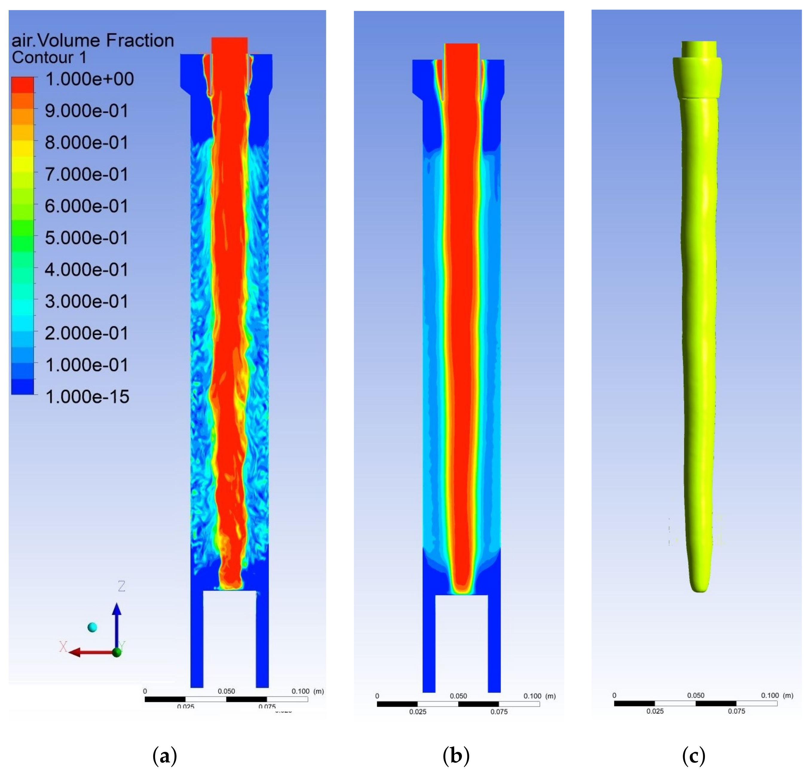
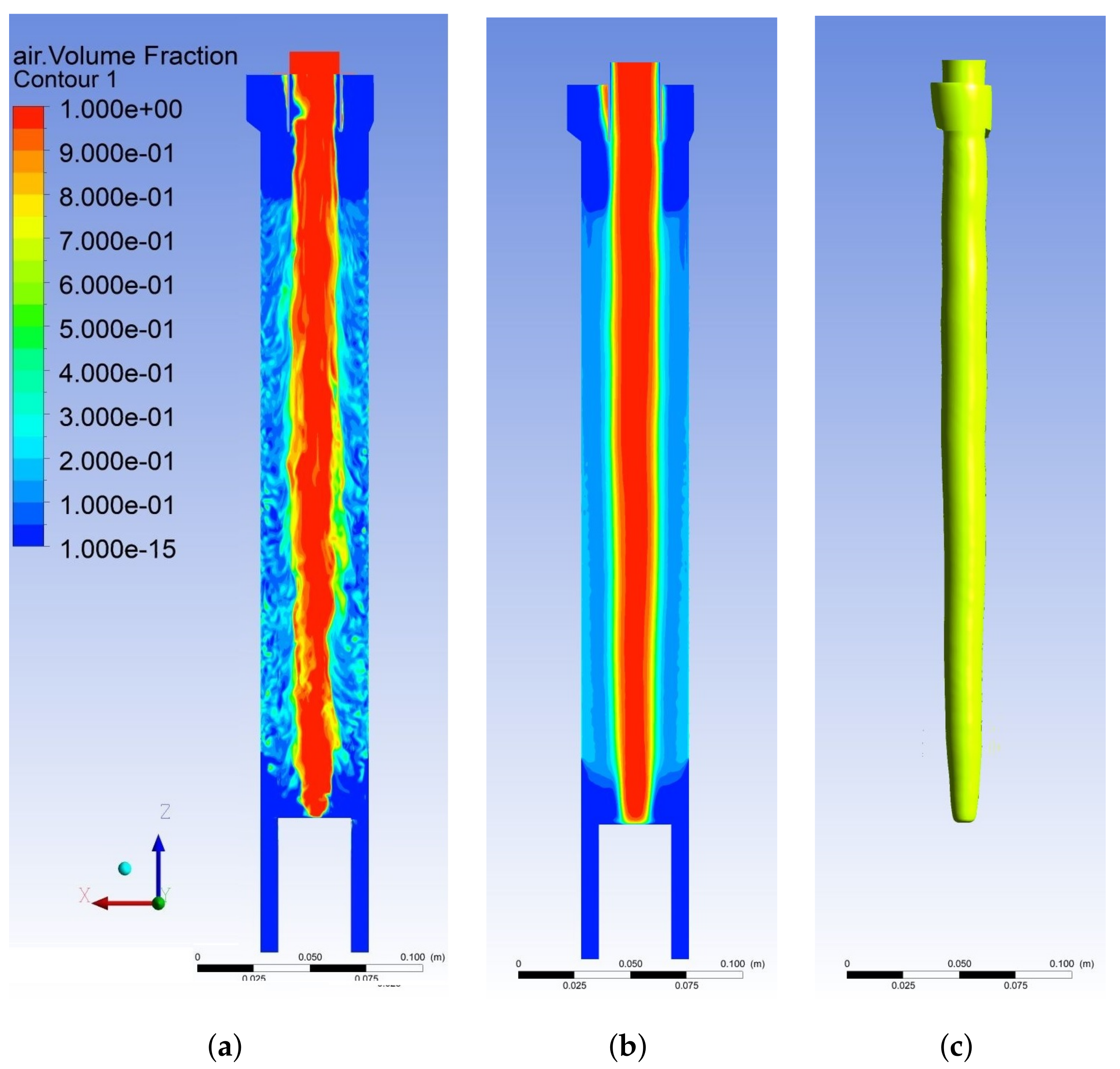
5.1. Air Volume Fraction

The distribution of the air volume fraction in a vertical plane that passes through the axis of ASH is depicted in Figure 3a,b for an exit pressure of 3 kPa. Figure 3a shows a snapshot of the instantaneous air volume fraction (AVF). The air volume fraction is distributed through the swirling layer, where it varies from 0.0% to 100% near the interface of the air core. The contours show that there is no air inside the volute section where the air is injected right below the volute (i.e., the effects of buoyancy are negligible in this type of cyclonic flow). The instantaneous distribution of AVF shows that the pedestal supports the air column and prevents air bubbles from reaching the underflow exit. The contours of instantaneous AVF show a turbulent structure inside the swirling layer in the cylindrical part where the small air bubble of $d_b=0.5$ mm is responsive to the large resolved scales of turbulence in this work. The mean distribution of the air volume fraction was calculated during the course of each simulation, where Figure 3b shows the distribution of mean AVF in a vertical plane that passes through the axis of ASH. The averaging process gives a smoother distribution of AVF and shows a stable air column. Figure 3a,b show that both instantaneous and mean air column extend to and rest on the pedestal. Therefore, the pedestal is essential in the ASH to stabilize the air column and froth layer. The thickness of the water-swirling layer is small at the top part of ASH and increases to reach the maximum value near the pedestal. This distribution of the swirling layer thickness occurs due to the high swirling velocity near the top of the ASH and the lower swirling velocity near the pedestal. This axial distribution of swirling velocity results in a nearly conical air column that is anchored on the pedestal as illustrated by the isosurface of 50% AVF in Figure 3c.

The effects of the underflow pressure on the structure of the air column in ASH were studied. Figure 4a shows the instantaneous distribution of air volume fraction in a vertical plane that passes through the axis of the ASH for an underflow exit pressure of 4 kPa. The distribution of AVF shows that the radial thickness of the water swirling layer is larger than that for the previous case, where the exit underflow pressure was equal to 3kPa. Figure 4b shows the distribution of the mean AVF in the air column for an exit underflow pressure of 4 kPa where it anchors on the pedestal. The local mean diameter of the air column is smaller than that of the exit underflow pressure of 3 kPa. This observation is illustrated by comparing the air column shown by Figure 3c and Figure 4c. The distribution of AVF at a higher exit underflow flow pressure of 5 kPa is shown by Figure 5a–c for instantaneous and mean values. The underflow pressure increases the radial thickness of the water swirling layer, where the thickness becomes nearly uniform in the axial direction. The mean distribution of AVF and air column for this value of underflow pressure are shown by Figure 5b,c. The average diameter of the air column is nearly equal to the diameter of the overflow pipe, as shown by Figure 5b. The mean distribution shows that the structure of the air column has an upside-down conical shape for an underflow pressure of 3 kPa, 4 kPa, and 5 kPa exit pressure at the underflow, as shown by Figure 3c, Figure 4c and Figure 5c. The distributions of AVF are presented for an underflow pressure of 6 kPa, as depicted by Figure 6a–c. The radial thickness of the water-swirling layers is larger than those for underflow pressure values of less than 6 kPa. The structure of the air column is cylindrical, and its diameter is lower than the diameter of the overflow pipe, as shown by Figure 6b. The diameter of the air core decreases as we increase the pressure at the underflow exit section. In other words, the thickness of the water swirling layer increases with the increasing underflow pressure, and hence the performance of ASH can be controlled by controlling the pressure at the underflow section.

To investigate the thickness of the swirling layer, the profiles of the mean water volume fraction (WVF) are plotted at different axial locations. We consider the water swirling layer to end at the mean water volume fraction of 50%. The vertical (axial) locations $z1$, $z2$, $z3$, and $z4$ of each profile are measured from the top roof of the ASH ($z=0$). The values of $z1$, $z2$, $z3$, and $z4$ are −50, −150, −250, and −300 mm, respectively. Air is injected in a cylindrical shell of a vertical extent of 250 mm that extends from $z=-50$ mm to $z=-300$ mm. The profiles of the mean WVF show the radial variations of the swirling layer thickness as we move down through the cylindrical part of ASH. As shown by Figure 7a–d, the radial thicknesses of the swirling layer at z1, z2, z3, and z4 are nearly equal to 2.6 mm, 7.5 mm, 12 mm, 14 mm, respectively, for exit underflow pressure values of 3 kPa. It is obvious from these values that the radial thickness of the swirling water layer is increasing nearly linearly as we move downward and reaches its maximum at the pedestal. These mean values of the radial thickness of the water swirling layer versus the axial distances are presented in

Table 1. Thickness of the water swirling layer at different axial distances of z1, z2, z3, and z4 and underflow exit pressure values. Radius of ASH $R=24.13$ mm.

Under-Flow Pressure (kPa)	3	4	5	6
$\Delta$$r_1\left(z_1\right)$	2.64	8.09	13.13	13.92
$\Delta$$r_2\left(z_2\right)$	7.52	11.68	12.95	13.33
$\Delta$$r_3\left(z_3\right)$	12.05	13.38	14.01	14.31
$\Delta$$r_4\left(z_4\right)$	14.05	14.77	15.46	15.79

. This table shows the strong dependence of the radial thickness distribution of the swirling layer on the value of pressure at the underflow section. Therefore, the designer of the ASH can control its performance by changing the pressure at the underflow exit that changes the residence time and split ratio of water to achieve optimal operating conditions.

The split ratio was monitored over the course of the simulation and averaged over time. It is calculated as the percentage of the inlet water mass flow rate that flows through the overflow pipe. The values of the water mass flow rate at the overflow exit were monitored with time for each value of the underflow pressure. The split ratio for an exit pressure of $P_2=$ 3 kPa is low and approximately 5.7% of the inlet flow mass rate, as given in

Table 2. Water Split Ratio.

${\mathit{P}}_2$ kPa	Split Ratio
3	5.71
4	8.96
5	15.9
6	26.0

. The split ratio increases as we increase the value of the exit underflow pressure. For an exit pressure of $P_2=$ 4 kPa, the average split ratio is approximately 9%. The split ratio for $P_2=$ 5 kPa is approximately 16%. At $P_2=$ 6 kPa, the split ratio reaches 26% of the inlet flow rate. The dependence of the split ratio on the exit pressure at the underflow is due to the change in the radial thickness of the swirling layer as described above.

5.2. Mean Velocity Field

Figure 8 shows the contours for the axial and swirling (tangential) components of water superficial velocity for an underflow exit pressure of 5 kPa. The figure identifies regions of high velocities within the swirling layer and its variation with axial distance from the roof of the hydrocyclone. Figure 8a shows the radial distribution of the mean water superficial axial velocity where the flow near the wall is downward and upward near the interface of the air column. Figure 8b describes the mean tangential water velocity contours for the underflow exit pressure of 5 kPa. The maximum tangential velocity prevails in the volute section. The superficial tangential water velocity in the air core is almost zero. As the flow swirls downward, the tangential velocity decreases while the thickness of the swirling layer increases.

The thickness of the swirling water layer and the shape of the air column depend on the swirling velocity and the axial downward velocity. The swirling velocity is determined by the feed rate at the inlet section, while the axial velocity distribution depends on the value of underflow exit pressure. For a better understanding of ASH performance, we investigate the radial distribution of the water superficial axial and tangential velocity complements at different axial locations. In the above section, we observed that low values of exit pressure create a thin swirling layer. Herein, we investigate the profiles of the water’s superficial axial and tangential velocity for different values of exit pressure. The mean water superficial axial velocity profiles at different vertical locations of $z1$, $z2$, $z3$, and $z4$ are depicted in Figure 9a for an exit pressure $P_2=3$ kPa. At $z1$, the water’s superficial axial velocity has a maximum downward value of $-1.5$ m/s at $r=22$ mm and the profile shows rapid change in the radial direction and high shear near the wall. The profile shows zero axial velocity (ZAV) at r = 20.5 mm. For $0<r<20.5$ mm, the water’s superficial axial velocity remains very small and has positive values (i.e., upward). At the $z2$ location, the maximum downward water superficial axial velocity reaches −0.7 m/s and ZAV at r = 16 mm. The profile at this location shows a central region where the water’s superficial axial velocity is positive (upward) for the $0<r<16$ mm range. As we move further downward, the profiles show smoother radial variation, and a maximum downward water superficial axial velocity decreases to −0.55 m/s at $z3$ and −0.45 m/s at $z4$. The profiles of the water’s superficial axial velocity and the above profiles for WVF show that the axial velocity becomes high in the region of the thin swirling layer. The thickness of the swirling layer increases as we move downward while the axial velocity decreases in magnitude.

Next, we investigate the velocity profiles for an underflow exit pressure of $P_2$ = 4, 5, and 6 kPa. Axial and tangential velocity components and the air/water volume fraction were averaged over time. The profiles of the mean water superficial axial velocity are shown by Figure 9b–d, respectively. The mean axial velocity profiles show an asymmetric distribution of the axial velocity. The asymmetry occurs because of the flow feed through one volute. The axial velocity profiles for $P_2=3$ kPa are similar in shape to the profile at $P_2$ = 4 kPa. The profiles at $z2$ show a maximum downward velocity of nearly −0.65 m/s. The axial velocity changes in the radial direction and reaches zero at different radial locations. Then, the profiles show positive upward velocity distribution. The magnitude of upward velocity increases with the increasing exit pressure. The profiles flatten as we move downward due to the increased thickness of the swirling layer. The locations of zero axial velocity change with exit pressure and vertical location.

It is important to note that the stability of the air column and froth layer is determined by the radial distribution of the water tangential velocity. The flow in ASH looks like a column vortex of water with an air core. The profiles of the water superficial tangential velocity at three vertical locations are shown in Figure 10 for different values of the exit pressure at the underflow exit. The profiles show that the flow in the boundary layer is resolved. The swirling layer’s thickness depends on the exit pressure value $P_2$ as presented above. At the top part of ASH, $z2=-150$ mm, the swirling water layer is thin for $P_2=$ 3 kPa but then increases as the exit pressure increases to $P_2=6$ kPa. The profiles exhibit a high gradient because of the thin swirling layer. This increase in the thickness of the swirling layer near the top region of ASH is widening the radial distribution of the water tangential velocity. As the exit pressure increases, the maximum value of the tangential velocity increases from 2 m/s at $P_2=$ 3 kPa to 2.3 m/s at $P_2=$ 6 kPa. The profiles at different vertical locations $z3=-250$ mm and $z4=-300$ mm show similar behavior.

The pressure imposed at the underflow exit controls the distribution of flow velocities inside the ASH. If the exit pressure equals zero (gauge pressure), the swirling layer becomes very thin through the whole cylindrical part of ASH. Therefore, the exit pressure is a crucial parameter for controlling the thickness of the swirling layer and the distribution of the water’s superficial axial and tangential velocities.

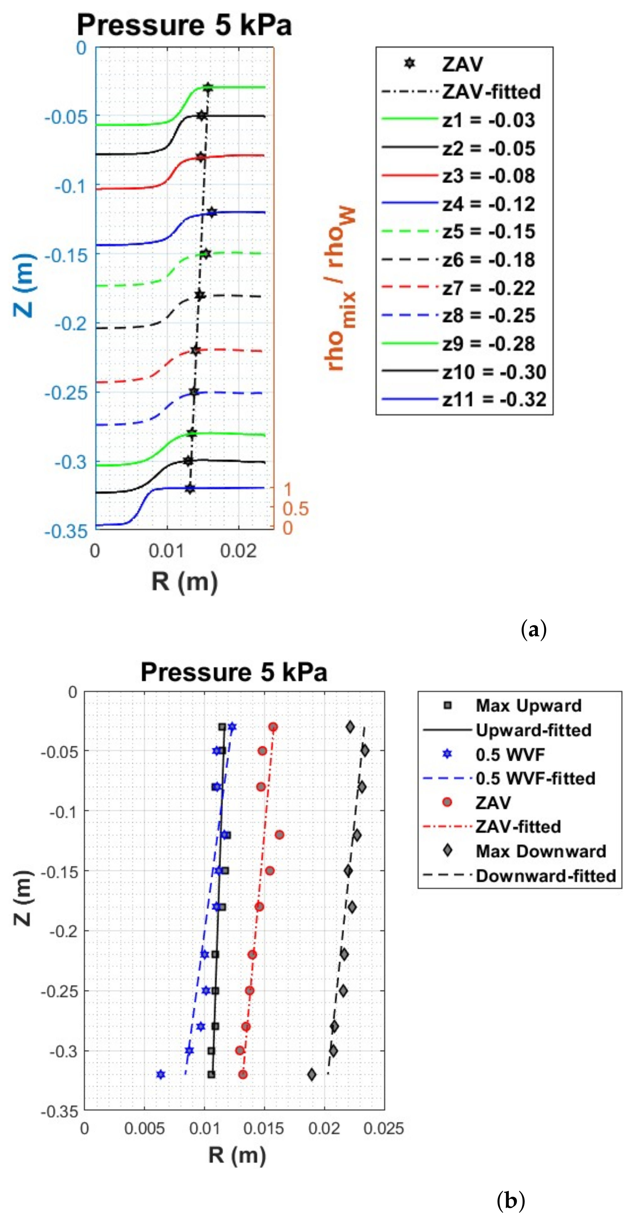
5.3. Zero Axial Velocity (ZAV) and Mixture Density

The above profiles show that axial velocity in ASH is negative (downward) near the wall and upward (positive) near the air core. Miller et al. [25] measured the vertical distribution of the zero axial velocity (ZAV) locations using computer tomography (CT) scanning. They investigated the effects of the ratio of air/slurry and the overflow/underflow area ratio on the location of the ZAV. Miller et al. [25] reported the ZAV surface for an overflow/underflow area ratio of 0.74 based on a CFD model. They observed in their experiments and CFD simulations that the location of the ZAV surface is critical for the split ratio of the overflow. Our LES model of two-phase flow in ASH predicts the location of the ZAV surface. The following section presents a discussion of the loci of ZAV and the distribution of mixture density in ASH.

The isosurface of the zero axial velocity (ZAV) inside ASH separates an upward water flow and downward water flow. The net upward flow goes to the overflow, and the net downward flow exits through the underflow section. The location of the ZAV’s surface is influenced by the inlet feed rate and the underflow exit pressure. Our LES simulations predict the loci of the ZAV versus the vertical coordinate. Furthermore, we show the loci of ZAV relative to the profiles of mixture density. The local mixture density is computed as

$${\rho }_m={\alpha }_{air}{\rho }_{air}+{\alpha }_{water}{\rho }_{water}$$

(4)

where ${\alpha }_{air}$ and ${\alpha }_{water}$ denote the local volume fractions of air and water, respectively. The radial profiles of the mixture density at different vertical locations are presented in Figure 11a. The radial locations of zero axial velocity were determined for each axial velocity profile. Figure 11a shows the profiles of the mixture density and their intersection with the ZAV line at an exit pressure of 3 kPa. The ZAV line intersects with the profiles of mixture density in the air column in the range of $z<\left|-120\right|$ mm, where the mixture density is nearly equal to the air density. The vertical distance is measured from the top roof of the hydrocyclone. For $z>\left|-120\right|$ mm, the intersection of the ZAV line with radial density profiles occurs inside the swirling layer where the density of the mixture is nearly equal to that of water density. We recall that the flow inside the ZAV isosurface is upward and that between the ZAV isosurface and hydrocyclone wall is downward. The ASH has most of the water flow going downward in the top region of $z<\left|-120\right|$ mm for exit pressure 3000 Pa. The intersection of the ZAV line with the mixture density profiles indicates that the flow of water is recirculating downward in the region $z<\left|-120\right|$ mm and this flow behavior reduces the overflow split ratio.

Because of the turbulent fluctuations, the instantaneous location of the ZAV line is changing, and the flow rate of water through the overflow changes with time. The average locations of ZAV, the maximum upward and downward water superficial axial velocity versus the vertical coordinate z are shown in Figure 11b. This figure depicts the average loci of 50% water volume fraction (blue curve). The loci of maximum positive upward axial velocity (solid black line) is located on the left of the ZAV line (red line). In contrast, the loci of the maximum negative downward axial velocity (dashed black line) are located on the right (i.e., inside the swirling layer). The line representing 50% of the water volume fraction (blue line) intersects with the ZAV line (red line) at a $z\approx -120$ mm. This intersection of the ZAV line with the mixture density profile separates the water flowing down from that flowing upward. In the region $z>-120$ mm, the water flows downward, and for $z>-120$ mm, a percentage of the water flows upward to the overflow exit.

The loci of zero axial velocity (ZAV) for $P_2=$ 4 kPa were computed for each axial velocity profile as a function of the radius. Figure 12a shows the profiles of the radial distribution of the mixture density and the intersection with the ZAV line. The ZAV line intersects with the radial mixture profiles at the boundary of the air column where the mixture density is nearly equal to 0.5 ${\rho }_{water}$ in the range of $z<-50$ mm. The air injection starts at $z=-50$ mm and ends at $z=-300$ mm. Most water flow goes downward in the top region $z>-50$ mm. The intersection of the ZAV line indicates that the downward flow of water is less than that for an exit pressure of 3 kPa, and the overflow split ratio increases to nearly 7.0%. The average radial locations of ZAV as well as the maximum upward and downward water superficial axial velocities versus the vertical axis z are shown in Figure 12b. The average loci of 50% water volume fraction (blue curve) are also shown in this figure. The loci of the maximum positive upward axial velocity (solid black line) is located on the left of the ZAV line (red line). In contrast, the loci of the maximum negative downward axial velocity (dashed black line) are located on the left (i.e., inside the swirling layer). The line representing 50% water volume fraction (blue line) intersects with the ZAV line (red line) at a $z\approx -50$ mm.

The loci of the zero axial velocity for $P_2=$ 5 kPa and $P_2=$ 6 kPa were determined for each axial velocity profile as a function of the radius. Figure 13a and Figure 14a show the profiles of radial distribution of the mixture density and the intersection of ZAV lines with these profiles for exit pressures of 5 kPa and 6 kPa. The ZAV line intersects with the radial mixture profiles in the swirling layer where the mixture density is nearly equal to that of water density ${\rho }_{water}$ in the whole domain. The intersection of the ZAV line occurs right at the bottom section of the volute. The intersection of the ZAV line with profiles of mixture density indicates that the upward flow of water is higher for exit pressures of 5 kPa and 6 kPa than those of 3 and 4 kPa. The overflow split ratio is nearly 16% and 26.12% for $P_2=$ 5 kPa and $P_2=$ 6 kPa, respectively. The average radial locations of ZAV as well as the maximum upward and downward water superficial axial velocities versus the vertical axis z are shown in Figure 13b and Figure 14b. The average loci of 50% water volume fraction (blue curve) are also shown in this figure. The loci of the maximum positive upward axial velocity (solid black line) is located on the left of the ZAV line (red line). In contrast, the loci of the maximum negative downward axial velocity (dashed black line) are located on the left (i.e., inside the swirling layer). The line representing 50% water volume fraction (blue line) is located on the left side of the ZAV line, and no intersection occurs.

5.4. Flow Angle

The flow angle is another parameter representing the flow direction inside the swirling layer. The flow angle is calculated according to the following equation

$$\beta =ta{n}^{-1}\left(\frac{v_{wa}}{v_{wt}}\right)$$

(5)

where $v_{wa}$ and $v_{wt}$ denote the water superficial axial and tangential velocity components, respectively, and the profiles of flow angle in degrees at different values of exit pressure and different axial locations are shown in Figure 15. The angle is negative for downward flow near the wall, but it changes sign at the ZAV surface and becomes positive in the upward-moving water. The underflow exit pressure affects the thickness of the swirling layer and the distribution of the water tangential and axial velocity. As a result, the distribution of flow angles in the radial direction is accordingly affected by the values of an exit pressure of $P_2$. At $z=-150$ mm, the flow angle is approximately −20° near the wall. Figure 15a shows that the values of flow angles are nearly zero at the radius of $r\approx 15$ mm. For $r<15$ mm, the flow angles have positive values. Therefore, the flow goes downward between the wall and a radius of 15 mm and upward in the center of the cyclone between radii of 15 and zero mm. At $z3=-250$ mm, the flow angle is also nearly −20° in the neighborhood of walls and increases to a value of zero at the radius $r=13$ mm, as shown in Figure 15b. The flow takes a longer distance to change its direction from 20° to zero degrees at $z3=-250$ mm, which indicates a thicker swirling layer as the flow goes downwards. The water volume fraction is very small at the center $r=0$, and a flow angle based on water superficial velocity may be considered an approximate air–water mixture. The flow between $r=13$ and $r=-13$ mm goes upward more sharply than at $z2=-150$ mm. At the bottom section, $z4=-300$ mm, Figure 15c shows that the flow angle is nearly 20° near the wall and reaches zero value at $r\approx 12.5$ mm. However, the flow in the center between $r=12.5$ and $r=-12.5$ mm has a unique behavior that shows a reduction in the direction of upward flow from approximately 10° to 5° between $r\approx 10$ mm and $r\approx 6.5$ mm. The upward flow is squeezed in the small area with a diameter of approximately 13 mm and a sharper gradient. The ZAV is located at a flow angle of zero degrees. We deduce from these figures that maximum negative flow angles occur near the wall region.

Table 3. Radii of the air column at different vertical locations in mm.

Under-Flow Pressure (kPa)	3	4	5	6
$r_1$, $z_1$	21.49	16.04	11.00	10.21
$r_2$, $z_2$	16.61	12.45	11.18	10.8
$r_3$, $z_3$	12.08	10.75	10.12	9.82
$r_4$, $z_4$	10.08	9.36	8.67	8.34

gives the radial boundaries of the air columns. We observe that the flow angles vary from $+20$ at the boundaries of the air core to $+90$ near the center line of ASH, where the flow is 100% upward.

5.5. Turbulent Kinetic Energy

The water turbulent kinetic energy distribution at the pressure of 5 kPa is shown in Figure 16. Significant turbulence production is found in the volute section, but once the flow swirls down the cylindrical section, the high turbulent kinetic energy is confined in a thin layer near the wall. The thickness of that layer increases as the flow reaches the pedestal. Figure 16b also shows the water turbulence kinetic energy on various horizontal planes. The first three horizontal planes at the top have immense turbulent kinetic energy, and their magnitudes decrease for the following seven horizontal planes. For the last three planes, the magnitude of the water turbulence kinetic energy increases near the froth pedestal. Figure 16c shows isosurfaces for the water tangential vorticity fluctuation (${\omega }_{\theta }^{\prime }=\pm 200$ s⁻¹) that indicate vortex filaments of opposite rotations elongated in the circumferential direction.

5.6. Instantaneous Velocity and Energy Spectra

The velocity components are recorded in time at four test points, as shown in Figure 16a. The coordinates of the points are:

$$(x,y,z)=(0.013,0,-0.08),(0.0239,0,-0.08),(0.0239,0,-0.208),(0.014,0,-0.253),$$

respectively, where $x,y,$ and $z$ are in meters. Figure 17a depicts the time history of water velocity components at point p1, which is located just below the inlet of the hydrocyclone and at the interface between the air core and swirling water layer. The axial and radial velocities are of the same order and appear to have mean values of zero. The tangential velocity component has a significantly larger mean value of approximately $1.1$ m/s. Time history indicates that the turbulence reached a steady state. Point p2 is at the same elevation as point p1 but very close to the wall. The axial and tangential velocities at this location show large fluctuations, but the radial velocity is small both in mean and fluctuations. At point p3, near the wall, the dominant velocity components are the tangential and axial velocities. The radial velocity component is of a much smaller mean and fluctuating magnitude. Point p4 is near the interface between the air core and the swirling water layer. Here, at point p4, the radial and axial velocities are of the same order, but the tangential velocity is significantly larger. The stronger fluctuations imply a significant increase in the turbulent kinetic energy near the bottom of the hydrocyclone. The velocity–time signals at points p2 and p3 show strong velocity fluctuations in the tangential and axial velocities near the wall. This explains the high levels of turbulent kinetic energy evident in Figure 16a.

The one-dimensional energy spectra corresponding to the time signals of Figure 17 are computed by Welch’s method [33] and presented in Figure 18. There is a striking difference between the spectra for near-wall points (p2 and p3) and points near the air core boundary (p1 and p4). For the near-wall points, the turbulent energy of small scales decays as $f^{-4}$, and no significant inertial subrange is visible. The axial and tangential velocity fluctuations are two orders of magnitude greater than the radial component. Hence, the turbulence appears to be two-dimensional near the wall. Various theoretical studies and numerical simulations of two-dimensional turbulence predict that energy spectra at small scales of the form $k^{-n}$, where n is 3 or 4, and k is the wavenumber. Such power laws are due to an enstrophy cascade (e.g., Lesieur [34]). In particular, Saffman [35] studied the decay of two-dimensional turbulence and predicted an energy spectrum of $k^{-4}$. Herring et al. [36] also conducted direct numerical simulations of decaying two-dimensional turbulence and found a law of $k^{-4}$. Fayed et al. [10] also predicted the $f^{-4}$ power law for the near-wall turbulence of a conventional hydrocyclone. For points on the air core boundary, a short inertial subrange of slope −5/3 is found, followed by the viscous dissipation of the small scales with a slope of −7 or −8. For the near-wall points, the main contributors to the turbulent energy are the tangential and axial velocity fluctuations, while the contribution of the radial velocity is much smaller. Thus, the small-scale turbulence is highly anisotropic. The spectra for the axial and radial velocity components are nearly identical for the points at the air–water interface. Qualitative differences in the turbulence characteristics from one region to another in a hydrocyclone make it difficult to produce meaningful results using a Reynolds-averaged Navier–Stokes solver with simple turbulence models such as eddy viscosity models.

5.7. Conclusions

We conducted large-eddy simulations for a two-phase flow of air and water in an air-sparged hydrocyclone (ASH) using the Euler–Euler (two-fluid) approach. Air bubbles of a uniform diameter of $0.5$ mm are assumed for the gas phase. An eddy viscosity subgrid-scale model is used, and a dynamic model is used to compute the model coefficient. The governing equations were discretized and solved on a hexahedral O-type grid with 10.5 million elements. The LES model was validated by Fayed et al. [10] for a two-phase flow in a conventional hydrocyclone using experimental data by Hsieh [31]. The LES results of ASH show the dependence of the swirling layer thickness and axial and tangential velocity distribution on the pressure imposed at the underflow exit. Miller et al. [25] recommended that the ZAV line coincides with the air column and froth layer. In this study, the loci of the zero axial velocity (ZAV) of water were analyzed, and their implications for the split ratio were highlighted. The split ratios of approximately 6%, 9%, 16%, and 26% were obtained at exit pressures of $P_2=$ 3, 4, 5, and 6 kPa, respectively. The CFD results of ASH show that the value of the exit pressure should be in the range of $3<P_2<4$ kPa to obtain a split ratio which is less than 16%. The turbulent energy spectra indicate a $f^{-4}$ law for near-wall points, where f is frequency, and an inertial subrange of $f^{-5/3}$ for points at the air–water interface.

References

1. Vakamalla, T.R.; Mangadoddy, N. Comprehensive dense slurry CFD model for performance evaluation of industrial hydrocyclones. Ind. Eng. Chem. Res. 2021, 60, 12403–12418. [Google Scholar] [CrossRef]
2. Tailleur, R.G.; Peretti, A.G. Hydrocyclone settler (HCS) with internal hydrogen injection: Measure of internal circulation and separation efficiencies of a three-phase flow. Ind. Eng. Chem. Res. 2020, 59, 1261–1276. [Google Scholar] [CrossRef]
3. Svarovsky, L. Hydrocyclones; Holt, Rinehart and Winston Ltd.: Austin, TX, USA, 1984. [Google Scholar]
4. Wills, B.A.; Finch, J.A. Wills’ Mineral Processing Technology: An Introduction to the Practical Aspects of Ore Treatment and Mineral Recovery; Butterworth-Heinemann: Portsmouth, NH, USA, 2015. [Google Scholar]
5. Bretney, E. Water Purifier. US Patent No. 453105, 26 May 1891. [Google Scholar]
6. Banerjee, C.; Chaudhury, K.; Majumder, A.K.; Chakraborty, S. Swirling flow hydrodynamics in hydrocyclone. Ind. Eng. Chem. Res. 2015, 54, 522–528. [Google Scholar] [CrossRef]
7. Chu, L.Y.; Luo, Q.; Yu, R.H. Concentration and classification characteristics in a modified air-sparged hydrocyclone (ASH). Int. J. Miner. Process. 1996, 48, 73–93. [Google Scholar] [CrossRef]
8. Gonçalves, S.M.; Kyriakidis, Y.N.; Ullmann, G.; Barrozo, M.A.d.S.; Vieira, L.G.M. Design of an optimized hydrocyclone for high efficiency and low energy consumption. Ind. Eng. Chem. Res. 2020, 59, 16437–16449. [Google Scholar] [CrossRef]
9. Ghodrat, M.; Kuang, S.B.; Yu, A.B.; Vince, A.; Barnett, G.D.; Barnett, P.J. Computational study of the multiphase flow and performance of hydrocyclones: Effects of cyclone size and spigot diameter. Ind. Eng. Chem. Res. 2013, 52, 16019–16031. [Google Scholar] [CrossRef]
10. Fayed, H.; Bukhari, M.; Ragab, S.A. Large-eddy simulation of a hydrocyclone with an air core using two-fluid and volume-of-fluid models. Fluids 2021, 6, 364. [Google Scholar] [CrossRef]
11. Monredon, T.C.; Hsieh, K.T.; Rajamani, R.K. Fluid flow model of the hydrocyclone: An investigation of device dimensions. Int. J. Miner. Process. 1992, 35, 65–83. [Google Scholar] [CrossRef]
12. Hararah, M.A.; Endres, E.; Dueck, J.; Minkov, L.; Neesse, T. Flow conditions in the air core of the hydrocyclone. Miner. Eng. 2010, 23, 295–300. [Google Scholar] [CrossRef]
13. Slack, M.D.; Del Porte, S.; Engelman, M.S. Designing automated computational fluid dynamics modelling tools for hydrocyclone design. Miner. Eng. 2004, 17, 705–711. [Google Scholar] [CrossRef]
14. Lelinski, D.; Bokotko, R.; Hupka, J.; Miller, J.D. Bubble generation in swirl flow during air-sparged hydrocyclone flotation. Min. Metall. Explor. 1996, 13, 87–92. [Google Scholar] [CrossRef]
15. Miller, J.D.; Upadrashta, K.R.; Kinneberg, D.J.; Gopalakrishnan, S. Fluid-flow phenomena in the air-sparged hydrocyclone. In Proceedings of the XVth International Minerals Processing Congress, Cannes, France, 2–9 June 1985; pp. 87–99. [Google Scholar]
16. Miller, J.D. The Concept of an air-sparged hydrocyclone. In Proceedings of the 110 THAIM E Annual Meeting, Chicago, IL, USA, 22–26 February 1981; pp. 1–10. [Google Scholar]
17. Miller, J.D. Air-Sparged Hydrocyclone and Method. US Patent No. 4279743, 21 July 1981. [Google Scholar]
18. Van Camp, M.C. Development of the Air Sparged Hydrocyclone for Flotation in a Centrifugal Field. Ph.D. Thesis, Department of Metallurgy and Metallurgical Engineering, University of Utah, Salt Lake City, UT, USA, 1981. [Google Scholar]
19. Yalamanchili, M.R.; Miller, J.D. Removal of insoluble slimes from potash ore by air-sparged hydrocyclone flotation. Miner. Eng. 1995, 8, 169–177. [Google Scholar] [CrossRef]
20. Miller, J.D.; YE, Y. Froth characteristics in air-sparged hydrocyclone flotation. Miner. Process. Extr. Metall. Rev. 1989, 5, 307–327. [Google Scholar] [CrossRef]
21. Miller, J.D.; Das, A. Swirl flow characteristics and froth phase features in air-sparged hydrocyclone flotation as revealed by X-ray CT analysis. Int. J. Miner. Process. 1996, 47, 251–274. [Google Scholar]
22. Gopalakrishnan, S. Development of the Air-Sparged Hydrocyclone for Froth Flotation in a Centrifugal Field. Ph.D. Thesis, The University of Utah, Salt Lake City, UT, USA, 1991. [Google Scholar]
23. Van Deventer, J.; Burger, A.; Cloete, F. Intensification of flotation with an air-sparged hydrocyclone. J. S. Afr. Inst. Min. Metall. 1988, 88, 325–332. [Google Scholar]
24. Baker, M.W.; Gopalakrishnan, S.; Rogovin, Z.; Miller, J.D. Hold-up volume and mean residence time measurements in the air-sparged hydrocyclone. Part. Sci. Technol. 1987, 5, 409–420. [Google Scholar] [CrossRef]
25. Miller, J.D.; Das, A. Flow phenomena and its impact on air-sparged hydrocyclone flotation of quartz. Min. Metall. Explor. 1995, 12, 51–63. [Google Scholar] [CrossRef]
26. Wang, B.; Chu, K.W.; Yu, A.B. Numerical study of particle- fluid flow in a hydrocyclone. Ind. Eng. Chem. Res. 2007, 46, 4695–4705. [Google Scholar] [CrossRef]
27. Xu, Y.; Song, X.; Sun, Z.; Lu, G.; Li, P.; Yu, J. Simulation analysis of multiphase flow and performance of hydrocyclones at different atmospheric pressures. Ind. Eng. Chem. Res. 2012, 51, 443–453. [Google Scholar] [CrossRef]
28. Xu, Y.; Song, X.; Sun, Z.; Tang, B.; Li, P.; Yu, J. Numerical investigation of the effect of the ratio of the vortex-finder diameter to the spigot diameter on the steady state of the air core in a hydrocyclone. Ind. Eng. Chem. Res. 2013, 52, 5470–5478. [Google Scholar] [CrossRef]
29. Germano, M.; Piomelli, U.; Moin, P.; Cabot, W.H. A dynamic subgrid-scale eddy viscosity model. Phys. Fluids A 1991, 3, 1760–1765. [Google Scholar] [CrossRef]
30. Clift, R.; Grace, J.R.; Weber, M.E. Bubbles, Drops and Particles; Dover Publications: Mineola, NY, USA, 2005. [Google Scholar]
31. Hsieh, K.T.; Rajamani, K. Phenomenological Model of The Hydrocyclone: Model Development and Verification for Single-Phase Flow. Int. J. Miner. Process. 1988, 22, 223–237. [Google Scholar] [CrossRef]
32. Hsieh, K.T. Phenomenological Model of the Hydrocyclone. Ph.D. Thesis, University of Utah, Salt Lake City, UT, USA, 1988. [Google Scholar]
33. Welch, P. The use of fast Fourier transform for the estimation of power spectra: A method based on time averaging over short, modified periodograms. IEEE Trans. Audio Electroacoust. 1967, 15, 70–73. [Google Scholar] [CrossRef]
34. Lesieur, M. Turbulence in Fluids; Springer: Dordrecht, The Netherlands, 2008. [Google Scholar]
35. Saffman, P.G. On the spectrum and decay of random two-dimensional vorticity distributions at large Reynolds number. Stud. Appl. Math. 1971, 50, 377–383. [Google Scholar] [CrossRef]
36. Herring, J.R.; Orszag, S.A.; Kraichnan, R.H.; Fox, D.G. Decay of two-dimensional homogeneous turbulence. J. Fluid Mech. 1974, 66, 417–444. [Google Scholar] [CrossRef]
Figure 1. Dimensions of Miller’s 2-inch ASH [25].
Fluids 08 00139 g001
Figure 2. Computational grid of 2-inch ASH. (a) surface mesh; and (b) mesh on a volute section.
Fluids 08 00139 g002
Figure 3. Air volume fraction for an exit pressure of 3 kPa. (a) Instantaneous air volume fraction; (b) Mean air volume fraction; and (c) Isosurface of 50% air volume fraction.
Fluids 08 00139 g003
Figure 4. Air volume fraction for the exit pressure of 4 kPa: (a) Instantaneous air volume fraction; (b) mean air volume fraction; (c) isosurface of 50% air volume fraction.
Fluids 08 00139 g004
Figure 5. Air volume fraction for an exit pressure of 5 kPa: (a) instantaneous air volume fraction; (b) mean air volume fraction; and (c) isosurface of 50% air volume fraction.
Fluids 08 00139 g005
Figure 6. Air volume fraction for exit pressure of 6 kPa; (a) instantaneous air volume fraction; (b) mean air volume fraction; and (c) isosurface of 50% air volume fraction.
Fluids 08 00139 g006
Figure 7. Effect of the underflow exit pressure on the profiles of the mean water volume fraction at different axial locations: (a) 3 kPa exit pressure; (b) 4 kPa exit pressure; (c) 5 kPa exit pressure; and (d) 6 kPa exit pressure.
Fluids 08 00139 g007
Figure 8. Axial and tangential water velocity contours for pressure 5 kPa: (a) mean axial water velocity; and (b) mean tangential water velocity.
Fluids 08 00139 g008
Figure 9. Profiles of mean water superficial axial velocity at different axial locations: (a) 3 kPa exit pressure; (b) 4 kPa exit pressure; (c) 5 kPa exit pressure; and (d) 6 kPa exit pressure.
Fluids 08 00139 g009
Figure 10. Profiles of water superficial tangential velocity at z2, z3, and z4: (a) WTV at z2; (b) WTV at z3; and (c) WTV at z4.
Fluids 08 00139 g010
Figure 11. Loci of the ZAV as well as the max and min axial velocities for a pressure of 3 kPa: (a) mixture density and loci of ZAV; and (b) loci of maximum and minimum axial velocities.
Fluids 08 00139 g011
Figure 12. Loci of the ZAV as well as the max and min axial velocities for a pressure of 4 kPa: (a) mixture density and loci of ZAV; and (b) loci of maximum and minimum axial velocities.
Fluids 08 00139 g012
Figure 13. Loci of the ZAV as well as the max and min axial velocities for a pressure of 5 kPa: (a) mixture density and loci of ZAV; and (b) loci of maximum and minimum axial velocities.
Fluids 08 00139 g013
Figure 14. Loci of ZAV as well as the max and min axial velocities for a pressure of 6 kPa: (a) mixture density and loci of ZAV; and (b) loci of maximum and minimum axial velocities.
Fluids 08 00139 g014
Figure 15. Water flow angle at z2, z3, and z4: (a) water flow angle at z2; (b) water flow angle at z3; and (c) water flow angle at z4.
Fluids 08 00139 g015
Figure 16. Water turbulent kinetic energy for pressure 5 kPa: (a,b) water turbulent kinetic energy contours in the zx plane, and (c) isosurfaces of tangential vorticity fluctuations ω θ = ± 200 s−1. (a) TKE points. (b) Sections normal to axis. (c) Vorticity iso-surface.
Fluids 08 00139 g016
Figure 17. Velocity–time signal at four points: (a) time history at p1; (b) time history at p2; (c) time history at p3; and (d) time history at p4.
Fluids 08 00139 g017
Figure 18. One-dimensional energy spectra at four points: (a) turbulence energy spectra at p1; (b) turbulence energy spectra at p2; (c) turbulence energy spectra at p3; and (d) turbulence energy spectra at p4.
Fluids 08 00139 g018