
Smoothed Particle Hydrodynamics-Based Study of 3D Confined Microflows


Abstract
:1. Introduction
2. Materials and Methods
2.1. Function Approximation in SPH
2.2. Weakly Compressible SPH Approximation Equations
2.3. Computation of the Pressure Field
2.4. SPH Treatment of Viscosity
2.5. Kernel Function
2.6. Integration in Time
3. Results
3.1. Two-Dimensional Flows
3.1.1. Constant Cross Section Microchannel
Fully Developed Flow Model
Wall Shear Stress and Friction Factor
Developing Flow Model
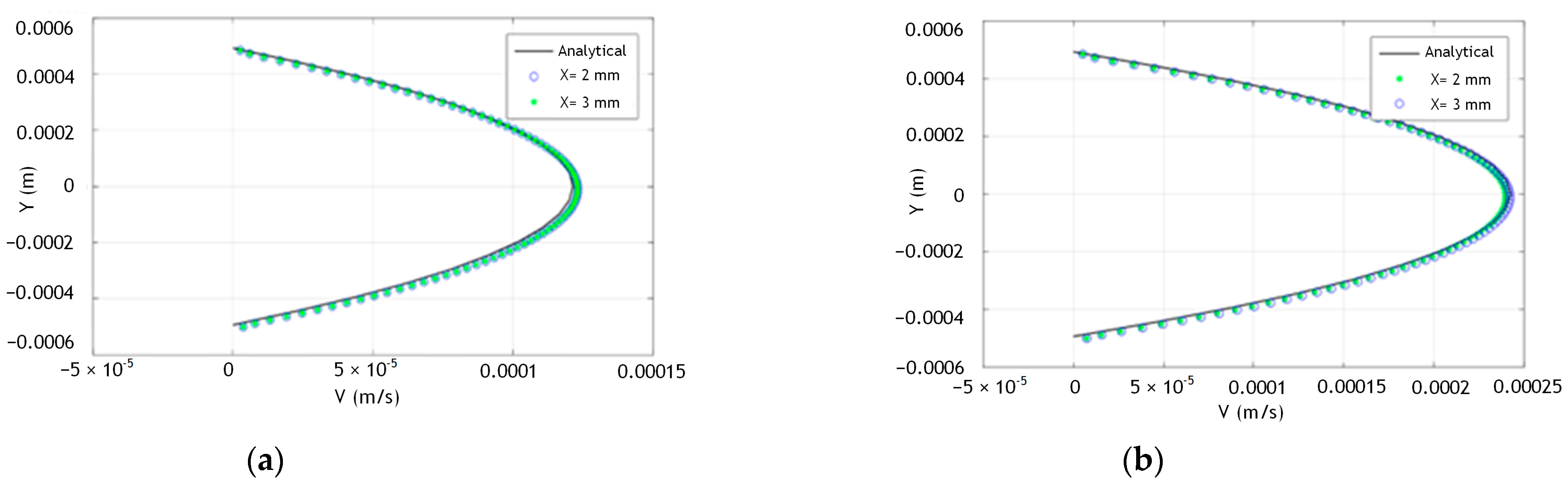
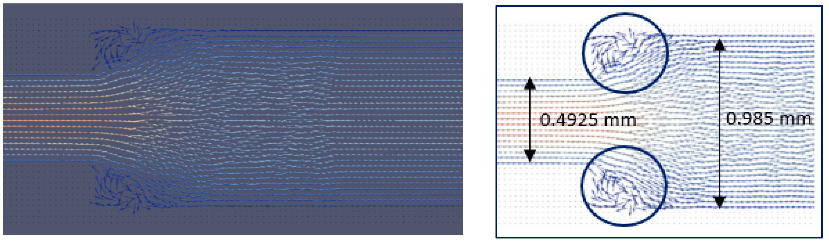
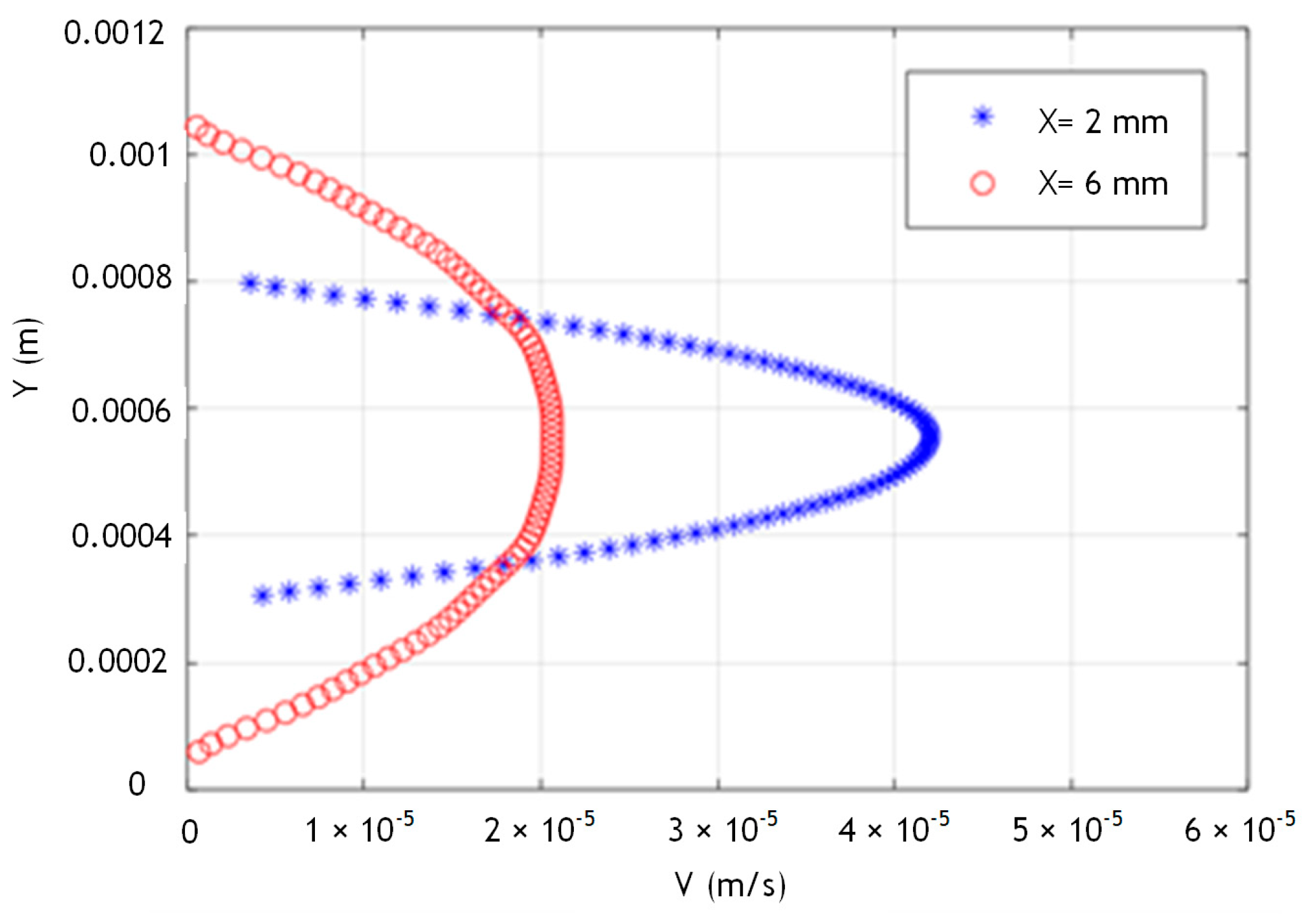
3.1.2. Two-Dimensional Sudden Expansion
3.1.3. Two-Dimensional Sudden Expansion/Contraction
3.2. Three-Dimensional Flows
3.2.1. Fully Developed Flow in a Square Duct of Constant Cross-Sectional Area
Poiseuille Number, the Relation f vs. Re
3.2.2. Developing Flow in a Square Microduct of Constant Cross-Sectional Area
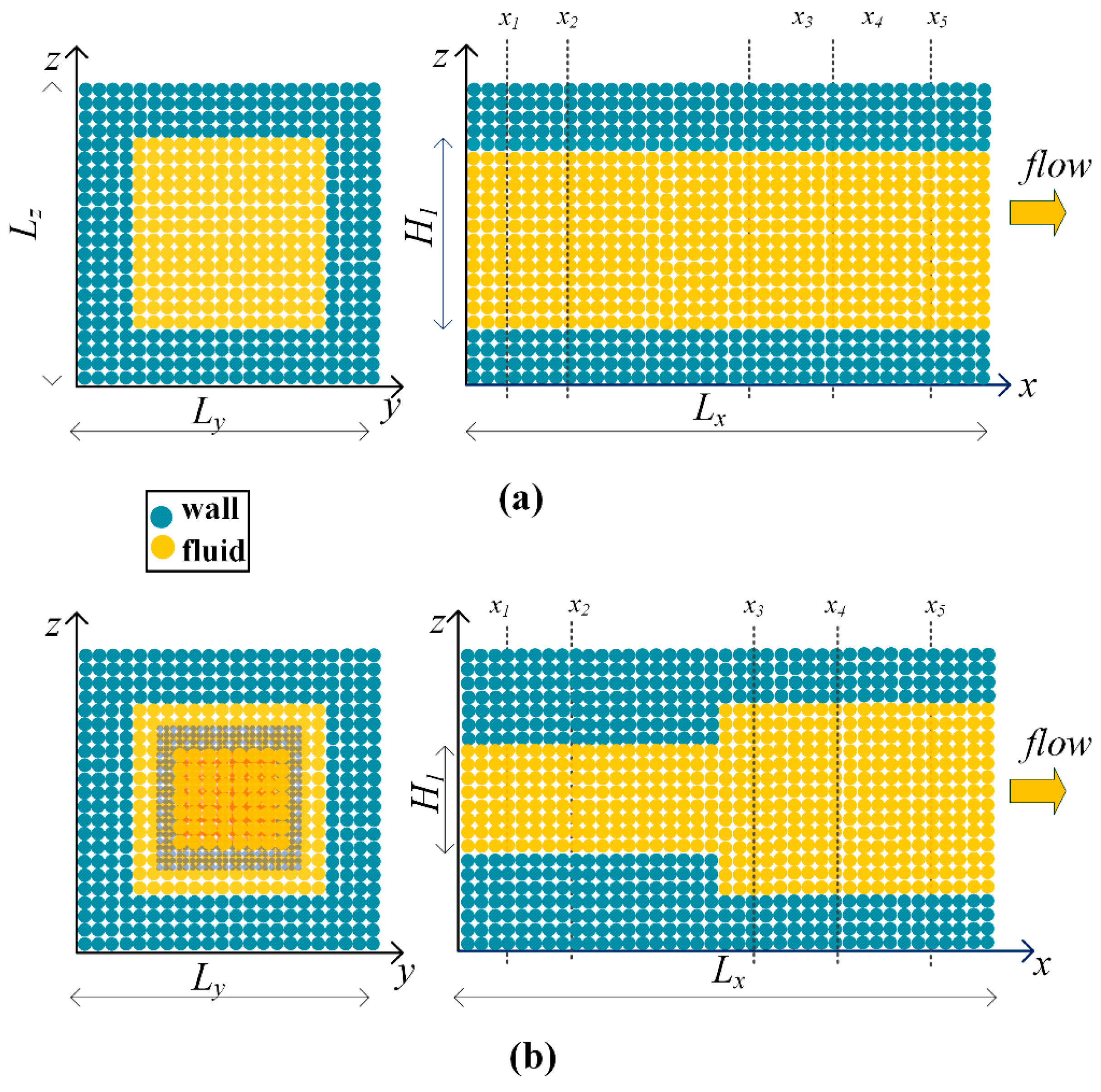
3.2.3. Three-Dimensional Microchannel with Sudden Expansion
3.2.4. Three-Dimensional Microchannels with Periodic Expansions/Contractions
4. Discussion
5. Conclusions
Author Contributions
Funding
Institutional Review Board Statement
Informed Consent Statement
Data Availability Statement
Conflicts of Interest
References
- Groenenboom, P.; Cartwright, B.; McGuckin, D.; Amoignon, O.; Mettichi, M.; Gargouri, Y.; Kamoulakos, A. Numerical Studies and industrial applications of the hybrid SPH-fe method. Comput. Fluids 2019, 184, 40–63. [Google Scholar] [CrossRef]
- Shadloo, M.S.; Oger, G.; Le Touzé, D. Smoothed particle hydrodynamics method for fluid flows, towards industrial applications: Motivations, current state, and challenges. Comput. Fluids 2016, 136, 11–34. [Google Scholar] [CrossRef]
- Patino-Narino, E.A.; Idagawa, H.S.; de Lara, D.S.; Savu, R.; Moshkalev, S.A.; Ferreira, L.O. Smoothed particle hydrodynamics simulation: A tool for accurate characterization of microfluidic devices. J. Eng. Math. 2019, 115, 183–205. [Google Scholar] [CrossRef]
- Kalteh, M.; Abbassi, A.; Saffar-Avval, M.; Harting, J. Eulerian–eulerian two-phase numerical simulation of nanofluid laminar forced convection in a microchannel. Int. J. Heat Fluid Flow 2011, 32, 107–116. [Google Scholar] [CrossRef]
- Sofos, F.; Chatzoglou, E.; Liakopoulos, A. An assessment of SPH simulations of sudden expansion/contraction 3-D channel flows. Comput. Part. Mech. 2021, 9, 101–115. [Google Scholar] [CrossRef]
- Zhang, Z.L.; Walayat, K.; Chang, J.Z.; Liu, M.B. Meshfree modeling of a fluid-particle two-phase flow with an improved SPH method. Int. J. Numer. Methods Eng. 2018, 116, 530–569. [Google Scholar] [CrossRef]
- Monaghan, J.J.; Gingold, R.A. Shock simulation by the Particle Method SPH. J. Comput. Phys. 1983, 52, 374–389. [Google Scholar] [CrossRef]
- Monaghan, J.J. Smoothed particle hydrodynamics. Annu. Rev. Astron. Astrophys. 1992, 30, 543–574. [Google Scholar] [CrossRef]
- Nasar, A.M.A.; Fourtakas, G.; Lind, S.J.; Rogers, B.D.; Stansby, P.K.; King, J.R.C. High-order velocity and pressure wall boundary conditions in Eulerian Incompressible SPH. J. Comput. Phys. 2021, 434, 109793. [Google Scholar] [CrossRef]
- Vacondio, R.; Altomare, C.; De Leffe, M.; Hu, X.; Le Touzé, D.; Lind, S.; Marongiu, J.-C.; Marrone, S.; Rogers, B.D.; Souto-Iglesias, A. Grand challenges for smoothed particle hydrodynamics numerical schemes. Comput. Part. Mech. 2020, 8, 575–588. [Google Scholar] [CrossRef]
- Plimpton, S. Fast parallel algorithms for short-range molecular dynamics. J. Comput. Phys. 1995, 117, 1–19. [Google Scholar] [CrossRef]
- Pivkin, I.V.; Caswell, B.; Karniadakis, G.E. Dissipative Particle Dynamics. Rev. Comput. Chem. 2010, 27, 85–110. [Google Scholar] [CrossRef]
- Ellero, M.; Español, P. Everything you always wanted to know about SDPD⋆ (⋆but were afraid to ask). Appl. Math. Mech. 2017, 39, 103–124. [Google Scholar] [CrossRef]
- Perdikaris, P.; Grinberg, L.; Karniadakis, G.E. Multiscale modeling and simulation of Brain Blood Flow. Phys. Fluids 2016, 28, 021304. [Google Scholar] [CrossRef]
- Albano, A.; le Guillou, E.; Danzé, A.; Moulitsas, I.; Sahputra, I.H.; Rahmat, A.; Duque-Daza, C.A.; Shang, X.; Ng, K.C.; Ariane, M.; et al. How to modify LAMMPS: From the prospective of a particle method researcher. ChemEngineering 2021, 5, 30. [Google Scholar] [CrossRef]
- Liakopoulos, A.; Sofos, F.; Karakasidis, T.E. Darcy-Weisbach friction factor at the nanoscale: From Atomistic calculations to continuum models. Phys. Fluids 2017, 29, 052003. [Google Scholar] [CrossRef]
- Sofos, F.; Karakasidis, T.E.; Liakopoulos, A. Fluid flow at the nanoscale: How fluid properties deviate from the bulk. Nanosci. Nanotechnol. Lett. 2013, 5, 457–460. [Google Scholar] [CrossRef]
- Jacob, B.; Drawert, B.; Yi, T.-M.; Petzold, L. An arbitrary lagrangian eulerian smoothed particle hydrodynamics (Ale-SPH) method with a boundary volume fraction formulation for fluid-structure interaction. Eng. Anal. Bound. Elem. 2021, 128, 274–289. [Google Scholar] [CrossRef]
- Lyu, H.-G.; Sun, P.-N. Further enhancement of the particle shifting technique: Towards better volume conservation and particle distribution in SPH simulations of violent free-surface flows. Appl. Math. Model. 2022, 101, 214–238. [Google Scholar] [CrossRef]
- Marrone, S.; Antuono, M.; Colagrossi, A.; Colicchio, G.; Le Touzé, D.; Graziani, G. Δ-SPH model for simulating violent impact flows. Comput. Methods Appl. Mech. Eng. 2011, 200, 1526–1542. [Google Scholar] [CrossRef]
- Khayyer, A.; Shimizu, Y.; Gotoh, T.; Gotoh, H. Enhanced resolution of the continuity equation in explicit weakly compressible SPH simulations of incompressible free-surface fluid flows. Appl. Math. Model. 2023, 116, 84–121. [Google Scholar] [CrossRef]
- Monaghan, J.J. Simulating free surface flows with SPH. J. Comput. Phys. 1994, 110, 399–406. [Google Scholar] [CrossRef]
- Morris, J.P.; Fox, P.J.; Zhu, Y. Modeling low Reynolds Number Incompressible flows using SPH. J. Comput. Phys. 1997, 136, 214–226. [Google Scholar] [CrossRef]
- Zheng, X.; Ma, Q.; Shao, S. Study on SPH viscosity term formulations. Appl. Sci. 2018, 8, 249. [Google Scholar] [CrossRef]
- Oger, G.; Doring, M.; Alessandrini, B.; Ferrant, P. An improved SPH method: Towards higher order Convergence. J. Comput. Phys. 2007, 225, 1472–1492. [Google Scholar] [CrossRef]
- Colagrossi, A.; Landrini, M. Numerical simulation of interfacial flows by smoothed particle hydrodynamics. J. Comput. Phys. 2003, 191, 448–475. [Google Scholar] [CrossRef]
- Adami, S.; Hu, X.Y.; Adams, N.A. A generalized wall boundary condition for smoothed particle hydrodynamics. J. Comput. Phys. 2012, 231, 7057–7075. [Google Scholar] [CrossRef]
- Chen, C.; Zhang, A.M.; Chen, J.Q.; Shen, Y.M. SPH simulations of water entry problems using an improved boundary treatment. Ocean. Eng. 2021, 238, 109679. [Google Scholar] [CrossRef]
- Domínguez, J.M.; Fourtakas, G.; Altomare, C.; Canelas, R.B.; Tafuni, A.; García-Feal, O.; Martínez-Estévez, I.; Mokos, A.; Vacondio, R.; Crespo, A.J.C.; et al. DualSPHysics: From Fluid Dynamics to multiphysics problems. Comput. Part. Mech. 2021, 9, 867–895. [Google Scholar] [CrossRef]
- Liakopoulos, A. Fluid Mechanics, 2nd ed.; Tziolas Publication: Athina, Greece, 2019. [Google Scholar]
- Liakopoulos, A.; Sofos, F.; Karakasidis, T.E. Friction factor in nanochannel flows. Microfluid. Nanofluid. 2016, 20, 24. [Google Scholar] [CrossRef]
- White, F.M. Viscous Fluid Flow; McGraw-Hill: New York, NY, USA, 2006. [Google Scholar]
- Chatzoglou, E.; Liakopoulos, A. Hydraulic Jump Simulation via Smoothed Particle Hydrodynamics: A Critical Review. In Proceedings of the 39th IAHR World Congress, Granada, Spain, 19–24 June 2022. [Google Scholar]
- Chatzoglou, E.; Liakopoulos, A. Simulation of Open Channel Flow Control by Smoothed Particle Hydrodynamics. In Proceedings of the International Conference on Protection and Restoration of the Environment XVI, Kalamata, Greece, 5–8 July 2022. [Google Scholar]
- English, A.; Domínguez, J.M.; Vacondio, R.; Crespo, A.J.C.; Stansby, P.K.; Lind, S.J.; Chiapponi, L.; Gómez-Gesteira, M. Modified dynamic boundary conditions (MDBC) for general-purpose smoothed particle hydrodynamics (SPH): Application to tank sloshing, dam break and Fish Pass Problems. Comput. Part. Mech. 2021, 9, 1–15. [Google Scholar] [CrossRef]
- Liu, M.B.; Liu, G.R. Meshfree particle simulation of micro channel flows with surface tension. Comput. Mech. 2004, 35, 332–341. [Google Scholar] [CrossRef]
- Liakopoulos, A. Computation of high speed turbulent boundary-layer flows using The k-ε turbulence model. Int. J. Numer. Methods Fluids 1985, 5, 81–97. [Google Scholar] [CrossRef]
- Fourtakas, G.; Rogers, B.D. Modelling multi-phase liquid-sediment scour and resuspension induced by rapid flows using smoothed particle hydrodynamics (SPH) accelerated with a graphics processing unit (GPU). Adv. Water Resour. 2016, 92, 186–199. [Google Scholar] [CrossRef]


| Case | Poiseuille | Developing Flow | Sudden Expansion | Expansion/Contraction |
|---|---|---|---|---|
| Np | 10,000 | 10,060 | 10,340 | 15,300 |
| dp (m) | 2.00 × 10⁻⁵ | 2.00 × 10⁻⁵ | 2.98 × 10⁻⁵ | 2.98 × 10⁻⁵ |
| (m2/s) | 1.00 × 10⁻⁶ | 1.00 × 10⁻⁶ | 1.00 × 10⁻⁶ | 1.00 × 10⁻⁶ |
| BCs at solid wall | DBC | DBC | DBC | DBC |
| BCs in x-direction | Periodic | Inlet/outlet | Inlet/outlet | Periodic |
| Force per unit mass (m/s2) | gx = 0.001 | gx = 0.0 | gx = 0.0 | gx = 0.001 |
| Time Integration | Verlet | Verlet | Symplectic | Symplectic |
| Simulation time (s) | 5 | 5 | 20 | 30 |
| GPU time (min) | 2.1 | 2.5 | 10 | 8 |
| Baseline Simulation | SPH | Analytical | Rel. Diff. (%) |
|---|---|---|---|
| Periodic BCs | 0.48 | 0.49 | 2.04% |
| Inlet/outlet BC with buffer zones | 0.48 | 0.49 | 2.04% |
| Case | Const. C.S. (A) | Const. C.S. (B) | Sudden Expansion | Expan./Contr. |
|---|---|---|---|---|
| Np | 216,480 | 308,788 | 581,040 | 897,334 |
| dp (m) | 2.98 × 10⁻⁵ | 2.98 × 10⁻⁵ | 2.98 × 10⁻⁵ | 2.98 × 10⁻⁵ |
| (m2/s) | 1.00 × 10⁻⁶ | 1.00 × 10⁻⁶ | 1.00 × 10⁻⁶ | 1.00 × 10⁻⁶ |
| BCs at solid walls | DBC | DBC | DBC | DBC |
| BCs in x-direction | Periodic | Inlet/outlet | Inlet/outlet | Periodic |
| Force per unit mass (m/s2) | gx = 0.001 | gx = 0.0 | gx = 0.0 | gx = 0.001 |
| Time integration | Symplectic | Symplectic | Symplectic | Symplectic |
| T (s) | 20 | 50 | 60 | 50 |
| GPU time (min) | 13.6 | 24.6 | 38.85 | 51 |
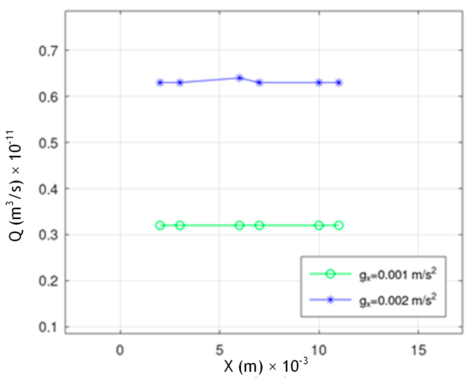
| x (mm) | gx = 0.001 m/s2 | gx = 0.002 m/s2 | ||
|---|---|---|---|---|
| 2 | 1.31 | 0.32 | 2.6 | 0.63 |
| 3 | 1.31 | 0.32 | 2.6 | 0.63 |
| 6 | 0.33 | 0.32 | 0.66 | 0.64 |
| 7 | 0.33 | 0.32 | 0.65 | 0.63 |
| 10 | 1.30 | 0.32 | 2.58 | 0.63 |
| 11 | 1.30 | 0.32 | 2.58 | 0.63 |
Disclaimer/Publisher’s Note: The statements, opinions and data contained in all publications are solely those of the individual author(s) and contributor(s) and not of MDPI and/or the editor(s). MDPI and/or the editor(s) disclaim responsibility for any injury to people or property resulting from any ideas, methods, instructions or products referred to in the content. |
© 2023 by the authors. Licensee MDPI, Basel, Switzerland. This article is an open access article distributed under the terms and conditions of the Creative Commons Attribution (CC BY) license (https://creativecommons.org/licenses/by/4.0/).
Share and Cite
Chatzoglou, E.; Liakopoulos, A.; Sofos, F. Smoothed Particle Hydrodynamics-Based Study of 3D Confined Microflows. Fluids 2023, 8, 137. https://doi.org/10.3390/fluids8050137
Chatzoglou E, Liakopoulos A, Sofos F. Smoothed Particle Hydrodynamics-Based Study of 3D Confined Microflows. Fluids. 2023; 8(5):137. https://doi.org/10.3390/fluids8050137
Chicago/Turabian StyleChatzoglou, Efstathios, Antonios Liakopoulos, and Filippos Sofos. 2023. "Smoothed Particle Hydrodynamics-Based Study of 3D Confined Microflows" Fluids 8, no. 5: 137. https://doi.org/10.3390/fluids8050137