Article

Comparison of Vortex Cut and Vortex Ring Models for Toroidal Bubble Dynamics in Underwater Explosions

1
College of Shipbuilding Engineering, Harbin Engineering University, Harbin 150001, China
2
The 1st Research Laboratory, Wuhan Second Ship Design and Research Institute, Wuhan 430200, China
3
Heilongjiang Province Key Laboratory of Nuclear Power System & Equipment, Harbin Engineering University, Harbin 150001, China
*
Author to whom correspondence should be addressed.
Fluids 2023, 8(4), 131; https://doi.org/10.3390/fluids8040131
Submission received: 25 February 2023 / Revised: 27 March 2023 / Accepted: 11 April 2023 / Published: 13 April 2023
(This article belongs to the Special Issue Numerical Modeling and Experimental Studies of Two-Phase Flows)

Abstract

:
The jet impact from a collapsing bubble is an important mechanism of structural damage in underwater explosions and cavitation erosion. The Boundary Integral Method (BIM) is widely used to simulate nonspherical bubble dynamic behaviors due to its high accuracy and efficiency. However, conventional BIM cannot simulate toroidal bubble dynamics, as the flow field transforms from single-connected into double-connected. To overcome this problem, vortex cut and vortex ring models can be used to handle the discontinuous potential on the toroidal bubble surface. In this work, we compare these two models applied to toroidal bubble dynamics in a free field and near a rigid wall in terms of bubble profile, bubble gas pressure, and dynamic pressure induced by the bubble, etc. Our results show that the two models produce comparable outcomes with a sufficient number of nodes in each. In the axisymmetric case, the vortex cut model is more efficient than the vortex ring model. Moreover, we found that both models improve in self-consistency as the number of bubble surface elements (N) increases, with N = 300 representing an optimal value. Our findings provide insights into the numerical study of toroidal bubble dynamics, which can enhance the selection and application of numerical models in research and engineering applications.

1. Introduction

Various types of bubbles in nature and industrial applications have been extensively studied. These include cavitation bubbles generated by snapping shrimp [1,2], vapor bubbles leading to cavitation erosion [3], bubbles triggered by underwater explosions [4,5,6], and airgun bubbles generated during resource exploration [7,8]. Previous works have proposed several analytical methods to understand the dynamics of spherical bubbles [9,10,11,12,13], such as the Rayleigh–Plesset equation [9,11] and the Keller equation [12]. Prosperetti and Lezzi [13,14] derived the one-parameter family equation of the first and second-order Mach number, respectively. The first-order equation can be simplified to the Keller or Herring form with different coefficients. Zhang et al. [15] established a unified theory for spherical bubble dynamics, which takes into account the effects of viscosity, boundaries, bubble interaction, gravity, bubble migration, fluid compressibility, and more. In reality, most bubbles become nonspherical and the high-speed water jet forms under gravity or induced by varieties of boundaries. Such jets carry up to 31% of the energy of the bubble system [16] and thus can cause much more concentrated damage in underwater explosions. Thus, nonspherical bubbles are of great research value. Blake et al. [17] solved the boundary integral equation with linear elements to obtain the velocity of the bubble surface and simulate the bubble oscillating process. The same authors [18] used the method mentioned above to study the interaction between a cavitation bubble and free surfaces. Later, the Boundary Integral Method (BIM) became very popular in the community of bubble dynamics. Chahine and his collaborators [19] carried out Three Dimensional (3D) simulations for bubble interactions with underwater structures and floating bodies. Khoo and his collaborators [20,21] further improved the 3D BIM model and performed extensive studies for underwater explosion bubbles. Li et al. [22] used 3D BIM to study the strong interaction between a pulsating bubble and a movable sphere. Zhang and his collaborators [23,24] also studied the nonlinear interaction between oscillating bubbles and various boundaries. Manmi et al. [25] used BIM to investigate the dynamics of a microbubble oscillating between two curved rigid plates in a planar acoustic field. Three-dimensional dynamics of a transient bubble oscillating inside a rigid corner were studied numerically by Dadvand et al. [26] using BIM. Wang et al. [27,28] proposed weakly compressible BIM and applied it to investigate nonspherical bubble dynamics of underwater explosions.
Recently, Li et al. [29] discovered that the weakly compressible BIM [30] and an all-Mach method (AMM) produced very similar results when Ma was below 0.3, and the incompressible BIM could be safely used with appropriate initial parameter settings. However, the traditional BIM cannot simulate bubble oscillations after jet impact since the flow domain becomes doubly connected. To simulate toroidal bubbles, Lundgren and Mansour et al. [31] divided the velocity potential into two parts: a continuous part from a smooth dipole distribution over the bubble surface and a discontinuous part related to a vortex ring. Best [32] proposed a cut created by the impact, whose geometry can change as a material surface. In this model, the domain can still be considered singly connected after impact. Later, Best [33] introduced a relocated cut that is re-mapped to a simple disc and follows each advancement of the flow. Additionally, Zhang et al. [34] introduced a vortex sheet to divide the jet from the surrounding flow field. Wang et al. [35] proposed a vortex ring model, which can also be applied to simulate three-dimensional problems. Later, Zhang et al. [36] developed a three-dimensional vortex ring model based on the two-dimensional one.
To date, numerous studies have investigated nonspherical bubble dynamics using numerical approaches [37,38]. Various numerical methods, including the Finite Volume Method (FVM) [39,40,41,42], the Finite Element Method (FEM) [4,43,44,45], the Smoothed Particle Hydrodynamics (SPH) [46,47,48], and the Boundary Integral Method (BIM), have been used to understand bubble dynamics [49,50,51,52,53]. Among these, the BIM is widely used for its high computational efficiency and accuracy. In this context, it has become crucial to comprehensively compare these different models, which would provide an indispensable foundation for toroidal bubble dynamics research. Therefore, here, we conduct a comprehensive study of the vortex ring and vortex cut models based on the original axisymmetric BIM code. We adopt the two mentioned numerical models to simulate bubbles generated from underwater explosions (hereafter, ‘UNDEX bubbles’) in the toroidal phase. We explore the characteristics and performances of each model in terms of CPU cost, convergence, and accuracy, as well as the toroidal bubble dynamics obtained from each model in terms of bubble profile, bubble gas pressure, and dynamic pressure induced by the bubble, etc.
The remainder of this study is organized as follows. In Section 2, we present an introduction to the BIM, the vortex cut model, and the vortex ring model. Validation and self-consistency analysis of the two models are conducted. In Section 3, we study toroidal bubbles in a free field or near a rigid wall and compare the results between the models. Finally, we present conclusions in Section 4.

2. Theories and Numerical Methods

2.1. Boundary Integral Method

The BIM has been widely used to research bubble dynamics as a high-efficiency numerical method [24,28,29,37,51,54,55], especially for nonspherical bubbles near boundaries. We assume the flow surrounding the bubble to be inviscid and irrotational. The Mach numbers of all cases presented herein are within 0.3, so we can safely use the incompressible BIM to study the nonspherical bubble dynamics with a proper setting of initial parameters [29]. The Peclet number (defined as R m 2 / T osi D , where T osi is the bubble period and D is the thermal diffusivity) in our work is O ( 10 8 ) . Thus, the bubble gas is considered to be adiabatic throughout the bubble life. We neglect heat and mass transfer across the bubble surface. As the maximum radius of a UNDEX bubble is O ( m ) , and the average velocity is O ( 10 m / s ) , the Reynolds number is greater than O ( 10 7 ) , and thus the viscosity of the surrounding liquid is negligible. Here, we define a cylindrical coordinate system ( r , θ , z ), in which the positive direction of the z axis is upward. The origin is set at the point of detonation. According to the above assumptions, the flow is governed by
2 ϕ = 0 .
where ϕ is the velocity potential.
According to the Green function, the boundary integral equation can be obtained to solve Equation (1):
λ ( r , t ) ϕ ( r , t ) = s ϕ ( q , t ) n G ( r , q ) ϕ ( q , t ) n G ( r , q ) dS ,
where λ is the solid angle, q is the source point, r is the field point, S denotes all boundaries, and / n is the normal outward derivative from the boundary. To study an explosion bubble in a free field and near an infinite rigid wall, the Green functions are written as
G ( r , q ) = 1 | r q | ,
G ( r , q ) = 1 | r q | + 1 | r q | ,
where q is the reflected image across the rigid wall of q .
The position of the bubble surface can be updated using the kinematic boundary condition:
d r d t = ϕ ,
where r denotes the position of the bubble surface. Based on the Bernoulli equation, the dynamic boundary condition is given by
d ϕ d t = 1 2 | ϕ | 2 + p p ρ g z ,
where p is the ambient pressure of the liquid at z = 0 , p is the liquid pressure at the bubble surface, g is the acceleration of gravity, and ρ denotes the density of the liquid, which is 1024 kg / m 3 in this paper. Equation (6) can be used to update the velocity potential at the bubble surface.
For explosion bubbles, the surface tension is ignorable because the Weber number is much larger than 1. Thus, according to the adiabatic equation, the liquid pressure p at the bubble surface can be obtained by
p = p b = p c + p 0 V 0 V κ ,
where p c refers to the vapor pressure, V is the bubble volume, and the subscript 0 denotes the initial state. κ is the adiabatic index, and κ = 1.25 for TNT charge.
The initial velocity of the bubble surface is 0. Following Klaseboer et al. [56], the initial bubble radius R 0 can be obtained by
1.39 × 10 5 p 3 W 4 π R m 3 κ 1 R 0 R m 3 ( κ 1 ) = κ 1 R 0 R m 3 1 ,
where W denotes the weight of the charge, and R m is the maximum bubble radius. Following Cole [57], R m can be obtained from empirical formulas.
In this paper, parameters are nondimensionalized for convenience. The superscript * denotes that the quantity is dimensionless. The ambient pressure of the liquid p (at the plane of z = 0 ), the maximum bubble radius R m , and the density of the liquid ρ are considered the pressure, length, and density scales, respectively. The stand-off, buoyancy, and strength parameters are thus defined as:
γ = L R m ,
δ = ρ g R m p ,
ϵ = p 0 p .
It is worth mentioning that the conventional BIM cannot simulate bubble oscillation after the jet impact because the flow domain becomes doubly connected. Two models based on the conventional BIM, the vortex cut model [32,34,58,59,60] and the vortex ring model [36,38,61], have been developed and widely used by researchers to study toroidal bubble dynamics. More details are given below.

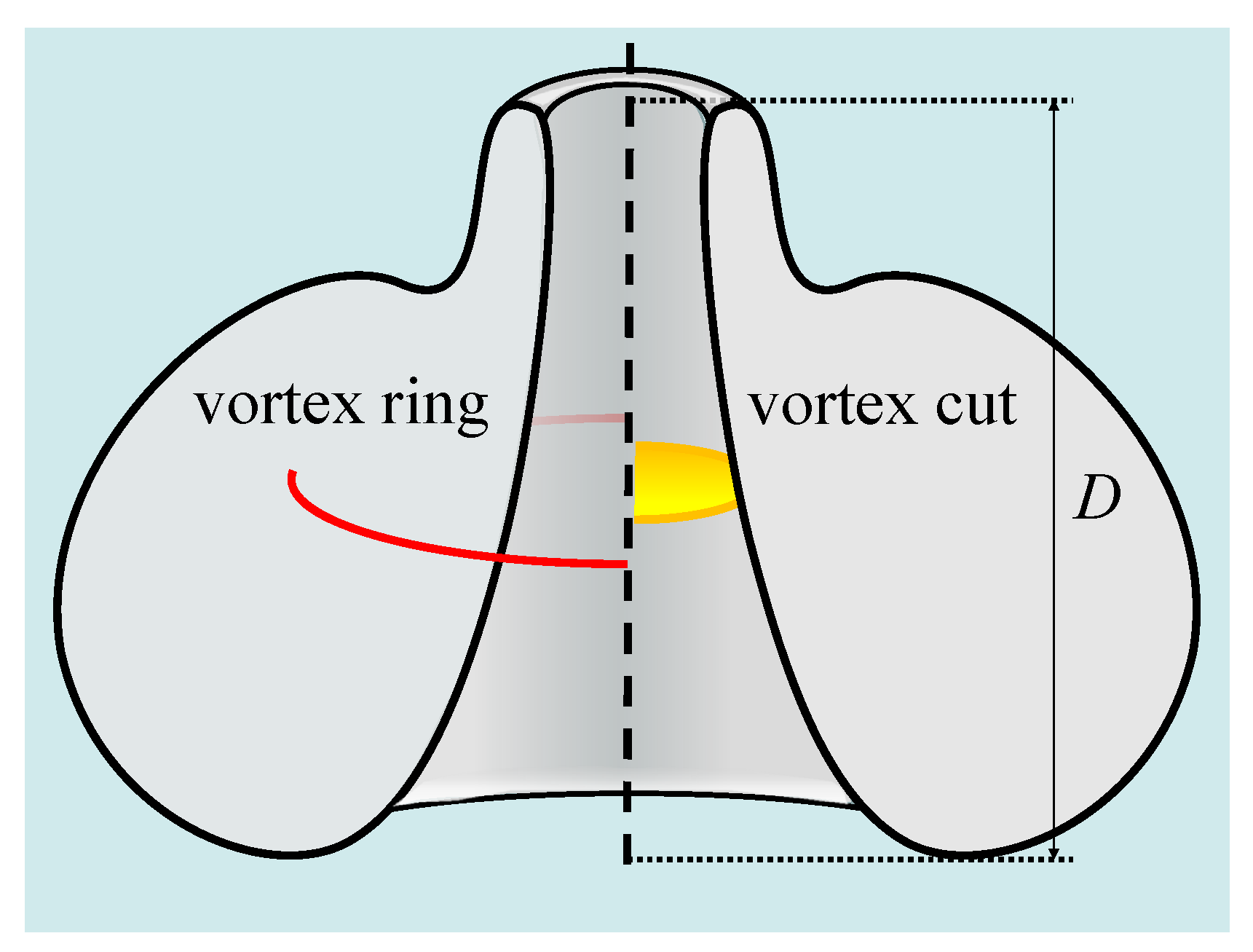
2.2. Vortex Cut Model

In the vortex cut model, a vortex cut T is introduced, including an upper surface T + and a lower surface T , thus the modified boundary integral equation [32] becomes
λ ( r , t ) ϕ ( r , t ) = s ϕ ( q , t ) n G ( r , q ) ϕ ( q , t ) n G ( r , q ) d S + T ϕ ( r , t ) n + G ( r , q ) ϕ + ( r , t ) n + G ( r , q ) d S + T ϕ ( r , t ) n G ( r , q ) ϕ ( r , t ) n G ( r , q ) d S ,
where / n + and / n denote the normal outward derivative from T + and T , respectively. Because / n + G ( r , q ) = / n G ( r , q ) , Equation (12) can be written as
λ ( r , t ) ϕ ( r , t ) = s ϕ ( q , t ) n G ( r , q ) ϕ ( q , t ) n G ( r , q ) d S Δ ϕ T n + G ( r , q ) d S ,
where Δ ϕ is the jump of potential ϕ across T. The position and shape of the vortex cut are arbitrary as long as Δ ϕ keeps constant.
The model is shown in the right part of Figure 1. In our model, we set an upper limit (80% of the bubble’s overall height) and a lower limit for the movement of the cut to keep the calculation stable. We set the cut at the lower limit initially. During the computation process, we reset the cut to the lower limit once it reaches the upper limit. Then the cut will continue moving along with the bubble surface in the limited region until the end of the calculation. Refer to Pearson et al. [58] for more details on cut shifting.
In the numerical model, we set T + and T as two cuts very close to each other for calculation, each of which connects with two adjacent elements at the bubble surface. The velocity potential and location of the bubble surface are updated by the kinematic and dynamic boundary conditions mentioned above.

2.3. Vortex Ring Model

In the vortex ring model, there exists a vortex ring in the bubble at ( a , c ) , as shown in the left part of Figure 1. The velocity potential ϕ is divided into two parts, the induced potential by the vortex ring ϕ v o r and the remnant potential ϕ r e . Accordingly, the velocity in the flow is decomposed into the induced velocity by the vortex ring u v o r and the remnant velocity u r e , which can be calculated according to the Biot–Savart law and the boundary integral equation, respectively. The Biot–Savart law can be expressed as
u v o r ( r , z ) = Γ 4 π C d l × r r 3 ,
where dl is the element of the vortex ring.
The induced velocity potential ϕ v o r can be obtained by using a semi-analytical method [62] with the known induced velocity u v o r :
ϕ v o r ( r , z ) = ( r , + ) ( r , z ) u v o r · e z d R z = Γ 4 π R z | R | 1 1 R r 2 e z · ( d l × R ) ,
ϕ v o r ( r , z ) = ( r , ) ( r , z ) u v o r · e z d R z = Γ 4 π R z | R | 1 1 R r 2 e z · ( d l × R ) ,
where the integration path is the vortex ring and l is the infinitesimal value on it. R refers to the vector from the center of the infinitesimal to ( r , z ) . Γ denotes the circulation of the vortex ring. It can be obtained from the jump in potential across the contact point during the jet impact process. e z is the unit vector of the z axis. Equations (14) and (15) are suitable for the case that ( r , z ) is above or below the vortex ring, respectively.
The remnant potential ϕ r e can be updated via the dynamic boundary condition mentioned above. The remnant velocity u r e can be updated via the boundary integral equation. Then, we can sum the remnant velocity u r e and the induced velocity u v o r , yielding the total velocity u.

3. Results

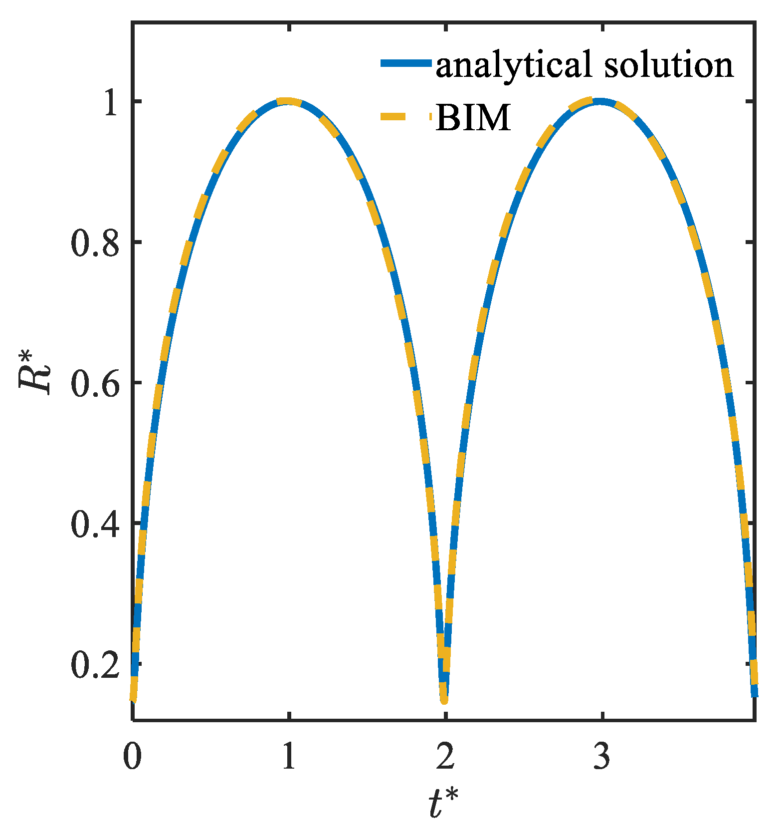
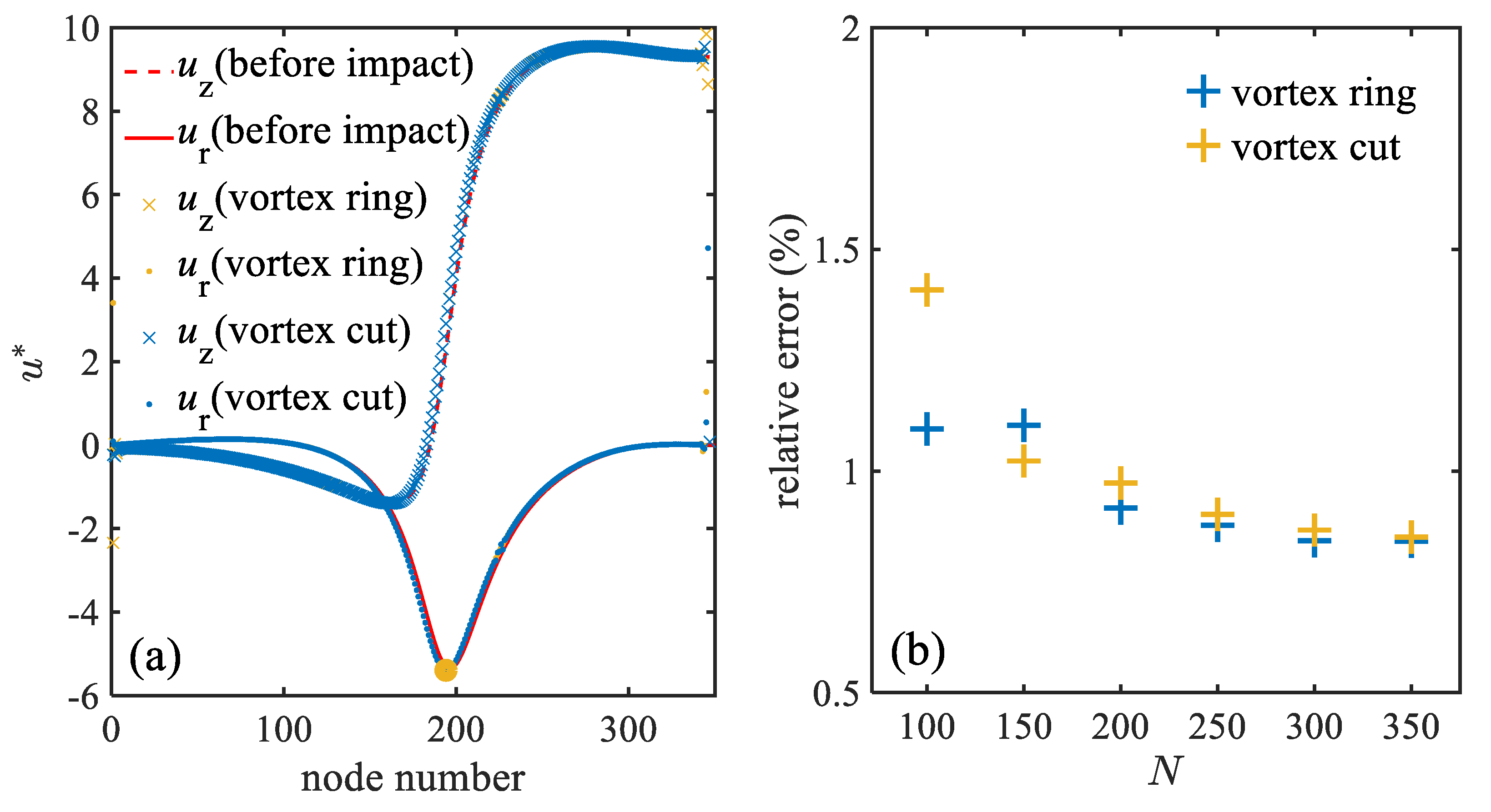
3.1. Verification Analysis

We validate the BIM code first. We compare the spherical bubble dynamics obtained from the BIM simulation and analytical solution [15]. The initial conditions of the case are set as: R 0 * = 0.15 , ϵ = 102.35 , and δ = 0 . Figure 2 shows the time evolution of the bubble radius in the first two bubble periods. No difference can be discerned between the two curves. The relative error of the maximum bubble radius is within 0.1%, which demonstrates the accuracy of our BIM model.
Next, we carry out a self-consistency analysis for the bubble surface velocity u r and u z with different element numbers of the bubble surface N. The initial conditions are set as: R 0 * = 0.15 , ϵ = 102.35 , and δ = 0.23 . We set N = 100 , 150, 200, 250, 300, and 350 for the bubble surface and compare the velocity of each node before and after jet impact (Figure 3). At N = 350 , the results of the two models are in excellent agreement with the velocities before the jet impact, except for the local position around the impact area. This suggests that each model has good self-consistency. Next, we study how the results change with N. We choose the node with the minimum u r in each case and calculate the relative deviation of u r before and after the impact moment. The velocity deviations of both u r and u z decrease as the number of bubble surface elements increases. The deviations reach the minimum values at N = 300 and remain constant after that. This demonstrates that the accuracy of both models improves as N increases, and achieves a convergence result at N = 300 .
The element number of the vortex cut m can also affect the calculation. We set 5, 6, 7, 8, 9, and 10 elements for the cut and find that the computational process is unstable at too small an m. We obtain a stable and convergent result at m = 8 in the test of the code. Thus, we set eight elements for the vortex cut in this paper unless otherwise indicated. As for the vortex ring model, we set 50, 100, 200, and 400 elements for the ring to test the computational efficiency. The run time increases with more vortex ring elements while the results reach convergence at 200 elements, so we set 200 elements for the vortex ring to reduce the CPU cost.

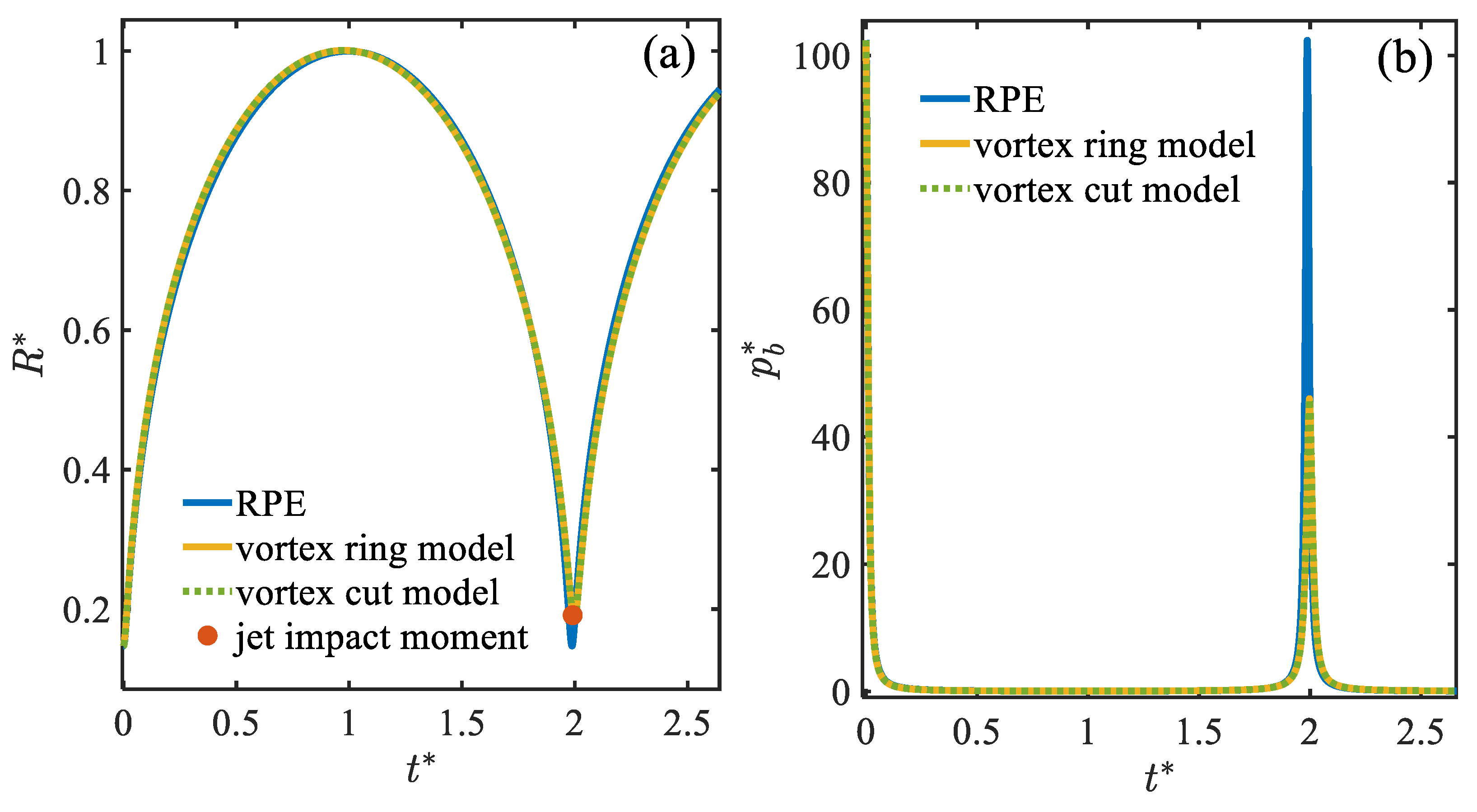
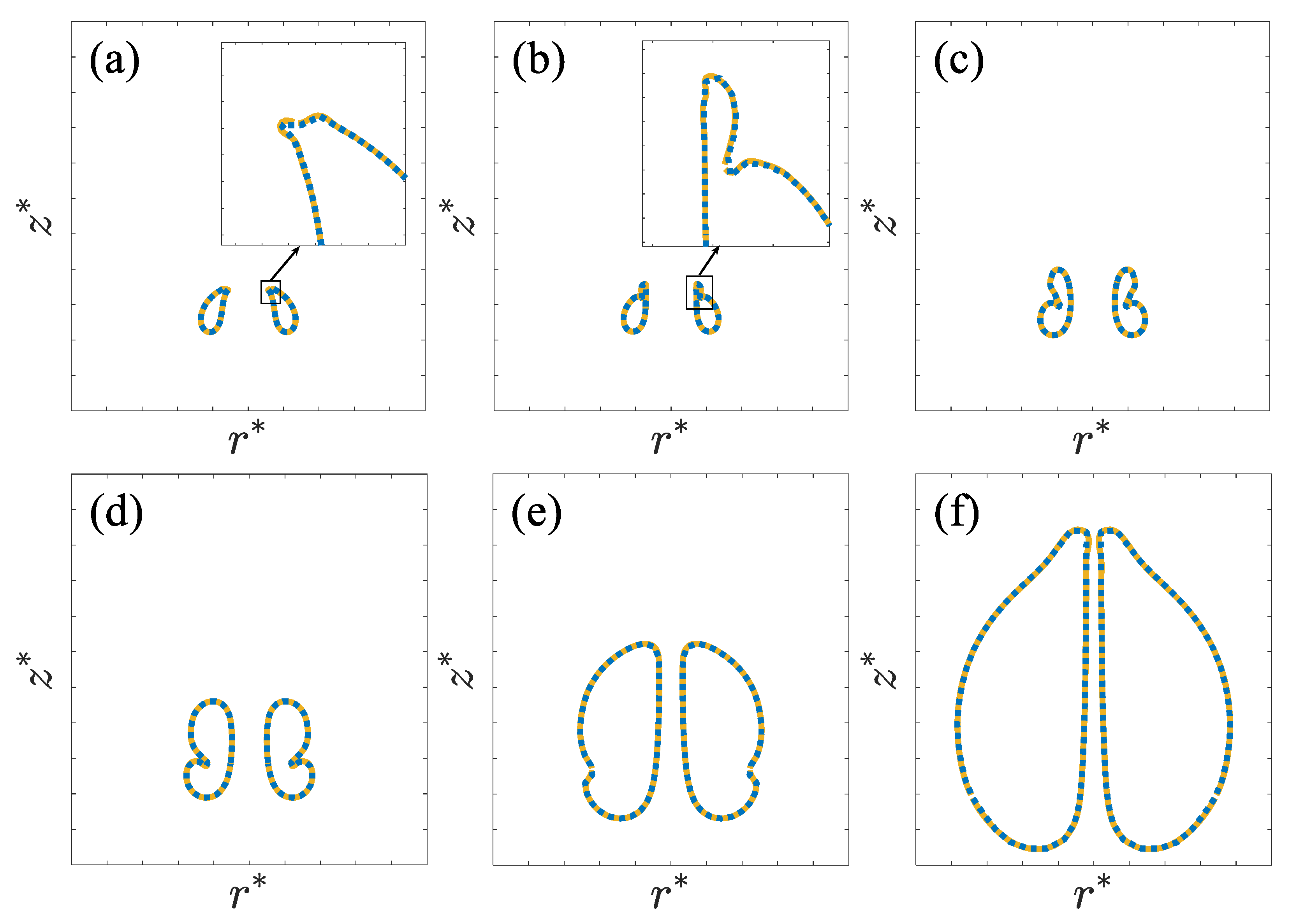
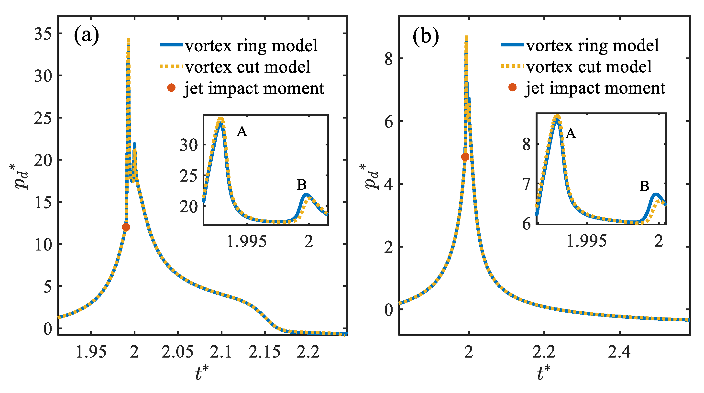
3.2. Toroidal Bubble in a Free Field

In this section, we apply both models to study UNDEX bubble dynamics in a free field. The initial conditions are set as: R 0 * = 0.15 , ϵ = 102.35 , and δ = 0.23 . Figure 4 demonstrates the time evolution of the bubble radius R * obtained from the Rayleigh–Plesset equation (RPE) and BIM. The jet impacts the bubble surface after the minimum bubble volume moment. The two results are in good agreement. Gravity is ignored in the RPE, so there is a difference in the minimum bubble radius between the RPE and BIM simulation, which is 24%. However, the two numerical calculation results perfectly coincide with each other. This implies that both models can predict toroidal bubble oscillations well in terms of bubble volume.
Next, we compare bubble gas pressure p b * obtained analytically and numerically for a better illustration of the bubble dynamics (Figure 4b). There is an obvious difference at the pressure peak, corresponding to the difference at the minimum bubble radius (shown in Figure 4a). The difference in the bubble pressure peak is 55%. This suggests that gravity plays a vital role in large-scale UNDEX bubbles, and theories of spherical bubbles are not useful for describing the detailed behaviors of nonspherical bubbles and the induced pressure waves. As expected, the results from the two models are in excellent agreement. This suggests the high similarity between the two models in regard to toroidal bubble dynamics in a free field.
Figure 5 compares the bubble profiles at different moments ( t * = 1.993, 2.000, 2.016, 2.044, 2.130, and 2.309). The results of the two models are identical. After the jet impact moment, the bubble surface remains smooth and gradually collapses to the minimum volume with an annular jet inward. Thereafter, the bubble expands with a protrusion on the top of the surface, and the annular jet moves downward along the bubble surface (frames b–d). Meanwhile, the water jet becomes thinner as the bubble expands to the maximum volume (frames e and f). All of the details are predicted well by both models, including the annular jet and the protrusion.
Next, we turn to the dynamic pressure in the flow field (Figure 6). In both models, two local pressure peaks are observed, marked A and B, which correspond to frames a and b in Figure 5, respectively. It is clear that the strong jet impact causes a growing protrusion at the top of the bubble. This leads to pressure peaks in the flow field. Similar phenomena and detailed analysis can be found in the study by Li et al. [61]. During the ascending and descending stages, the pressures calculated by the two approaches agree well with each other, with slight differences of 2.7% and 2.6% at local pressure peaks A and B, respectively. However, the pressure peaks are transient, so the comparison lacks universal significance. Next, we calculate the time integral of the dynamic pressure from the jet impact moment to t * = 2.2 . The difference in the pressure impulse is negligible at 0.6%. At field point (2, 0), the results are virtually identical between the two models except for the two local pressure peaks. The differences are 1.7% and 2.5%, respectively. The difference in the pressure impulse calculated from the jet impact moment to t * = 2.2 is 0.4%.
In sum, an overall match is obtained for toroidal bubble dynamics in a free field, except for some tiny differences in dynamic pressure in the flow field.

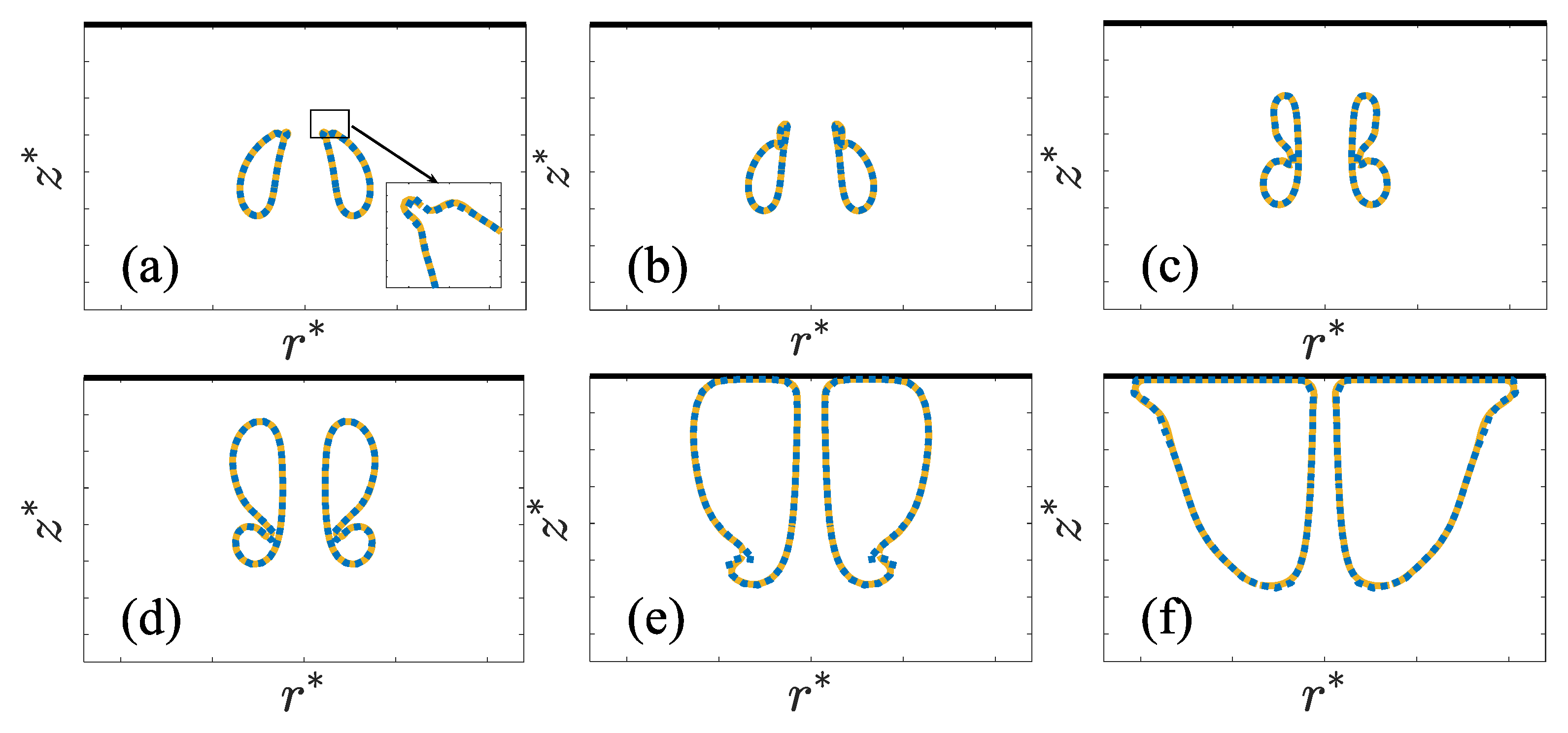
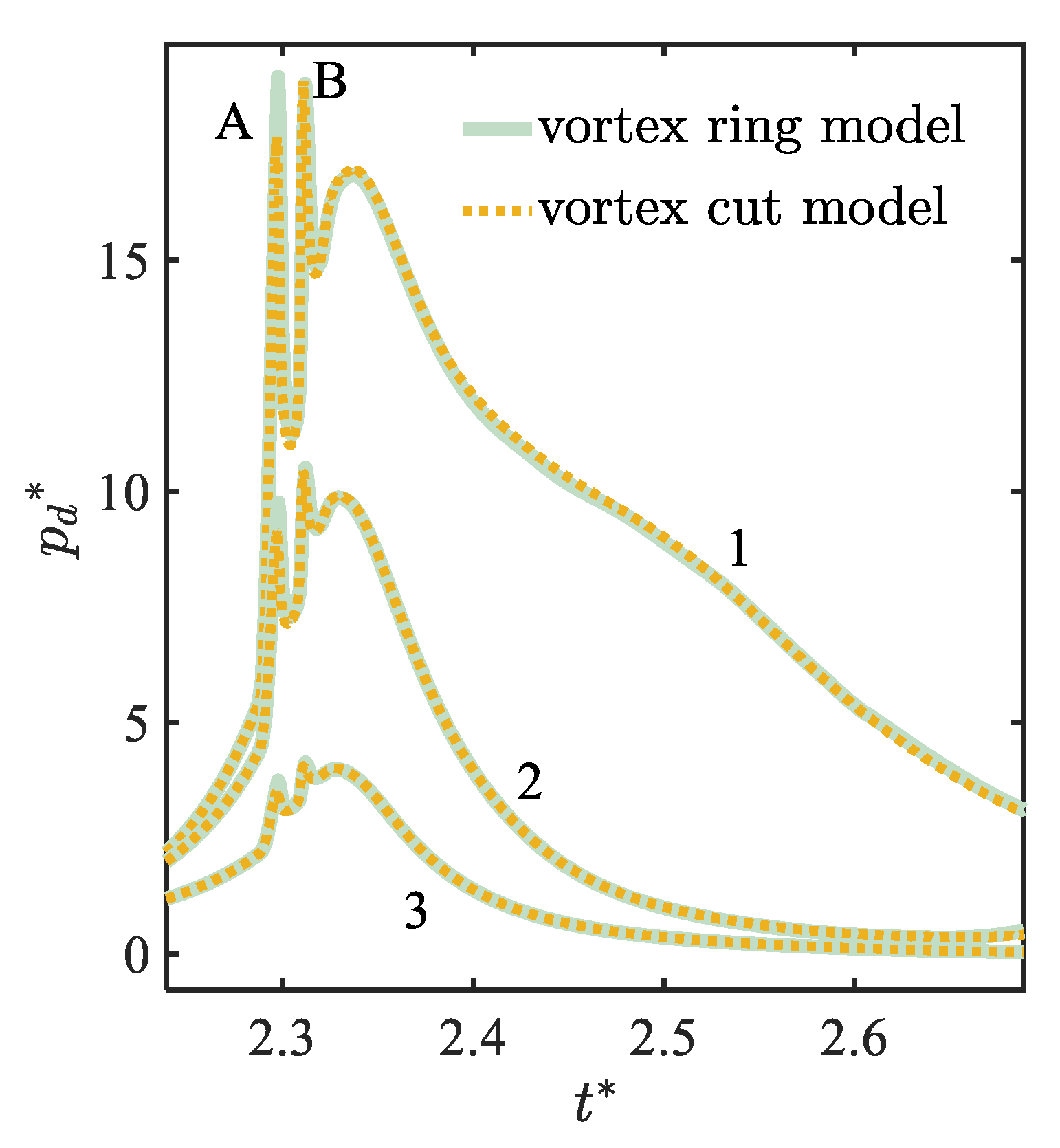
3.3. Toroidal Bubble near a Rigid Wall

Next, we study the toroidal bubble dynamics near an infinite rigid wall using the two numerical models. The initial conditions are set as: R 0 * = 0.19 , ϵ = 50.28 , δ = 0.11 and γ = 1.4 . Figure 7 compares the bubble profiles was obtained from the two models at t * = 2.298 , 2.312, 2.359, 2.414, 2.616, and 2.853. A growing protrusion forms at the top of the toroidal bubble in the initial stage (frames a–c) while the bubble moves towards the rigid wall. An annular water jet forms and develops inwards (frames c and d). After the bubble reaches the wall, its surface is flattened, and the contact surface gradually enlarges (frames e and f). The results of the two models are identical.
In the study of a UNDEX bubble near a solid boundary, the dynamic pressure induced at the boundary is of great significance and can be used to evaluate the damage ability. The evolution of dynamic pressure at the rigid wall p d * obtained by each model is shown in Figure 8. The moments of A and B correspond to frame a and b in Figure 7. After the water jet penetrates the upper surface of the bubble, p d * increases rapidly and reaches two local peaks (marked A and B). After the bubble becomes toroidal, the high-speed water jet violently impacts the rigid wall, which leads to the pressure peaks. The results of the two models coincide well except for some tiny differences in the pressure peaks (e.g., that at Peak A being 8.35% higher for the vortex ring model vs. the vortex cut model). The differences are 7.49% and 5.7% in group 2 and group 3, respectively. We integrate the dynamic pressures from the jet impact moment to t * = 2.65 to obtain the pressure impulse. The results of the two models are both 3.79. This demonstrates the excellent agreement between the two models.
Finally, the computational efficiency of each model is assessed. We run the codes for different computation time steps on a personal laptop with 11th Gen Intel (R) Core (TM) i5-1135G7 CPU at 1.40 GHz). As shown in Figure 9, the vortex cut model has a significant advantage over the vortex ring model. The average difference in CPU cost for the four groups of time steps is 36%.

4. Conclusions

In this paper, we employ the BIM to study UNDEX bubble dynamics. After jet impact, the flow field becomes doubly connected; thus, the vortex ring and vortex cut models are proposed to study the toroidal bubble dynamics. We discuss the efficiency and accuracy of the two models and compare the bubble dynamics obtained from them in terms of bubble radius, bubble gas, and pressure impulse. The main findings are as follows:
(1) The self-consistency of each model improves as the number of bubble surface elements N increases, and both are optimal at N = 300 . The computational process becomes more stable as the number of vortex ring and vortex cut elements increases.
(2) As for a bubble in a free field, the bubble radius and the bubble gas pressure obtained from RPE and the numerical models are compared. We find significant differences at the moment of minimum bubble volume. This suggests that the effect of gravity plays a vital role in large-scale UNDEX bubbles, and theories of spherical bubbles cannot be used to describe the detailed behaviors of nonspherical bubbles and the induced pressure waves. The two models coincide well at all time points. As for the dynamic pressure in the flow field, the two models have very close results with only slight differences at local pressure peaks.
(3) As for a bubble near an infinite rigid wall, the bubble oscillations are predicted well by the two numerical models. Regarding the dynamic pressure at the rigid wall, there are some differences at the pressure peaks of each model, which decrease with measuring-point distance from the center of the wall. However, the pressure peaks are transient, so the time integrals of pressure obtained from the two models are the same.
(4) The vortex ring model is more computationally demanding than the vortex cut model, with a 36% greater average CPU cost.

Author Contributions

Conceptualization, S.L.; methodology, S.L. and L.H.; software, S.L. and L.H.; validation, L.H.; formal analysis, L.H.; investigation, L.H. and S.L.; writing—original draft preparation, L.H.; writing—review and editing, T.Z., R.H. and S.L.; visualization, L.H. and S.L.; supervision, S.L.; funding acquisition, S.L., R.H. and D.Y. All authors have read and agreed to the published version of the manuscript.

Funding

This research was funded by the National Natural Science Foundation of China (12072087) and the Heilongjiang Provincial Natural Science Foundation of China (YQ2022E017).

Data Availability Statement

The data that support the findings of this study are available within the article.

Acknowledgments

The authors gratefully acknowledge A-Man Zhang for insightful discussions.

Conflicts of Interest

The authors declare no conflict of interest.

References

  1. Versluis, M.; Schmitz, B.; von der Heydt, A.; Lohse, D. How snapping shrimp snap: Through cavitating bubbles. Science 2000, 289, 2114–2117. [Google Scholar] [CrossRef] [PubMed] [Green Version]
  2. Lohse, D.; Schmitz, B.; Versluis, M. Snapping shrimp make flashing bubbles. Nature 2001, 413, 477–478. [Google Scholar] [CrossRef]
  3. Lindau, J.W.; Boger, D.A.; Medvitz, R.B.; Kunz, R.F. Propeller cavitation breakdown analysis. J. Fluids Eng. 2005, 127, 995–1002. [Google Scholar] [CrossRef]
  4. Liu, Y.L.; Zhang, A.M.; Tian, Z.L.; Wang, S.P. Investigation of free-field underwater explosion with Eulerian finite element method. Ocean Eng. 2018, 166, 182–190. [Google Scholar] [CrossRef]
  5. Ghoshal, R.; Mitra, N. Underwater explosion induced shock loading of structures: Influence of water depth, salinity and temperature. Ocean Eng. 2016, 126, 22–28. [Google Scholar] [CrossRef]
  6. Tian, Z.L.; Liu, Y.L.; Zhang, A.M.; Tao, L.B.; Chen, L. Jet development and impact load of underwater explosion bubble on solid wall. Appl. Ocean Res. 2020, 95, 102013. [Google Scholar] [CrossRef]
  7. Li, S.; Prosperetti, A.; van der Meer, D. Dynamics of a toroidal bubble on a cylinder surface with an application to geophysical exploration. Int. J. Multiph. Flow 2020, 129, 103335. [Google Scholar] [CrossRef]
  8. Li, S.; van der Meer, D.; Zhang, A.M.; Prosperetti, A.; Lohse, D. Modelling large scale airgun-bubble dynamics with highly non-spherical features. Int. J. Multiph. Flow 2020, 122, 103143. [Google Scholar] [CrossRef]
  9. Plesset, M.S. The dynamics of cavitation bubbles. J. Appl. Mech. 1949, 16, 277–282. [Google Scholar] [CrossRef]
  10. Brenner, M.P.; Hilgenfeldt, S.; Lohse, D. Single-bubble sonoluminescence. Rev. Mod. Phys. 2002, 74, 425. [Google Scholar] [CrossRef] [Green Version]
  11. Rayleigh, L. On the pressure developed in a liquid during the collapse of a spherical cavity. Lond. Edinb. Dublin Philos. Mag. J. Sci. 1917, 34, 94–98. [Google Scholar] [CrossRef]
  12. Keller, J.B.; Kolodner, I.I. Damping of underwater explosion bubble oscillations. J. Appl. Phys. 1956, 27, 1152–1161. [Google Scholar] [CrossRef]
  13. Prosperetti, A.; Lezzi, A. Bubble dynamics in a compressible liquid. Part 1. First-order theory. J. Fluid Mech. 1986, 168, 457–478. [Google Scholar] [CrossRef]
  14. Lezzi, A.; Prosperetti, A. Bubble dynamics in a compressible liquid. Part 2. Second-order theory. J. Fluid Mech. 1987, 185, 289–321. [Google Scholar] [CrossRef]
  15. Zhang, A.M.; Li, S.M.; Cui, P.; Li, S.; Liu, Y.L. A unified theory for bubble dynamics. Phys. Fluids 2023, 35, 033323. [Google Scholar] [CrossRef]
  16. Pearson, A.; Blake, J.R.; Otto, S.R. Jets in bubbles. J. Eng. Math. 2004, 48, 391–412. [Google Scholar] [CrossRef]
  17. Blake, J.R.; Taib, B.B.; Doherty, G. Transient cavities near boundaries. Part 1. Rigid boundary. J. Fluid Mech. 1986, 170, 479–497. [Google Scholar] [CrossRef]
  18. Blake, J.R.; Gibson, D.C. Cavitation bubbles near boundaries. Annu. Rev. Fluid Mech. 1987, 19, 99–123. [Google Scholar] [CrossRef]
  19. Kalumuck, K.M.; Duraiswami, R.; Chahine, G.L. Bubble dynamics fluid-structure interaction simulation by coupling fluid BEM and structural FEM codes. J. Fluids Struct. 1995, 9, 861–883. [Google Scholar] [CrossRef]
  20. Wang, C.; Khoo, B.C. An indirect boundary element method for three-dimensional explosion bubbles. J. Comput. Phys. 2004, 194, 451–480. [Google Scholar] [CrossRef]
  21. Klaseboer, E.; Hung, K.C.; Wang, C.; Wang, C.W.; Khoo, B.C.; Boyce, P.; Debono, S.; Charlier, H. Experimental and numerical investigation of the dynamics of an underwater explosion bubble near a resilient/rigid structure. J. Fluid Mech. 2005, 537, 387–413. [Google Scholar] [CrossRef]
  22. Li, S.; Zhang, A.M.; Han, R.; Ma, Q. 3D full coupling model for strong interaction between a pulsating bubble and a movable sphere. J. Comput. Phys. 2019, 392, 713–731. [Google Scholar] [CrossRef]
  23. Zhang, A.M.; Wu, W.B.; Liu, Y.L.; Wang, Q.X. Nonlinear interaction between underwater explosion bubble and structure based on fully coupled model. Phys. Fluids 2017, 29, 082111. [Google Scholar] [CrossRef] [Green Version]
  24. Han, R.; Zhang, A.M.; Tan, S.C.; Li, S. Interaction of cavitation bubbles with the interface of two immiscible fluids on multiple time scales. J. Fluid Mech. 2021, 932, A8. [Google Scholar] [CrossRef]
  25. Manmi, K.M.A.; Aziz, I.A.; Arjunan, A.; Saeed, R.K.; Dadvand, A. Three-dimensional oscillation of an acoustic microbubble between two rigid curved plates. J. Hydrodyn. 2021, 33, 1019–1034. [Google Scholar] [CrossRef]
  26. Dadvand, A.; Manmi, K.M.A.; Aziz, I.A. Three-dimensional bubble jetting inside a corner formed by rigid curved plates: Boundary integral analysis. Int. J. Multiph. Flow 2023, 158, 104308. [Google Scholar] [CrossRef]
  27. Curtiss, G.A.; Leppinen, D.M.; Wang, Q.X.; Blake, J.R. Ultrasonic cavitation near a tissue layer. J. Fluid Mech. 2013, 730, 245–272. [Google Scholar] [CrossRef]
  28. Wang, Q.X. Non-spherical bubble dynamics of underwater explosions in a compressible fluid. Phys. Fluids 2013, 25. [Google Scholar] [CrossRef]
  29. Li, S.; Saade, Y.; van der Meer, D.; Lohse, D. Comparison of Boundary Integral and Volume-of-Fluid methods for compressible bubble dynamics. Int. J. Multiph. Flow 2021, 145, 103834. [Google Scholar] [CrossRef]
  30. Wang, Q.X.; Blake, J.R. Non-spherical bubble dynamics in a compressible liquid. Part 1. Travelling acoustic wave. J. Fluid Mech. 2010, 659, 191–224. [Google Scholar] [CrossRef]
  31. Lundgern, T.S.; Mansour, N.N. Vortex ring bubbles. J. Mech. 1991, 224, 177–196. [Google Scholar]
  32. Best, J.P. The Dynamics of Underwater Explosions. Ph.D. Thesis, The University of Wollongong, Wollongong, Australia, 1991. [Google Scholar]
  33. Best, J.P. The Rebound of Toroidal Bubbles; Bubble Dynamics and Interface Phenomena; Springer: Berlin/Heidelberg, Germany, 1994. [Google Scholar]
  34. Zhang, S.; Duncan, J.H.; Chahine, G.L. The final stage of the collapse of a cavitation bubble near a rigid wall. J. Fluid Mech. 1993, 257, 147–181. [Google Scholar] [CrossRef]
  35. Wang, Q.X.; Yeo, K.S.; Khoo, B.C.; Lam, K.Y. Nonlinear interaction between gas bubble and free surface. Comput. Fluids 1996, 25, 607–628. [Google Scholar] [CrossRef]
  36. Zhang, Y.L.; Yeo, K.S.; Khoo, B.C.; Wang, C. 3D jet impact and toroidal bubbles. J. Comput. Phys. 2001, 166, 336–360. [Google Scholar] [CrossRef]
  37. Wang, Q.X. Multi-oscillations of a bubble in a compressible liquid near a rigid boundary. J. Fluid Mech. 2014, 745, 509–536. [Google Scholar] [CrossRef]
  38. Wang, Q.X.; Yeo, K.S.; Khoo, B.C.; Lam, K.Y. Vortex ring modelling of toroidal bubbles. Theor. Comput. Fluid Dyn. 2005, 19, 303–317. [Google Scholar] [CrossRef]
  39. Lauterborn, W.; Lechner, C.; Koch, M.; Mettin, R. Bubble models and real bubbles: Rayleigh and energy-deposit cases in a Tait-compressible liquid. IMA J. Appl. Math. 2018, 83, 556–589. [Google Scholar] [CrossRef]
  40. Li, T.; Wang, S.; Li, S.; Zhang, A.M. Numerical investigation of an underwater explosion bubble based on FVM and VOF. Appl. Ocean Res. 2018, 74, 49–58. [Google Scholar] [CrossRef]
  41. Li, T.; Zhang, A.M.; Wang, S.; Li, S.; Liu, W. Bubble interactions and bursting behaviors near a free surface. Phys. Fluids 2019, 31, 042104. [Google Scholar]
  42. Zeng, Q.; Cai, J. Three-dimension simulation of bubble behavior under nonlinear oscillation. Ann. Nucl. Energy 2014, 63, 680–690. [Google Scholar] [CrossRef]
  43. Tian, Z.L.; Liu, Y.L.; Zhang, A.M.; Tao, L.B. Energy dissipation of pulsating bubbles in compressible fluids using the Eulerian finite-element method. Ocean Eng. 2020, 196, 106714. [Google Scholar] [CrossRef]
  44. Liu, N.N.; Zhang, A.M.; Liu, Y.L.; Li, T. Numerical analysis of the interaction of two underwater explosion bubbles using the compressible Eulerian finite-element method. Phys. Fluids 2020, 32, 046107. [Google Scholar]
  45. He, M.; Liu, Y.L.; Zhang, S.; Zhang, A.M. Research on characteristics of deep-sea implosion based on Eulerian finite element method. Ocean Eng. 2022, 244, 110270. [Google Scholar] [CrossRef]
  46. Sun, P.; Le Touzé, D.; Oger, G.; Zhang, A.M. An accurate SPH Volume Adaptive Scheme for modeling strongly-compressible multiphase flows. Part 2: Extension of the scheme to cylindrical coordinates and simulations of 3D axisymmetric problems with experimental validations. J. Comput. Phys. 2021, 426, 109936. [Google Scholar] [CrossRef]
  47. Sun, P.N.; Pilloton, C.; Antuono, M.; Colagrossi, A. Inclusion of an acoustic damper term in weakly-compressible SPH models. J. Comput. Phys. 2023, 483, 112056. [Google Scholar] [CrossRef]
  48. Wang, P.; Zhang, A.M.; Fang, X.; Khayyer, A.; Meng, Z. Axisymmetric Riemann–smoothed particle hydrodynamics modeling of high-pressure bubble dynamics with a simple shifting scheme. Phys. Fluids 2022, 34, 112122. [Google Scholar] [CrossRef]
  49. Nguyen, V.T.; Phan, T.H.; Duy, T.N.; Kim, D.H.; Park, W.G. Modeling of the bubble collapse with water jets and pressure loads using a geometrical volume of fluid based simulation method. Int. J. Multiph. Flow 2022, 152, 104103. [Google Scholar] [CrossRef]
  50. Nguyen, Q.T.; Nguyen, V.T.; Phan, T.H.; Duy, T.N.; Park, S.H.; Park, W.G. Numerical study of dynamics of cavitation bubble collapse near oscillating walls. Phys. Fluids 2023, 35, 013306. [Google Scholar] [CrossRef]
  51. Ni, B.Y.; Zhang, A.M.; Wu, G.X. Numerical and experimental study of bubble impact on a solid wall. J. Fluids Eng. 2015, 137, 031206. [Google Scholar] [CrossRef]
  52. Li, S.; Li, Y.B.; Zhang, A.M. Numerical analysis of the bubble jet impact on a rigid wall. Appl. Ocean Res. 2015, 50, 227–236. [Google Scholar] [CrossRef]
  53. Zhang, Z.; Wang, C.; Zhang, A.M.; Silberschmidt, V.V.; Wang, L. SPH-BEM simulation of underwater explosion and bubble dynamics near rigid wall. Sci. China Technol. Sci. 2019, 62, 1082–1093. [Google Scholar] [CrossRef] [Green Version]
  54. Wang, J.X.; Zong, Z.; Sun, L.; Li, Z.R.; Jiang, M.Z. Numerical study of spike characteristics due to the motions of a non-spherical rebounding bubble. J. Hydrodyn. 2016, 28, 52–65. [Google Scholar] [CrossRef]
  55. Wang, Q.X.; Yang, Y.X.; Tan, D.S.; Su, J.; Tan, S.K. Non-spherical multi-oscillations of a bubble in a compressible liquid. J. Hydrodyn. 2014, 26, 848–855. [Google Scholar] [CrossRef]
  56. Klaseboer, E.; Khoo, B.C.; Hung, K.C. Dynamics of an oscillating bubble near a floating structure. J. Fluids Struct. 2005, 21, 395–412. [Google Scholar] [CrossRef]
  57. Cole, R.H. Underwater Explosions; Princeton University Press: Princeton, NJ, USA, 1948. [Google Scholar]
  58. Pearson, A.; Cox, E.; Blake, J.R. Bubble interactions near a free surface. Eng. Anal. Bound. Elem. 2004, 28, 295–313. [Google Scholar] [CrossRef]
  59. Zhang, S.; Duncan, J.H. On the nonspherical collapse and rebound of a cavitation bubble. Phys. Fluids 1994, 6, 2352–2362. [Google Scholar] [CrossRef]
  60. Tong, R.P.; Schiffers, W.P.; Shaw, S.J.; Blake, J.R.; Emmony, D.C. The role of ‘splashing’ in the collapse of a laser-generated cavity near a rigid boundary. J. Fluid Mech. 1999, 380, 339–361. [Google Scholar] [CrossRef]
  61. Li, S.; Han, R.; Zhang, A.M.; Wang, Q.X. Analysis of pressure field generated by a collapsing bubble. Ocean Eng. 2016, 117, 22–38. [Google Scholar] [CrossRef]
  62. Zhang, A.M.; Liu, Y.L. Improved three-dimensional bubble dynamics model based on boundary element method. J. Comput. Phys. 2015, 294, 208–223. [Google Scholar] [CrossRef]
Figure 1. Vortex ring model (left) and vortex cut model (right).
Fluids 08 00131 g001
Figure 2. Comparison of a spherical bubble radius calculated from the analytical solution (blue solid line) and BIM (yellow dashed line).
Fluids 08 00131 g002
Figure 3. A self-consistency analysis for the bubble surface velocity. (a) The velocity at every node on the bubble surface before and after the jet impact moment obtained from the vortex ring and vortex cut models at N = 350 . (b) The velocity deviations before and after the impact of a typical node (as marked in frame a) with a different number of bubble surface elements.
Fluids 08 00131 g003
Figure 4. Comparison of (a) bubble radius and (b) bubble gas pressure calculated from RPE (blue solid lines), the vortex ring model (yellow solid lines), and the vortex cut model (green dashed lines).
Fluids 08 00131 g004
Figure 5. Toroidal bubble oscillations in a free field simulated by the vortex ring model (blue dashed lines) and the vortex cut model (yellow dashed lines) at t * = 1.993 , 2.000 , 2.016 , 2.044 , 2.130 , and 2.309. The scale ranges of the r axis and z axis are (−1, 1) and (−0.2, 2), respectively. (a) Bubble reaching the minimum volume at t * = 1.993 . (b) A protrusion appearing on the top of the bubble at t * = 2.000 . (c) Bubble rebounding with a larger protrusion at t * = 2.016 . (d) Bubble rebounding at t * = 2.044 . (e) Bubble becoming full at t * = 2.130 . (f) Bubble reaching the maximum volume at t * = 2.309 .
Fluids 08 00131 g005
Figure 6. Comparison of the dynamic pressure at (a) point (0, 1.1) and (b) point (2, 0) obtained by the vortex ring model (blue solid line) and the vortex cut model (yellow dashed line).
Fluids 08 00131 g006
Figure 7. Toroidal bubble oscillations near a rigid wall simulated by the vortex ring model (yellow dashed lines) and the vortex cut model (blue dashed lines) captured at t * = 2.298 , 2.312, 2.359, 2.414, 2.616, and 2.853. The scale ranges of the r axis and z axis are (−1.2, 1.2) and (−0.15, 1.4), respectively. (a) Bubble reaching the minimum volume at t * = 2.298 . (b) A protrusion appearing on the top of the bubble at t * = 2.312 . (c) Bubble rebounding with a larger protrusion at t * = 2.359 . (d) An annular jet developing inwards at t * = 2.414 . (e) Bubble flattened by the wall at t * = 2.616 . (f) Bubble reaching the maximum volume at t * = 2.853 .
Fluids 08 00131 g007
Figure 8. Comparison of dynamic pressure at the rigid wall calculated by the vortex ring model (green solid lines) and the vortex cut model (yellow dashed lines). The measuring points are set at (0, 1.4), (0.8, 1.4), and (2.5, 1.4), marked as groups 1, 2, and 3.
Fluids 08 00131 g008
Figure 9. CPU cost of the vortex ring model (blue bars) and the vortex cut model (pink bars). The element number of the bubble surface, the vortex ring, and the vortex cut are 300, 50, and 8, respectively. The initial conditions are: R 0 * = 0.11 , ϵ = 216.43 , δ = 0.44 and γ = 1.2 .
Fluids 08 00131 g009
Disclaimer/Publisher’s Note: The statements, opinions and data contained in all publications are solely those of the individual author(s) and contributor(s) and not of MDPI and/or the editor(s). MDPI and/or the editor(s) disclaim responsibility for any injury to people or property resulting from any ideas, methods, instructions or products referred to in the content.

