
The Aerodynamic Effects of a 3D Streamlined Tail on the Windsor Body

Abstract
:1. Introduction
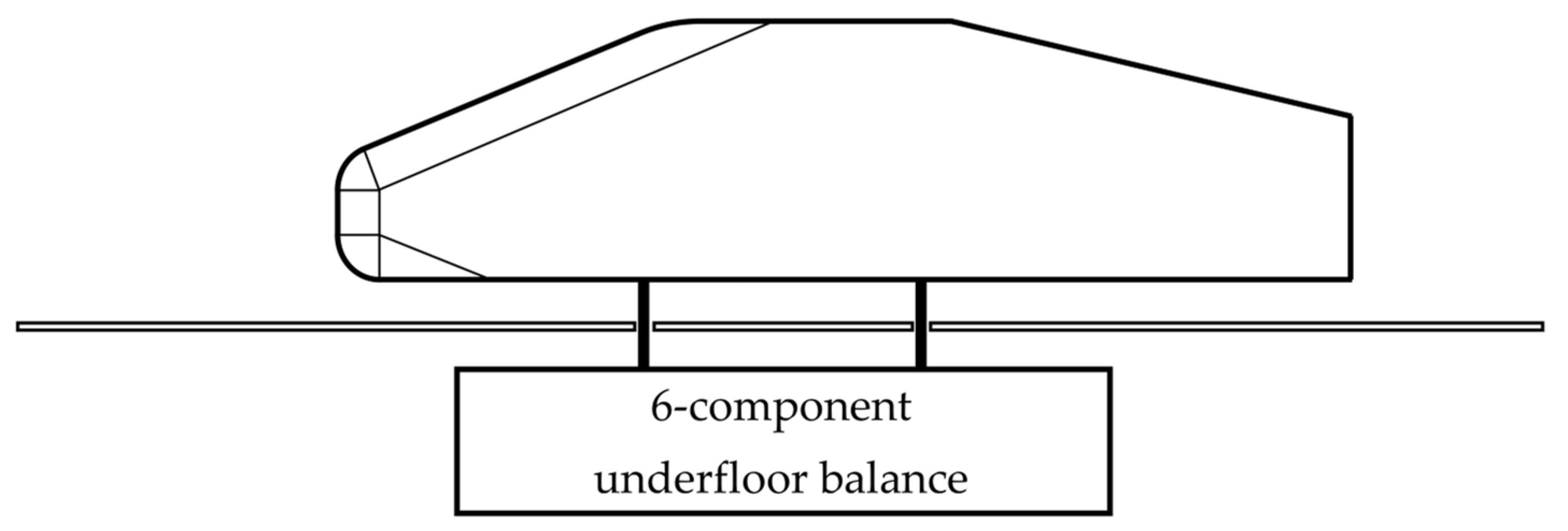
2. Experimental Set-Up
2.1. Model
2.2. Wind Tunnel
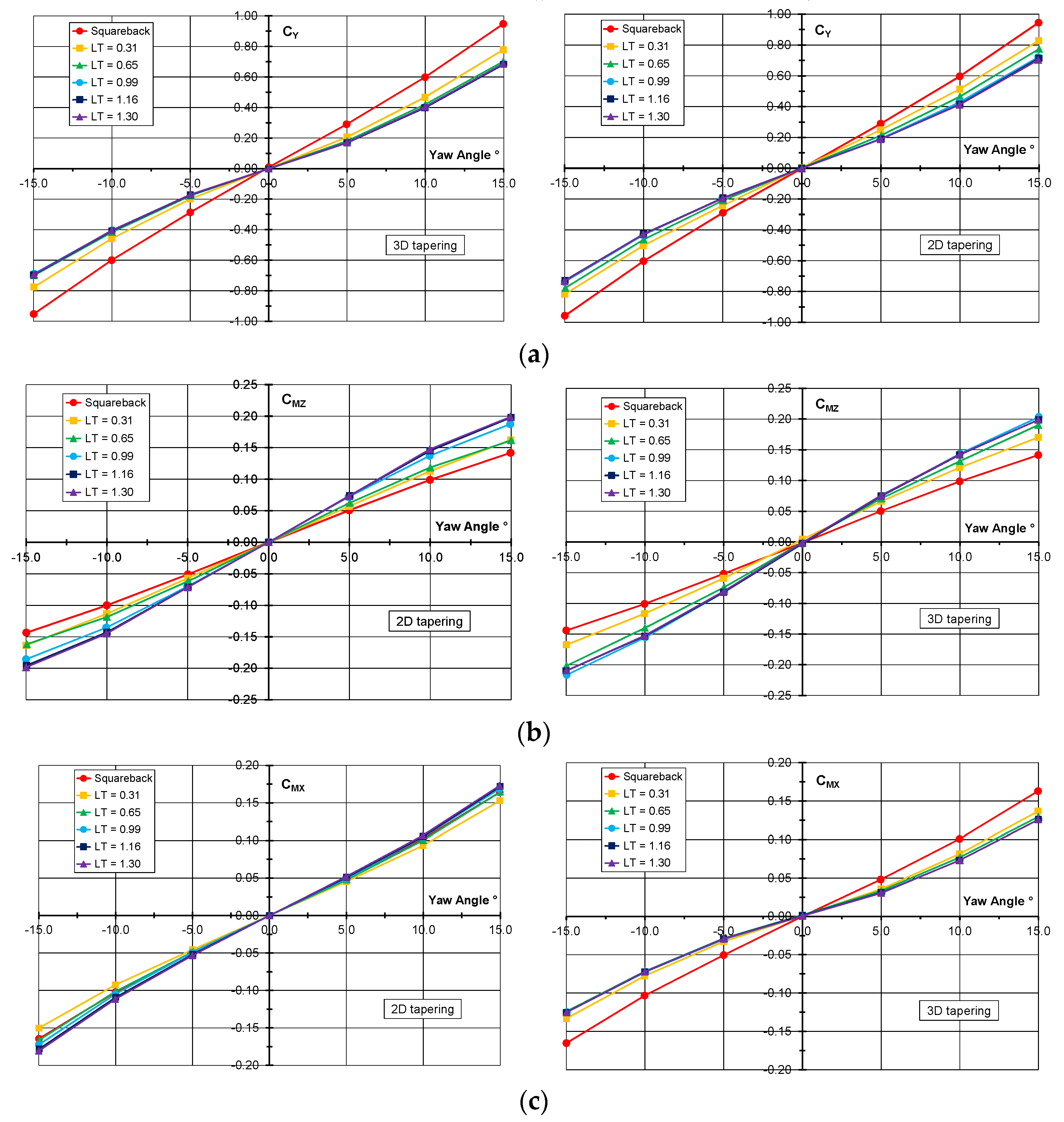
3. Results
4. Discussion
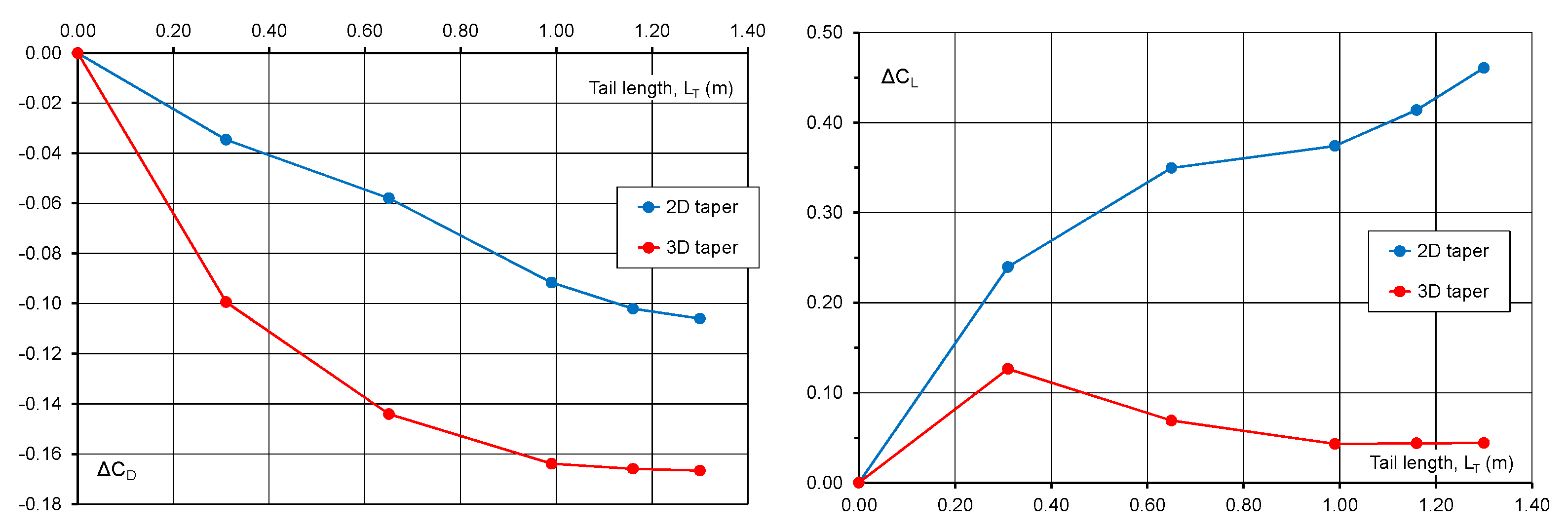
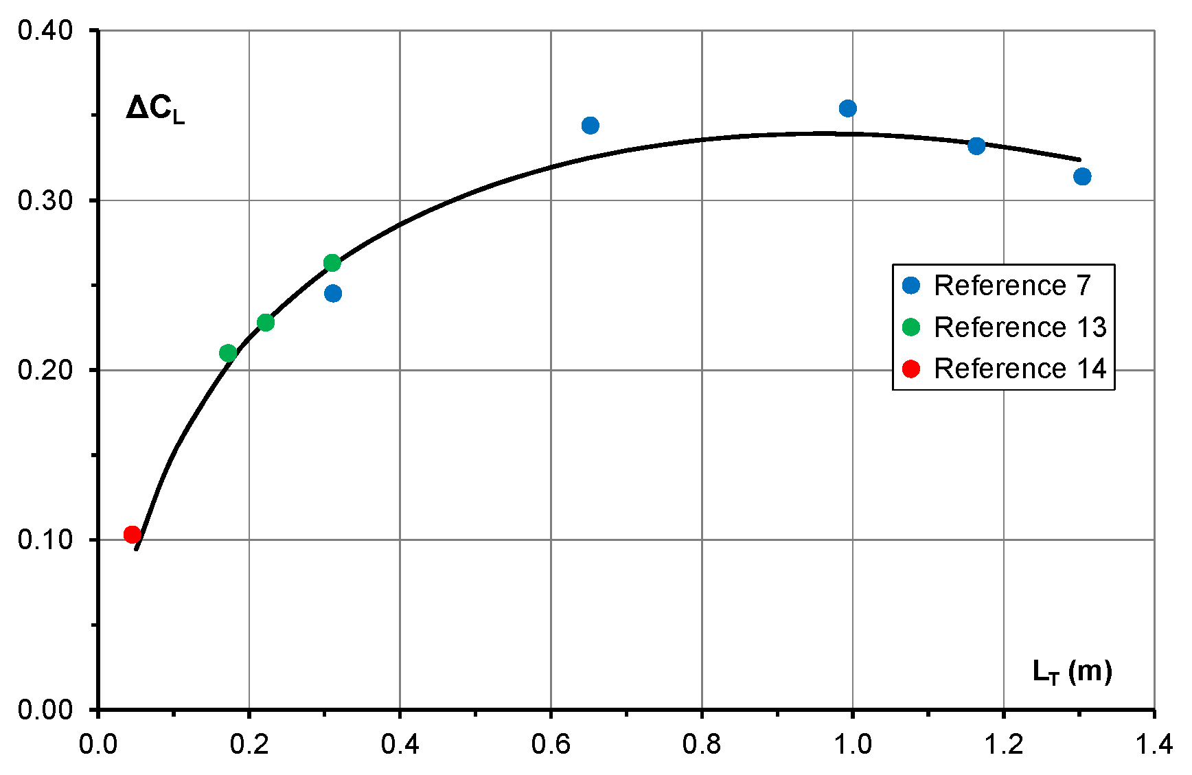
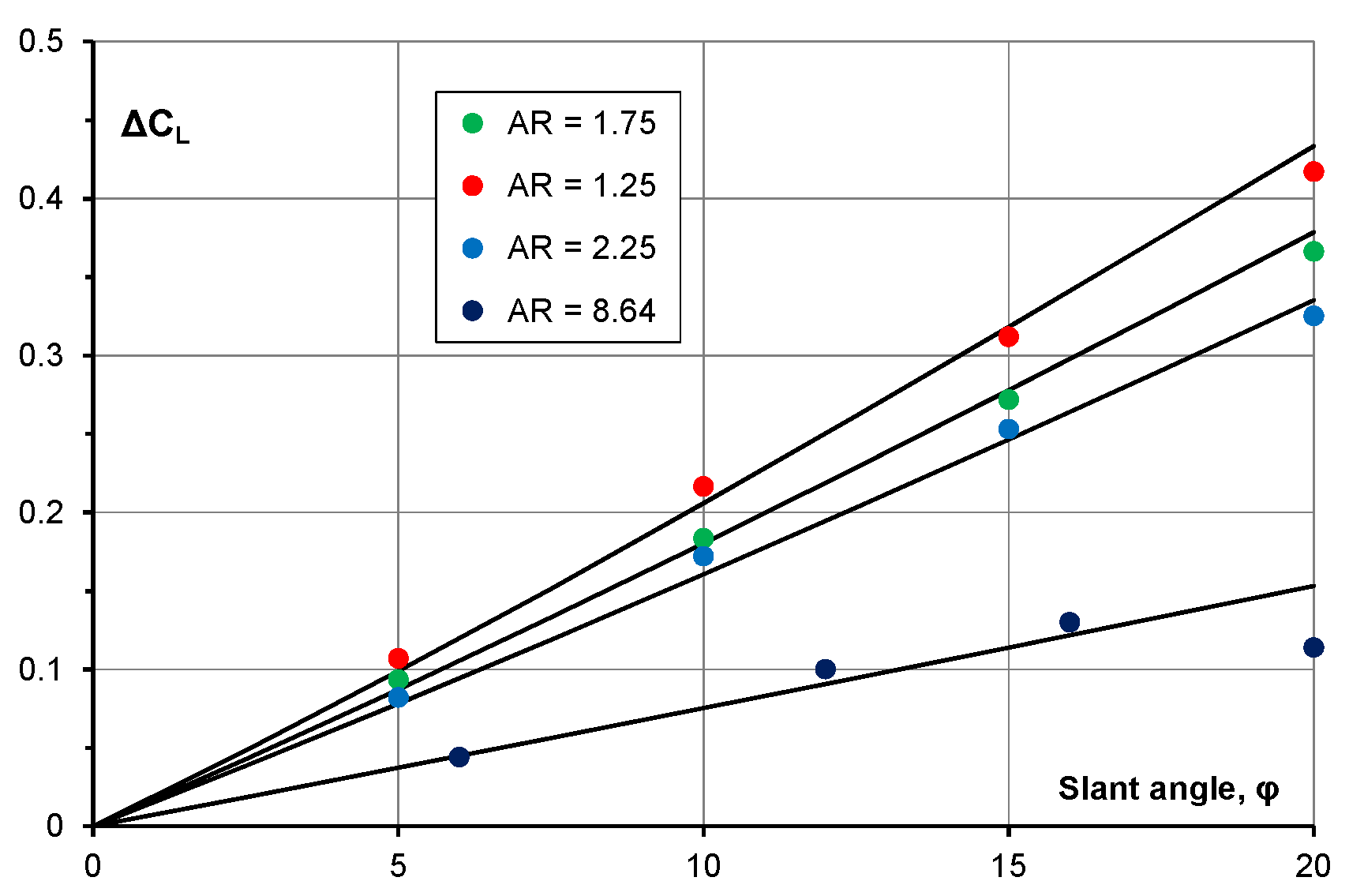
4.1. Effect of Adding Tapered Tails
4.2. Crosswind Sensitivity
4.3. Drag and Lift Breakdown—2D Case
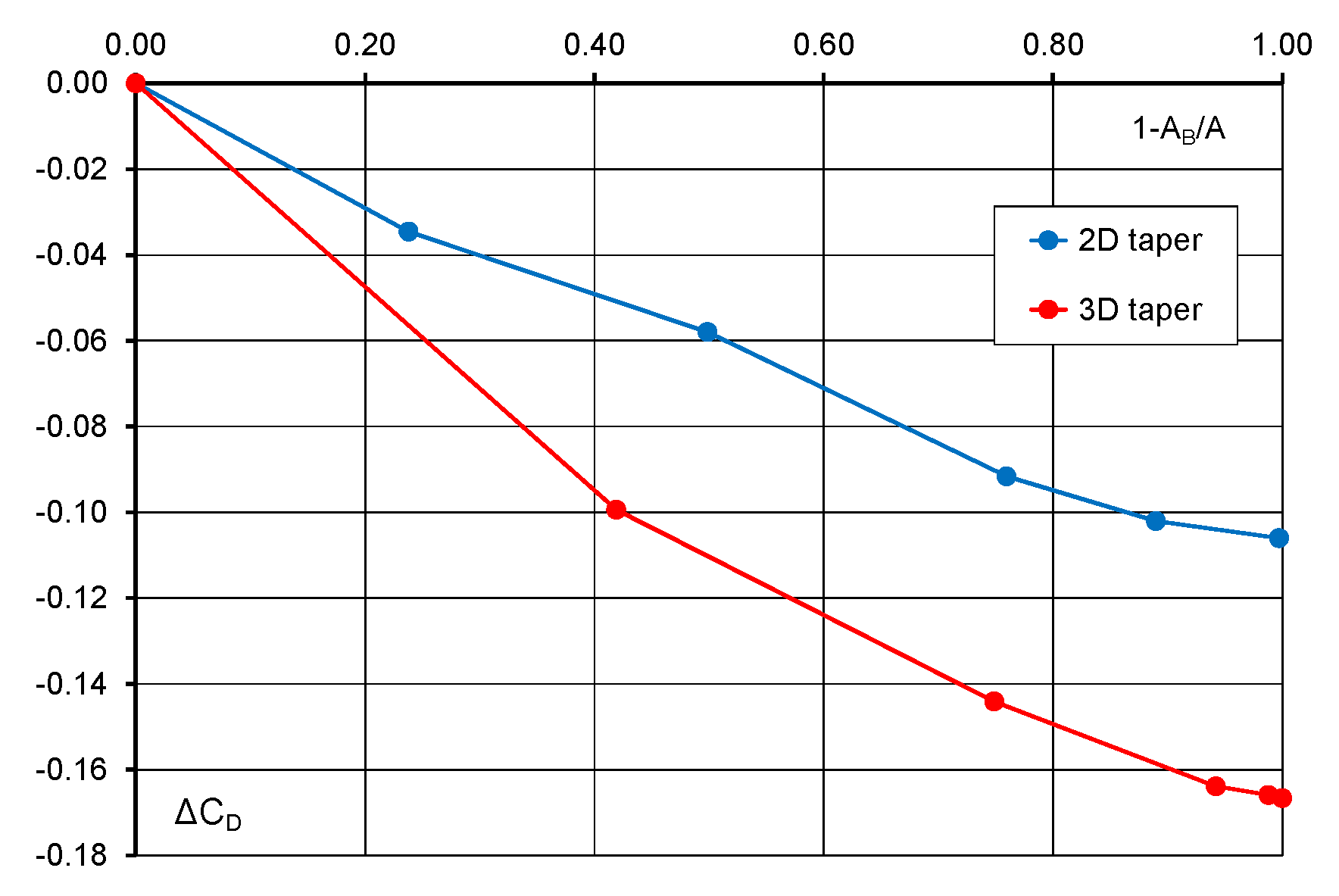
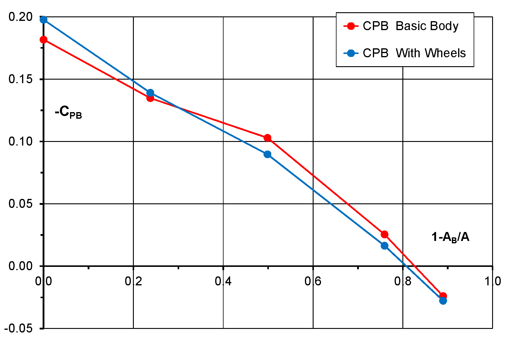
4.4. Base Pressure
4.5. D Tapering
4.6. Final Comments
5. Conclusions
Author Contributions
Funding
Data Availability Statement
Acknowledgments
Conflicts of Interest
Appendix A. A Theory for Lift on a 2D Streamlined Tail


References
- Ludvigsen, K. The Time Tunnel–An Historical Survey of Automobile Aerodynamics; Technical Paper 700035; SAE: Warrendale, PA, USA, 1 February 1970. [Google Scholar] [CrossRef]
- Koenig-Fachsenfeld, R.V. Aerodynamik des Kraftfahrzeuges; Umschau Verlag: Frankfurt, Germany, 1951. [Google Scholar]
- Hucho, W.-H. (Ed.) Aerodynamics of Road Vehicles, 4th ed.; SAE R-177; SAE International: Warrendale, PA, USA, 1998; ISBN 0-7680-0029-7. [Google Scholar]
- Schütz, T. (Ed.) Aerodynamics of Road Vehicles, 5th ed.; SAE R-430; SAE International: Warrendale, PA, USA, 2016; ISBN 978-0-7680-7977-7. [Google Scholar] [CrossRef]
- Edgar, J. A Century of Car Aerodynamics; Amazon, Independently published: London, UK, 2021; ISBN 13 979-8506846901. [Google Scholar]
- Howell, J.; Rajaratnam, E.; Passmore, M. Streamlined Tails–The Effect of Truncation on Aerodynamic Drag; Technical Paper 2020-01-0673; SAE: Warrendale, PA, USA, 14 April 2020. [Google Scholar] [CrossRef]
- Howell, J.; Varney, M.; Rajaratnam, E.; Passmore, M. A Wind Tunnel Study of the Windsor Body with a Streamlined Tail; Technical Paper 2021-01-0954; SAE: Warrendale, PA, USA, 6 April 2021. [Google Scholar] [CrossRef]
- Hoerner, S.F. Fluid Dynamic Drag; Published by the author: Midland Park, NJ, USA, 1958. [Google Scholar]
- Mair, W.A. Reduction of Base Drag by Boat-Tailed Afterbodies in Low-Speed Flow. Aeronaut. Q. 1969, 20, 307–320. [Google Scholar] [CrossRef]
- Johl, G.; Passmore, M.; Render, P. Design Methodology and Performance of an In-Draft Wind Tunnel. Aeronaut. J. 2004, 108, 465–473. [Google Scholar] [CrossRef]
- Howell, J.; Panigrahi, S. Aerodynamic Side Forces on Passenger Cars at Yaw; Technical Paper 2016-01-1620; SAE: Warrendale, PA, USA, 5 April 2016. [Google Scholar] [CrossRef]
- Varney, M. Base Drag Reduction for Squareback Road Vehicles. Ph.D. Thesis, Loughborough University, Loughborough, UK, 2019. [Google Scholar]
- Küchemann, D. The Aerodynamic Design of Aircraft; Pergamom Press: Oxford, UK, 1978; ISBN 0-08-020515-1. [Google Scholar]
- Howell, J.; Le Good, G. The Effect of Backlight Aspect Ratio on Vortex and Base Drag for a Simple Car-like Shape; Technical Paper 2008-01-0737; SAE: Warrendale, PA, USA, 14 April 2008. [Google Scholar] [CrossRef]
- Pavia, G. Characterisation of the Unsteady Wake of a Square-Back Vehicle. Ph.D. Thesis, Loughborough University, Loughborough, UK, 2019. [Google Scholar]


Disclaimer/Publisher’s Note: The statements, opinions and data contained in all publications are solely those of the individual author(s) and contributor(s) and not of MDPI and/or the editor(s). MDPI and/or the editor(s) disclaim responsibility for any injury to people or property resulting from any ideas, methods, instructions or products referred to in the content. |
© 2023 by the authors. Licensee MDPI, Basel, Switzerland. This article is an open access article distributed under the terms and conditions of the Creative Commons Attribution (CC BY) license (https://creativecommons.org/licenses/by/4.0/).
Share and Cite
Howell, J.; Varney, M.; Passmore, M.; Butcher, D. The Aerodynamic Effects of a 3D Streamlined Tail on the Windsor Body. Fluids 2023, 8, 59. https://doi.org/10.3390/fluids8020059
Howell J, Varney M, Passmore M, Butcher D. The Aerodynamic Effects of a 3D Streamlined Tail on the Windsor Body. Fluids. 2023; 8(2):59. https://doi.org/10.3390/fluids8020059
Chicago/Turabian StyleHowell, Jeff, Max Varney, Martin Passmore, and Daniel Butcher. 2023. "The Aerodynamic Effects of a 3D Streamlined Tail on the Windsor Body" Fluids 8, no. 2: 59. https://doi.org/10.3390/fluids8020059