Article

A New Rheological Model for Phosphate Slurry Flows

by
Zeineb Ghoudi
1,2,
Souhail Maazioui
3,
Fayssal Benkhaldoun
2,* and
Noureddine Hajjaji
1
1
Laboratoire de Recherche Catalyse et Materiaux pour l’Environnement et les Procedes LRCMEP (LR19ES08), Ecole Nationale d’Ingenieurs de Gabes, Universite de Gabes, Rue Omar Ibn Alkhattab, Gabes 6029, Tunisia
2
LAGA, Sorbonne Paris Cité, Université Sorbonne Paris Nord, UMR 7539 Villetaneuse, France
3
Modeling Simulation & Data Analysis (MSDA), Mohammed VI Polytechnic University, Lot 660-Hay Moulay Rachid, Benguerir 43150, Morocco
*
Author to whom correspondence should be addressed.
Fluids 2023, 8(2), 57; https://doi.org/10.3390/fluids8020057
Submission received: 9 December 2022 / Revised: 20 January 2023 / Accepted: 27 January 2023 / Published: 8 February 2023
(This article belongs to the Special Issue Advances in Computational Mechanics of Non-Newtonian Fluids)

Abstract

:
In this paper, a new rheological model for the flow of phosphate-water suspensions is proposed. The model’s ability to replicate the rheological characteristics of phosphate-water suspensions under different shear rate conditions is evaluated using rheometric tests, and it is found to be in good agreement with experimental data. A comprehensive methodology for obtaining the model parameters is presented. The proposed model is then incorporated into the OpenFoam numerical code. The results demonstrate that the model is capable of reproducing the rheological behavior of phosphate suspensions at both low and high concentrations by comparing it with suitable models for modeling the rheological behavior of phosphate suspensions. The proposed model can be applied to simulate and monitor phosphate slurry flows in industrial applications.

1. Introduction

Numerical modeling of multiphase flows along with complex rheology has particularly drew considerable attention during the last two decades and the study of their behavior has led to a large literature. Such complex phenomena are encountered in many industrial and engineering applications, including evaporation and condensation [1], flooding events [2,3], chemical and nuclear reactors [4], fluidized bed [5], combustion and fuel atomization [6,7]. Recently, researchers have devoted a considerable amount of research efforts into developing and implementing sophisticated mathematical techniques, relevant in the whole range of multi-fluid and multiphase flow problems. Being the two main families of solution methods, Level-Set (LS) and Volume-Of-Fluid (VOF) proposed respectively by Sussman et al. [8] and Hirt et al. [9] are the two most commonly employed approaches which have assisted in better understanding of the underlying physics governing the multiphase flows in different fields. Given the particularities of each model, VOF and LS have been widely used to investigate a broad range of engineering problems such as Rayleigh–Taylor Instability [10], dam failure phenomena [11,12,13], bubble rising/nucleation [14,15,16], droplet impact on both dry and wet surfaces [17,18,19,20], metallurgical engineering [21], to mention only a few. In this study, we use the VOF method to investigate water-slurry modeling in a horizontal pipeline.
Viscoplastic or yield-stress fluids are materials which behave as solids as the shear rate tends to zero, and as liquids beyond a certain critical shear stress level ( τ 0 ) . In particular, simple yield-stress fluids are materials that are both non-thixotropic and inelastic, and characterized by a shear stress that depends only on the applied shear rate, and materials [22]. The most popular simple viscoplastic model was first proposed by Bingham [23] and is defined by a yield stress value and a constant plastic viscosity representing the slope of the shear stress versus shear rate curve. The Bingham constitutive equation can be expressed as follows:
γ ˙ = 0 if   | τ | τ 0 τ = μ + τ 0 | γ ˙ | γ ˙ if   | τ | > τ 0
where τ and γ ˙ are the stress tensor and the shear rate tensor respectively. While the terms τ 0 , and μ indicate the yield stress and the plastic viscosity scalar values. | τ | = 1 2 τ : τ and | γ ˙ | = 1 2 γ ˙ : γ ˙ denote the second invariants of τ and γ ˙ , respectively. The strain rate tensor γ ˙ is defined as γ ˙ = u + ( u ) T , u being the velocity vector. The flow domain of a yield stress fluid is divided into a yielded region ( | τ | > τ 0 ) and an unyielded ( | τ | τ 0 ) region, separated by the yield surfaces where | τ | = τ 0 . Two well known generalizations of the Bingham fluid model have been proposed by Herschel–Bulkley [24], and Casson [25], formulated respectively as:
Herschel-Bulkley : τ = K | γ ˙ | ( n 1 ) + τ 0 | γ ˙ | γ ˙ if   | τ | > τ 0
Casson : τ = μ | γ ˙ | + τ 0 2 γ ˙ | γ ˙ | if   | τ | > τ 0
where K is the consistency and n is the power-law index. The flexibility of the Herschel–Bulkley model to fitting various experimental data makes it very popular among other yield stress models. Moreover, the Herschel–Bulkley model can be reduced to power-law and Casson models when setting the yield stress to zero τ 0 = and the power-law index to n = 1 , respectively. According to [26], the power law, the Bingham plastic, the Casson and the Herschel–Bulkley models remain the four widely used models for describing the viscous properties of suspensions.
Various research works have studied slurry flows as a continuum non-Newtonian fluid based on the equivalence assumption and have made use of either Bingham model or Herschel–Bulkley (H–B) model to represent the rheological properties [27,28]. Hamza et al. (2018) [29] have investigated in their work the rheological behavior of the phosphate-water slurry in an attempt to determine a model capable of describing its flow behavior. They came to the conclusion that the Herschel–Bulkley model is a suitable model for representing the rheological behavior of the phosphate slurry for low concentrations (less than 38.45 wt%). For higher concentrations in the range of 34.24–46.03 wt%, the Bingham model was more adequat. Finally, the Casson model was the best fitting model for calculating viscosity and yield stress for the range of concentrations (46.03–57.27 wt%). In addition, based on the experimental results, they conclude that the phosphate slurry rheological behavior tends to be a dilatant behavior beyond a concentration of 38.45 wt%.
The aim of this work is to develop a model that could describe the rheological behavior of the phosphate slurry over a wide range of concentrations. We will show that the model is capable of reproducing the rheological behavior that phosphate suspensions may exhibit in both low and high concentrations. This is achieved by comparing the output of the model with those of the models suitable for modeling the rheological behavior of phosphate slurry. A methodology for obtaining the model’s parameters is presented in details. Whilst the term “multi-phase flows” covers the whole spectrum of gas–liquid, liquid–liquid, gas–solid, liquid–solid, gas–liquid–solid and gas–liquid–liquid systems, our concern in this work is to investigate the simultaneous co-current flow of a simple liquid and a non-Newtonian suspension of solid particles. The new model presented in this paper should be of interest to broad and diverse areas of application. Furthermore, the subject may be relevant both to theoretical mathematicians and practising engineers with a wide range of backgrounds.

2. Materials and Methods

The flow behavior of the materials encountered in many chemical and process engineering applications is highly influenced by the characteristics of their components, including their non-Newtonian properties, shape, size and concentration of the suspended particulates, the applied shear rate and the geometry of the system. In general, the flow behavior of such systems is so complex that theoretical treatments, which tend to apply to highly idealized problems, have proved to be of little practical utility. Therefore, flow investigations rely heavily on analyses of the behavior of such systems in practice based on experimental work and well established assumptions.

2.1. The New Rheological Model

Over the years, to model the stress-deformation behavior, several empirical expressions have been proposed as a result of straightforward curve-fitting exercises and different yield criteria have been used. The majority of the available literature is empirical and still need to be developed, partially due to the difficulty of obtaining accurate, reliable data on yield stress materials over a wide range of shear rates.
In this paper, we seek to investigate the rheological behavior of the Phosphate slurry, which is a mixture of insoluble particles and a continuous phase of water. The obtained rheograms of this material show a non-Newtonian flow behavior exhibiting a yield stress as the shear rate tends to zero. A two-branch model equation is presented to embrace the non-linear flow of phosphate slurry over a very large range of shear rates. In one dimensional steady shearing motion, it is written as:
τ = a ( γ ˙ + γ ˙ 0 ) b if   γ ˙ < γ ˙ c τ c + γ ˙ η if   γ ˙ c γ ˙
where the parameters a and b can be considered similar to the the consistency and the power-law index of the Herschel–Bulkley model, respectively. On the other hand, the parameter γ ˙ 0 has a different interpretation than the model parameters of both Herschel–Bulkley or Bingham model. In this model, γ ˙ 0 can be regarded as a correction to the shear rate rather than the shear stress and the yield stress is defined as τ y = a γ ˙ 0 b . The linear part of the curve is described using the parameters η and τ c , which represent respectively the consistency index [Pa·s], the yield stress [Pa]. The transition from one branch to the other depends on the critical value of shear rate which is experimentally defined as γ ˙ c = 400 s 1 in the particular case of phosphate slurries considered in this work.
To determine the rheological coefficients of each model equation, we perform a curve fitting based on the least square method. Curved relationships between variables are not as straightforward to fit and interpret as linear relationships. Given M data pairs ( γ ˙ m , τ m ) where m { 1 , . . . , M } , the parameters of Equation (4) need to be determined. We consider the general case where the model can be formulated as τ = f ( θ , γ ˙ ) where θ is a vector of p parameters. In what follows, the least squares approach is applied to determine the parameters which to minimise the following expression:
m i n θ m = 1 M [ τ m f ( θ , γ ˙ m ) ] 2
where the pairs ( γ ˙ m , τ m ) are observed. Given the observed data pairs { ( γ ˙ 1 , τ 1 ) , , ( γ ˙ M , τ M ) } , we may define the error associated to the second branch of Equation (4), τ = τ c + γ ˙ η , by:
E ( η , τ c ) = m = 1 M ( τ m ( τ c + γ ˙ m η ) ) 2
Our goal is to define the values of η and τ c that minimize the error function. Following the least-squares method, we should find the values of ( η , τ c ) such that:
E η = 0 , E τ c = 0
It is to be noted that, in this case, we do not have to worry about boundary points: as | η | and | τ c | become large, the fit will clearly deteriorate. Thus we do not need to check on the boundary. Differentiating E ( η , τ c ) yields:
E η = m = 1 M 2 ( τ m ( τ c + γ ˙ m η ) ) ( γ ˙ m )
E τ c = m = 1 M 2 ( τ m ( τ c + γ ˙ m η ) )
Setting E / η = E / τ c = 0 and dividing by 2 yields:
m = 1 M ( τ m ( τ c + γ ˙ m η ) ) γ ˙ m = 0
m = 1 M ( τ m ( τ c + γ ˙ m η ) ) = 0
We may rewrite these equations as:
m = 1 M γ ˙ m 2 η + m = 1 M γ ˙ m τ c = m = 1 M τ m γ ˙ m
m = 1 M γ ˙ m η + m = 1 M 1 τ c = m = 1 M τ m
We have obtained that the values of η and τ c which minimize the error (defined in Equation (6)) satisfy the following matrix equation:
m = 1 M γ ˙ m 2 m = 1 M γ ˙ m m = 1 M γ ˙ m m = 1 M 1 η τ c = m = 1 M τ m γ ˙ m m = 1 M τ m
We will show the matrix is invertible, which implies
η τ c = m = 1 M γ ˙ m 2 m = 1 M γ ˙ m m = 1 M γ ˙ m m = 1 M 1 1 m = 1 M τ m γ ˙ m m = 1 M τ m
We denote the matrix by A. The determinant of A is
d e t A = m = 1 M γ ˙ m 2 . m = 1 M 1 m = 1 M γ ˙ m . m = 1 M γ ˙ m
As
γ ˙ m ¯ = 1 M m = 1 M γ ˙ m
we find that,
d e t A = M m = 1 M γ ˙ m 2 ( M γ ˙ m ¯ ) 2 = M 2 1 M m = 1 M γ ˙ m 2 γ ˙ m ¯ 2
where the last equality is derived from simple algebra. Hence, while γ ˙ m are not all equal, d e t A will be nonzero and A will be invertible. Therefore, we note that as long as γ ˙ m are not all equal, the best-fit values of η and τ c are achieved by solving a system of linear equations in the Equation (15). As for the first branch of Equation (4), it requires an initial estimate for one of the three parameters. We can use the following procedure for the estimation of these parameters. γ ˙ 0 can be estimated first using the following equation:
γ ˙ 0 = γ ˙ m i n γ ˙ m a x γ ˙ * 2 2 γ ˙ * γ ˙ m i n γ ˙ m a x
where γ ˙ * is the shear rate corresponding to the geometric mean of the maximum and minimum shear stresses:
τ * = ( τ m i n τ m a x ) 1 / 2
Then, taking the logarithm of the first branch of Equation (4):
log ( τ ) = log ( a ) + b log ( γ ˙ + γ 0 ˙ )
and using the same methodology described above, one can obtains the two remaining parameters by change of variables then calculation.
The proposed model, which is based on the formulation described earlier, has been implemented using the OpenFoam numerical code. This powerful open-source framework offers a wide range of options for modeling the behavior of fluids, including a library of viscosity models such as Bingham, Herschel–Bulkley, and Casson. These models are defined in terms of strain rate and can be easily customized by the user to suit the specific requirements of their application. Additionally, the transportProperties dictionary allows for further flexibility in defining the rheological properties of the fluids being modeled. The implementation of the proposed model using the OpenFoam framework thus enables a more accurate and comprehensive simulation of multiphase flows and complex rheology in various industrial and engineering applications.

2.2. Numerical Modelling

The new model is applied to multiphase flow to account for the true behavior of phosphate slurry and its deformations that occur during this engineering instance. The simplest way to solve a two-fluid flow is to track the interface between the two fluid phases with a simple α indicator, often referred to in the literature as a concentration function. This method is called VOF (Volume-Of-Fluid) method, other approaches include Level-Set, Front Tracking, etc. twoLiquidMixingFoam [30,31] is a well-established solver for the simulation of flows in which two incompressible fluids are present. A separate surface interface can be defined based on the VOF method in OpenFOAM, which is a free and open-source parallel processing software supported by a large user community [27,32]. The different phases are represented in the domain by their phase fractions using the VOF [9,33]. This method allows to reduce considerably the computational costs.
An algebraic VOF method is used in the twoLiquidMixingFoam solver, which is a modified version of the VOF method of Hirt and Nichols (1981) [9] by adding a diffusion term. The phosphate slurry consists of solid particles and water. In this paper, we considered the homogenenous regime of the slurry with constant density and viscosity across the pipe. Therefore the two-phase system is the slurry phase and the water batch.

2.2.1. Governing Equations

The sum of the volume fractions of all phases in a cell is equal to unity and is given by the Equation (22) below
α s + α w = 1
where α s and α w denote the volume fraction of the slurry and water phases respectively. Both phases are assumed to be incompressible. The continuity equation is given as follows
· v = 0
where v represent the velocity. The momentum equation solved for both the phases during the simulation is given by equation
ρ v t + ρ v ( · v ) = P + · τ + ρ g + F c s
where P and g are the pressure and acceleration due to gravity, respectively. τ represents the shear stress tensor; for Newtonian fluids, it is a linear function of the shear rate given by
τ = μ γ ˙ = μ v + ( v ) T 2 3 · v I
where μ is the dynamic viscosity of the Newtonian fluid. For non-Newtonian materials, a different relation is available in which μ a p is the apparent viscosity of the non-Newtonian fluid
τ = μ a p γ ˙
Several rheological models have been developed in the literature to describe the behaviour of these materials. In this work, the models used to describe the behaviour of the phosphate slurry are Herschel-Bulkley (Equation (2)), Casson (Equation (3)) and the proposed model (Equation (4)).
F c s represents the surface tension force which is modeled as a volumetric force by the continuum surface force (CSF) model of Brackbill et al. [34]. For two-phase system, the value of F c s is expressed by Equation (27)
F c s = σ ρ k α s 0.5 ( ρ w + ρ s )
where σ represents the surface tension coefficient and k the interface curvature, which is further expressed by Equations (28) and (29) respectively
k = · n ^
n ^ = α s | α s |
The interface between the two phases progresses thanks to the volume fraction Equation (30)
α s t + · ( v α s ) = · ( Γ t α s )
Γ t = D A B + ν t S c t
where α s is the cell fraction of the slurry phase, Γ t is the effective diffusivity, D A B represents the coefficient of molecular diffusion, ν t is the turbulent viscosity, and S c t denotes the turbulent Schmidt number. The coefficient of diffusion D A B and the turbulent Schmidt number S c t were set to 1.0 × 10 6 m 2 /s and 1.0 , respectively. The phase fraction in a cell is related to the RANS model by density as follows
ρ = α s ρ s + α w ρ w = α s ρ s + ( 1 α s ) ρ w
where ρ s represents the density of the slurry that corresponds to the α s phase fraction, while ρ w is the density that corresponds to the water phase with the α w phase fraction. The calculated density ρ in the Equation (32) should not be considered as a real density of the fluid but as a density of the phase mixture that occupies a cell in the finite volume framework. The RANS model uses the density ρ in the conservation of momentum equation. When α s is equal to 1, the represented phase is the slurry while the water phase α w is defined as 0, and vice versa. Any value between 1 and 0 describes a mixture and can also be interpreted as a percentage of the amount of this or that fluid present in a cell. The Equation (30) can be interpreted as an advection–diffusion equation for the α s phase.

2.2.2. Turbulence Equations

However, we should mention that all the constants and wall function of the k ω S S T model have been derived experimentally by measurements on Newtonian fluids [35]. Moreover, they are not adapted to non–Newtonian fluids. In the present work, we have used k ω S S T model to simulate the flow of water pushing the slurry batch, thus the turbulence is applied to the water batch.
The transport equations of the turbulent kinetic energy k and the specific dissipation rate ω are
k t + ( k v i ) z i = 1 ρ z j Γ k k z j + G ˜ k Y k + S k
ω t + ( ω v i ) z i = 1 ρ z j Γ k ω ω z j + G ˜ ω + Y ω + D ω + S ω
where G ˜ k is the generation of turbulence kinetic energy due to the mean velocity gradients. G ˜ ω denotes the generation of the specific dissipation rate. Γ k and Γ ω are the effective diffusivity of k and ω respectively. Y k and Y ω represent the dissipation of k and ω due to turbulence. D ω is the cross-diffusion term. S k and S ω represent source terms set to be zero in this study. All the above terms are calculated and specified in [36,37,38,39].

3. Results and Discussions

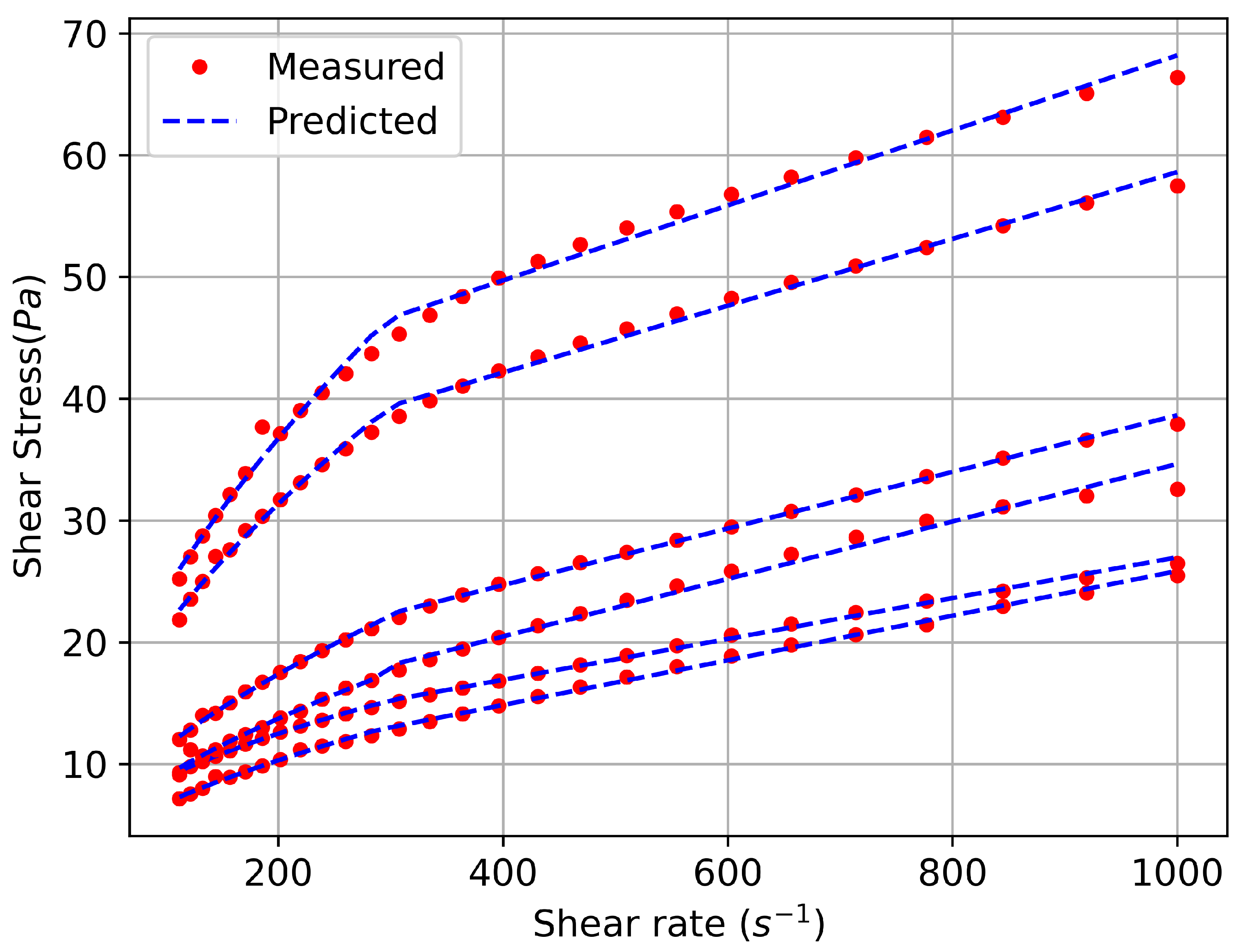
3.1. Rheological Evaluation of the New Model

In the present study, we used phosphate ore samples of different grades and concentrations of 51, 54, and 56 wt% in water. These samples were labeled S1 to S6 and different primarily in their solids concentrations. The details on the rheological data and samples characteristics can be found in [40]. The rheograms of phosphate slurries were obtained, at room temperature, by applying a ramp of predefined shear rate decreasing from 1000 s 1 to 112 s 1 , and measuring the corresponding shear stress. The diameters of the rotating bob and the cylindrical cup are respectively 38.713 mm and 44 mm. Prior to each measurement, the suspensions were stirred carefully in a vessel to wipe out material memory and obtain the same initial conditions for both samples and then rapidly filled into the external cylinder. The effects of wall slip were not completely prevented using this geometry, so any reproduction of the resulting rheograms should be carried out with caution. The experimental data are shown in Figure 1.
The accuracy of the New model is checked by fitting the phosphate slurry data. Figure 1 shows a good agreement with the experimental data for six samples of the phosphate slurry.

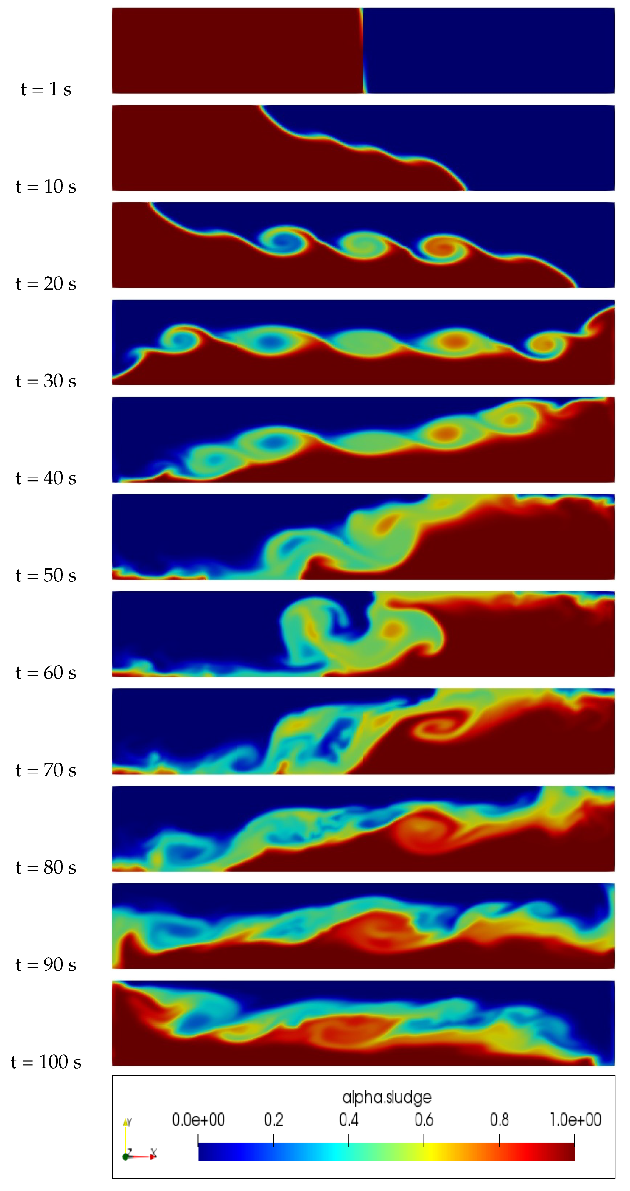
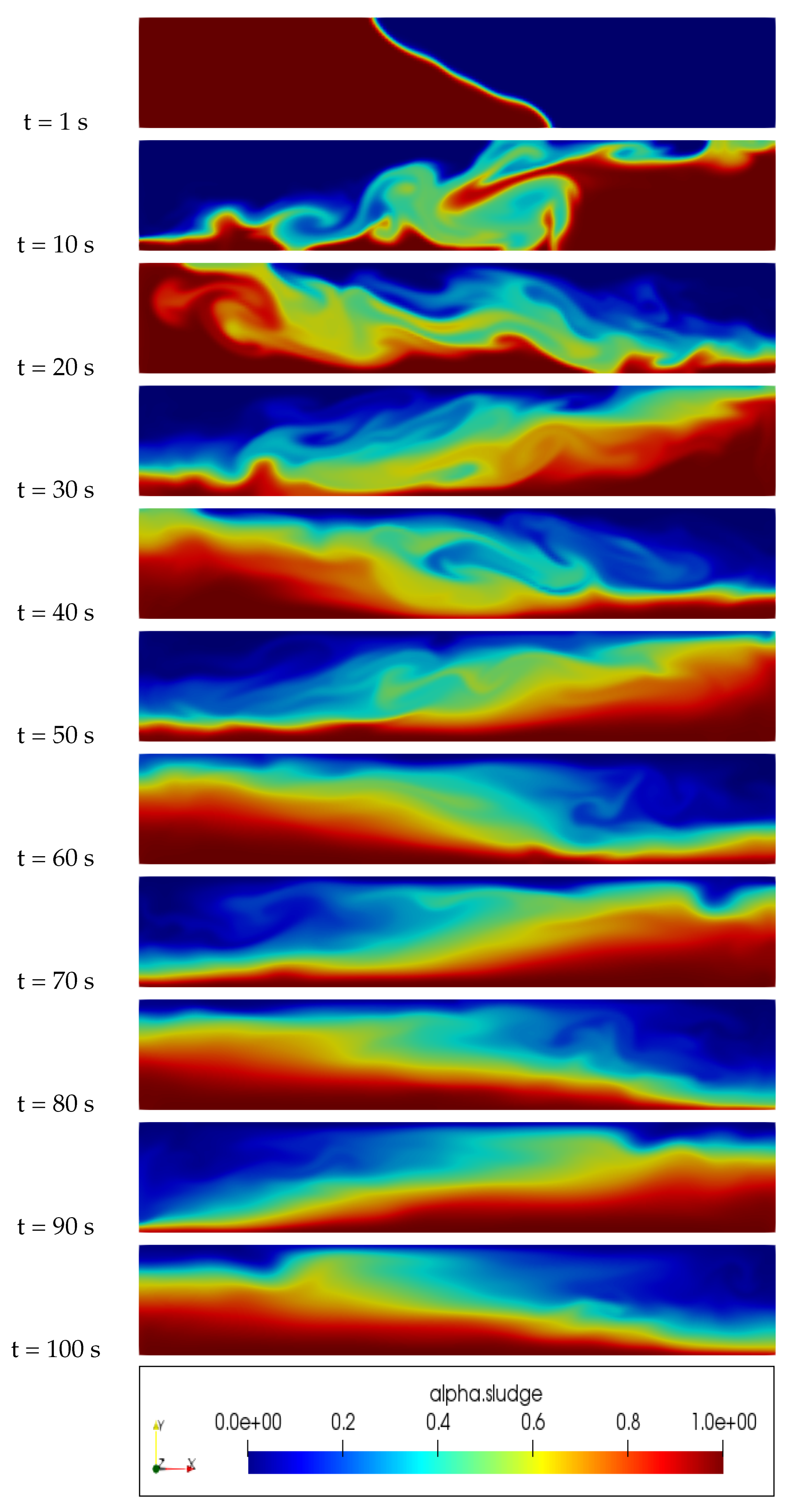
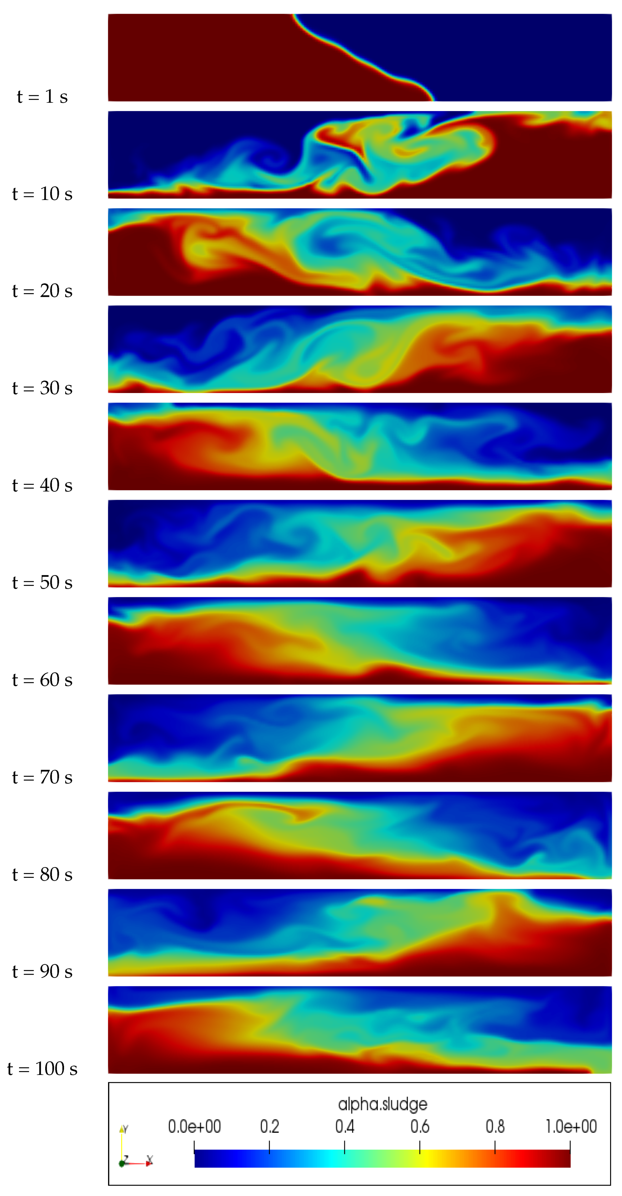
3.2. Numerical Results

OpenFoam 9.0, the open source CFD framework was used to solve the flow equations, turbulence models and transport equations. It is a very flexible CFD code where each component can be personalized to meet the user’s needs. In single-phase flow calculations, the SIMPLE algorithm is used to couple pressure with velocity, whereas the PIMPLE algorithm is used in bi-phase simulations. In the single-phase simulations, the relaxation factors used are 0.5 for U, k and ϵ and 0.3 for the pressure. While, in the two-phase flow case, the relaxation factor for all variables is 1. GAMG is the linear solver used for pressure, and the smooth solver was adopted for U, k, ϵ and α .

3.2.1. Model Implementation

The new model is implemented in the OpenFoam 9.0 source code. The test case “lock-Exchange”, implemented in OpenFoam library, is used to test the new model. Since performing numerical simulations of a yield stress material flow is not a straightforward task, the regularization method was widely used in the last decades, see [41,42] and references therein. The regularization approach includes methods which approximate viscosity value by one regularized and smooth constitutive equation, which is well determined regardless of the shear rate magnitude. The regularized equation treats the whole material domain as a fluid of variable viscosity and locally assigns a large but finite value of viscosity to the unyielded regions. Similary, In OpenFoam, the material is modelled for low strain rates as a very viscous fluid with a high viscosity μ 0 defined by the user. Beyond a threshold in strain-rate corresponding to threshold stress, the viscosity is described by a the constitutive equations. Thus the implementation is formulated as: μ = m i n ( μ 0 , μ ( γ ˙ ) ) . The physical characteristics of the two phases used water and sludge are represented in Table 1. The multiphase solver used twoLiquidMixingFoam is described in Table 2.
For the purpose of comparison, three rheological models already present in the OpenFOAM library were employed—the Newtonian, Casson, and Herschel–Bulkley models. The S1 pulp sample was used in this comparison, with the values defined in Table 3 being assigned to the variables ‘a’ and ‘b’ respectively.
An examination of Figure 2, Figure 3, Figure 4 and Figure 5 reveals significant differences in the distribution of sludge concentration within the column when using the proposed new model in comparison to other models such as the Newtonian, Casson, and Herschel–Bulkley models. While the latter models tend to result in the mixing and formation of eddies between the water and sludge, the new model maintains a clear physical interface between the two fluids. This prevents mixing over time and instead results in a clear layering of the denser sludge at the bottom of the pipe and the less dense water at the top. This behavior can be clearly observed in the figures and highlights the potential advantages and unique properties of the new model in the simulation of multiphase flows and complex rheology in various industrial and engineering applications.

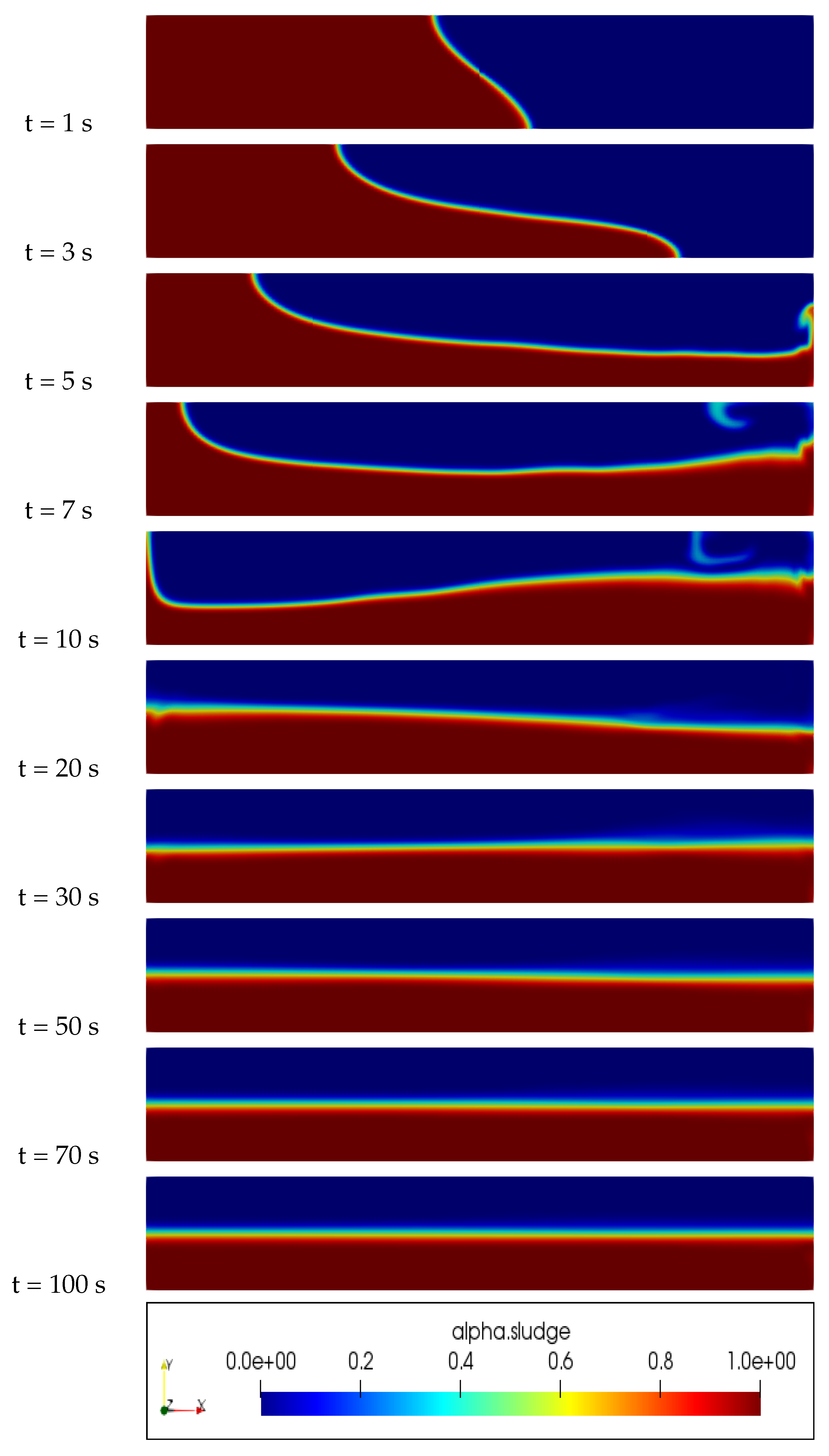
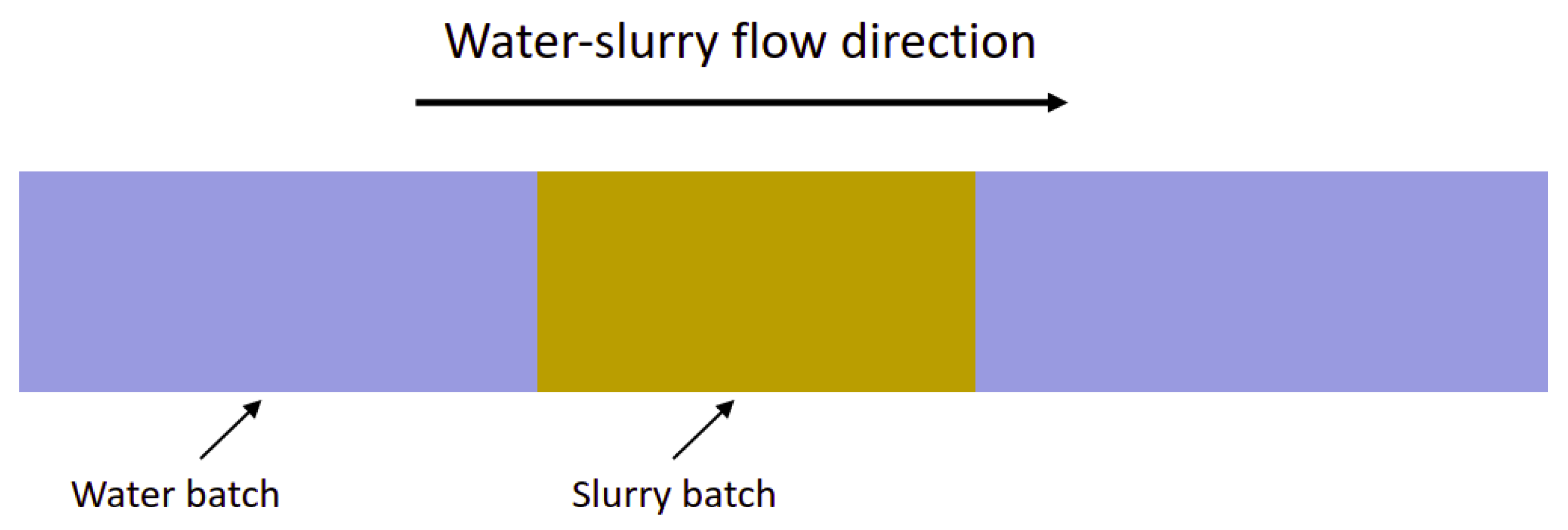
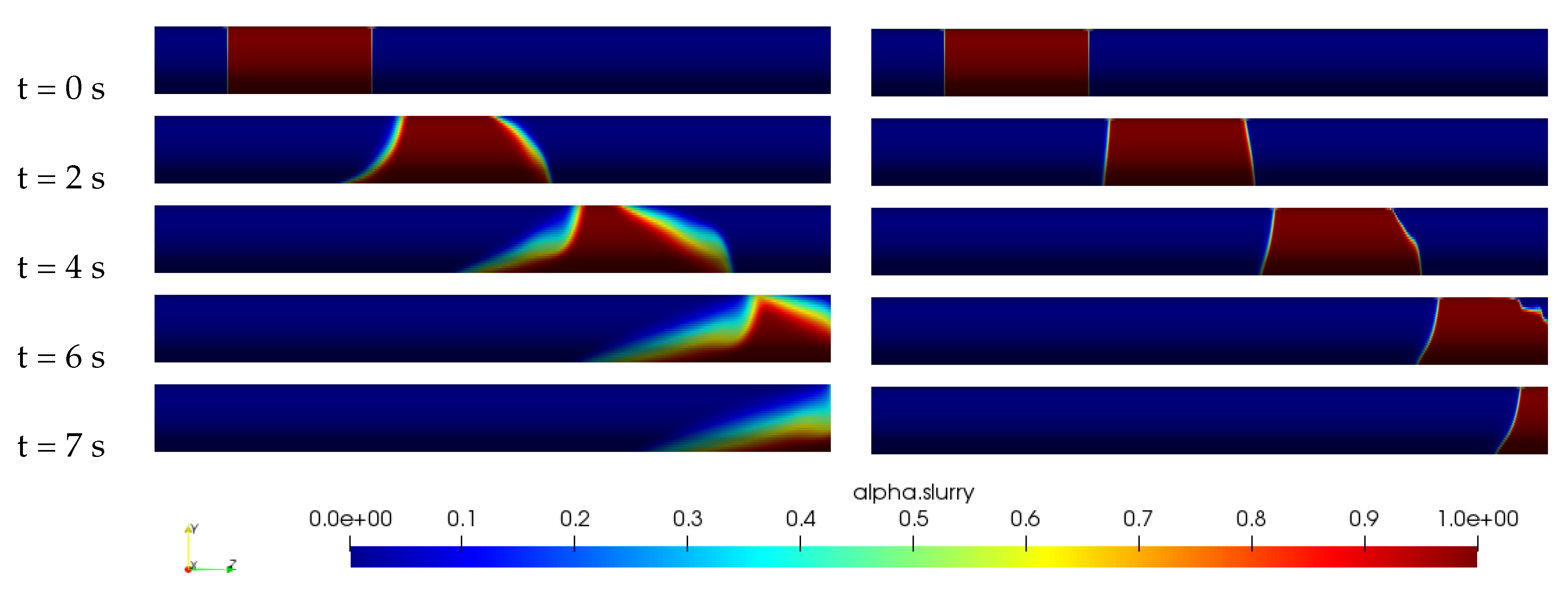
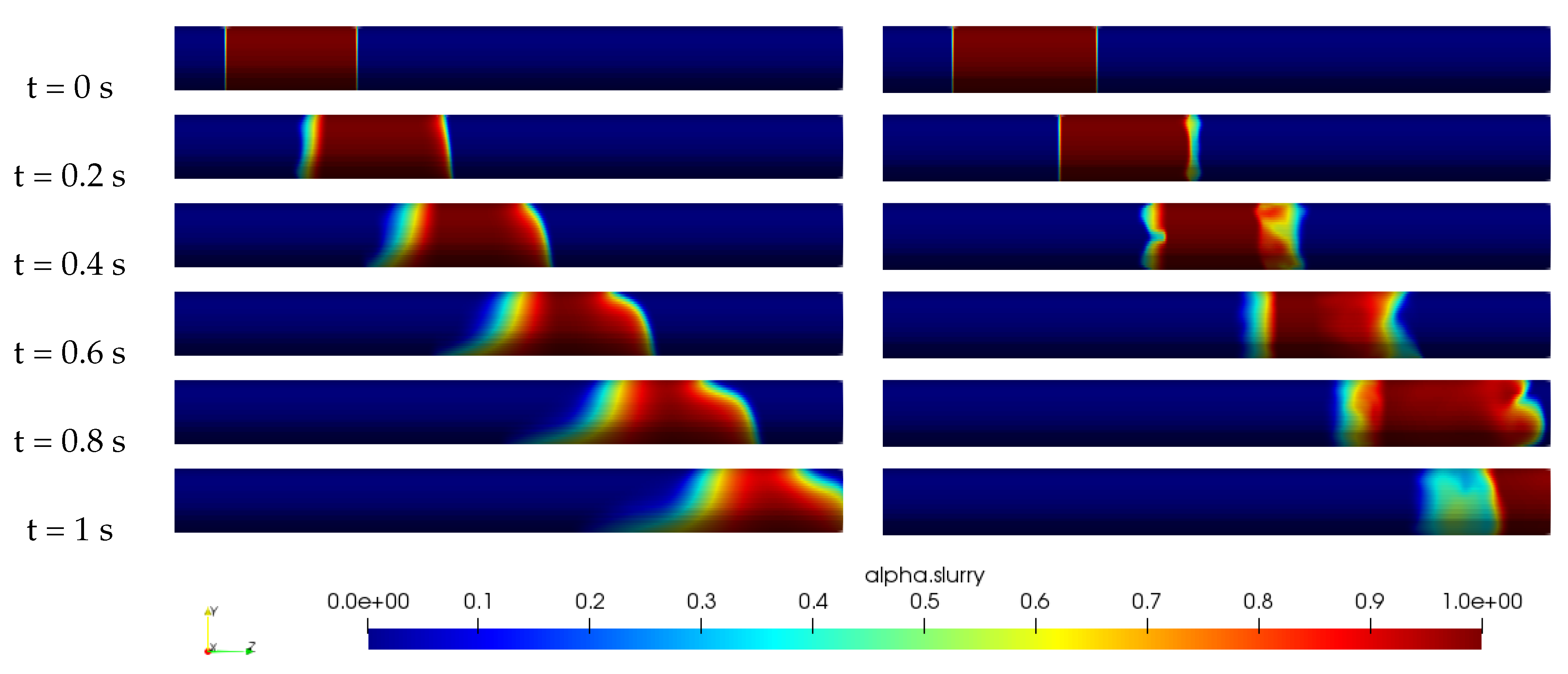
3.2.2. Two-Phase Pipe Flow

We recall that the configuration of interest in our work consists of a water-slurry batch flow, represented by Figure 6. A three-dimensional (3D) horizontal pipes are established to investigate the New rheological model of the particulate slurry flow using OpenFOAM simulations. Internal diameters D = 5.49 cm and D = 90 cm are used with corresponding pipe lengths L = 3.3 m and L = 50 m > 60 D respectively. The lengths of the slurry batch are respectively l = 0.54 m and l = 8.9 m. Table 4 represents physical characteristics of the two-phase system water-slurry. According to results in [29], the Herschel–Bulkley model is suitable for concentrations lower than 38.45 wt%, where the phosphate suspension rheological behavior is dilatant. The Casson model is used to model the rheological behavior of the suspension and to calculate the viscosity and yield strength for the concentration range ( 46.03 to 57.27 wt%). Therefore, the new model is compared to the Herschel–Bulkley model for the concentration C = 38.45 wt% by mass, and to the Casson model in the range of concentrations C = 46.03–57.27 wt%.
In order to validate our new model for phosphate slurry flow visualization, we compared it to the well-established Newtonian model using high mesh resolution (2 million cells), due to the limited experimental data available on this subject. The simulations were performed in a pipe with a diameter of D = 0.9 m and a length of L = 50 m, with a mean flow velocity of U = 5 m/s to achieve high turbulent flow. This was carried out in order to replicate the conditions often found in industrial settings where phosphate slurry is transported. Using the least squares method, we obtained consistency index of 1.56 and flow index of 0.01 , which correspond to a concentration of 56 wt%. These results demonstrate that our new model is a reliable and accurate representation of the rheology of phosphate slurry flow and can be used in industrial settings to better predict and control the flow of this fluid.
Figure 7 illustrates a detailed comparison of the distribution of slurry concentration between the Newtonian and new models, along a horizontal pipe. The Newtonian model is used as a reference solution for validation, as it is a well-established model and there is currently no other reference solution available in literature to validate the new model.
Upon examination of the figure, it is clear that the new model provides significantly improved results in comparison to the Newtonian model. One of the most notable differences is the absence of mixing at the interface between water and slurry in the case of the new model. This indicates that the new model is able to capture the behavior of the slurry more accurately and can be used to make more accurate predictions about the behavior of the slurry in industrial settings.
Additionally, the new model has the ability to predict the slurry concentration distribution at different sections of the pipe, which can be used to optimize the design and operation of industrial systems that transport phosphate slurry. The new model can also be used to improve the control of the flow of the slurry in real-world applications.
In conclusion, the new model for phosphate slurry flow visualization has been validated and compared to the Newtonian model with high accuracy. The results of the simulation demonstrate that this new model can be used to better predict and control the flow of phosphate slurry in industrial settings.
The Figure 8 and Figure 9 provide a comprehensive comparison of the distribution of slurry concentration along a horizontal pipe between the Herschel–Bulkley model, the Casson model, and the new model. The new model uses parameters a and b that are specific to the concentration of the slurry. For a concentration of 38.45 wt%, the values of a and b are respectively 0.4 Pa·s and 0.2 , and for C = 56 wt%, the values are a = 1.56 Pa·s and b = 0.6 . Upon examination of the figures, it can be seen that the new model is able to maintain the slurry batch compact until it exits the pipe, regardless of the concentration of the slurry. In contrast, the Herschel–Bulkley and Casson models exhibit mixing at the water-slurry interface and sedimentation of the slurry batch towards the bottom of the pipe. This suggests that the new model captures the rheological behavior of the phosphate suspension more accurately than the other models, especially for both low and high concentrations. In summary, the new model for phosphate slurry flow visualization has been compared to the Herschel–Bulkley model and Casson model and it has been found that it is able to reproduce well the rheological behavior of phosphate suspensions for both low and high concentrations. The new model can be used to improve predictions and control of the flow of phosphate slurry in industrial settings.

4. Conclusions

A new rheological constitutive relation for modeling the phosphate slurry flows was presented in this study. This model is based on five constant parameters, which were determined through rheological measurements. The validity of the model was assessed by comparing its outputs with data derived from stress test measurements. It was found that there was a good fit between the model and the measurements in the stress versus strain rate curves.
Furthermore, it was shown that the new model gives good numerical results when implemented in the OpenFoam software, version 9.0, and tested with an existing tutorial case model. The model was also validated numerically by comparing its concentration distribution results with those of the Newtonian model for high mesh resolution. It was found that the new model provides improved results compared to the Newtonian model. Additionally, the new model was compared to the Herschel–Bulkley model for a low concentration of C = 38.45 wt% and to the Casson model for C = 56 wt%. It was found that the new model was able to simulate the rheological behavior of phosphate slurry flows accurately for both low and high concentrations.
The main advantages of this new model are that it can produce improved fits of the rheological data compared to other existing models, and that it provides a description of the rheological behavior of the phosphate suspension for a wide range of concentrations. This makes it a valuable tool for understanding and predicting the behavior of phosphate slurry flows in industrial settings and for optimizing the design and operation of systems that transport phosphate slurry.

Author Contributions

Conceptualization, Z.G., S.M., F.B. and N.H.; methodology, Z.G., S.M., F.B. and N.H.; software, Z.G.; validation, Z.G., S.M.; formal analysis, Z.G.; investigation, Z.G., S.M., F.B. and N.H.; resources, Z.G., S.M., F.B. and N.H.; data curation, Z.G. and S.M.; writing—original draft preparation, Z.G. and S.M.; writing—review and editing, Z.G., S.M., F.B. and N.H.; visualization, F.B.; supervision, F.B. and N.H.; project administration, F.B. All authors have read and agreed to the published version of the manuscript.

Funding

This research received no external funding.

Institutional Review Board Statement

Not applicable.

Informed Consent Statement

Not applicable.

Data Availability Statement

The data presented in this study are available on request from the corresponding author.

Acknowledgments

The authors gratefully acknowledge the support and computing resources from The computing cluster MAGI at University of Paris 13.

Conflicts of Interest

The authors declare no conflict of interest.

References

  1. Bureš, L.; Sato, Y. Direct numerical simulation of evaporation and condensation with the geometric VOF method and a sharp-interface phase-change model. Int. J. Heat Mass Transf. 2021, 173, 121233. [Google Scholar] [CrossRef]
  2. Zhang, C.; Tan, J.; Ning, D. Machine learning strategy for viscous calibration of fully-nonlinear liquid sloshing simulation in FLNG tanks. Appl. Ocean. Res. 2021, 114, 102737. [Google Scholar] [CrossRef]
  3. Saghi, R.; Hirdaris, S.; Saghi, H. The influence of flexible fluid structure interactions on sway induced tank sloshing dynamics. Eng. Anal. Bound. Elem. 2021, 131, 206217. [Google Scholar] [CrossRef]
  4. Silvi, L.D.; Chandraker, D.K.; Ghosh, S.; Das, A.K. Understanding dry-out mechanism in rod bundles of boiling water reactor. Int. J. Heat Mass Transf. 2021, 177, 121534. [Google Scholar] [CrossRef]
  5. Vångö, M.; Pirker, S.; Lichtenegger, T. Unresolved CFD–DEM modeling of multiphase flow in densely packed particle beds. Appl. Math. Model. 2018, 56, 501–516. [Google Scholar] [CrossRef]
  6. Giussani, F.; Piscaglia, F.; Saez-Mischlich, G.; Helie, J. A three-phase VOF solver for the simulation of in-nozzle cavitation effects on liquid atomization. J. Comput. Phys. 2020, 406, 109068. [Google Scholar] [CrossRef]
  7. Di Iorio, S.; Catapano, F.; Magno, A.; Sementa, P.; Vaglieco, B.M. Investigation on sub-23 nm particles and their volatile organic fraction (VOF) in PFI/DI spark ignition engine fueled with gasoline, ethanol and a 30% v/v ethanol blend. J. Aerosol Sci. 2021, 153, 105723. [Google Scholar] [CrossRef]
  8. Sussman, M.; Smereka, P.; Osher, S. A level set approach for computing solutions to incompressible two-phase flow. J. Comput. Phys. 1994, 114, 146–159. [Google Scholar] [CrossRef]
  9. Hirt, C.W.; Nichols, B.D. Volume of fluid (VOF) method for the dynamics of free boundaries. J. Comput. Phys. 1981, 39, 201–225. [Google Scholar] [CrossRef]
  10. Kraposhin, M.V.; Banholzer, M.; Pfitzner, M.; Marchevsky, I. A hybrid pressure-based solver for nonideal single-phase fluid flows at all speeds. Int. J. Numer. Methods Fluids 2018, 88, 79–99. [Google Scholar] [CrossRef]
  11. Yu, C.-H.; Wen, H.L.; Gu, Z.H.; An, R.D. Numerical simulation of dam-break flow impacting a stationary obstacle by a CLSVOF/IB method. Commun. Nonlinear Sci. Numer. Simul. 2019, 79, 104934. [Google Scholar] [CrossRef]
  12. Jafari, E.; Namin, M.M.; Badiei, P. Numerical simulation of wave interaction with porous structures. Appl. Ocean. Res. 2021, 108, 102522. [Google Scholar] [CrossRef]
  13. Garoosi, F.; Mellado-Cusicahua, A.N.; Shademani, M.; Shakibaeinia, A. Experimental and numerical investigations of dam break flow over dry and wet beds. Int. J. Mech. Sci. 2022, 215, 106946. [Google Scholar] [CrossRef]
  14. Zhang, W.; Wang, J.; Yang, S.; Li, B.; Yu, K.; Wang, D.; Yongphet, P.; Xu, H. Dynamics of bubble formation on submerged capillaries in a non-uniform direct current electric field. Colloids Surfaces A Physicochem. Eng. Asp. 2020, 606, 125512. [Google Scholar] [CrossRef]
  15. Li, T.; Wang, S.; Li, S.; Zhang, A.-M. Numerical investigation of an underwater explosion bubble based on FVM and VOF. Appl. Ocean. Res. 2018, 74, 49–58. [Google Scholar] [CrossRef]
  16. Das, S.; Weerasiri, L.D.; Yang, W. Influence of surface tension on bubble nucleation, formation and onset of sliding. Colloids Surfaces A Physicochem. Eng. Asp. 2017, 516, 23–31. [Google Scholar] [CrossRef]
  17. Yang, C.; Cao, W.; Yang, Z. Study on dynamic behavior of water droplet impacting on super-hydrophobic surface with micro-pillar structures by VOF method. Colloids Surfaces A Physicochem. Eng. Asp. 2021, 603, 127634. [Google Scholar] [CrossRef]
  18. Hanene, Z.; Alla, H.; Abdelouahab, M.; Roques-Carmes, T. A numerical model of an immiscible surfactant drop spreading over thin liquid layers using CFD/VOF approach. Colloids Surfaces A Physicochem. Eng. Asp. 2020, 600, 124953. [Google Scholar] [CrossRef]
  19. de Lima, B.S.; Meira, L.d.; Souza, F.J.d. Numerical simulation of a water droplet splash: Comparison between PLIC and HRIC schemes for the VoF transport equation. Eur. J. -Mech.-B/Fluids 2020, 84, 63–70. [Google Scholar] [CrossRef]
  20. Yun, S. Ellipsoidal drop impact on a single-ridge superhydrophobic surface. Int. J. Mech. Sci. 2021, 208, 106677. [Google Scholar] [CrossRef]
  21. Kalifa, R.B.; Hamza, S.B.; Said, N.M.; Bournot, H. Fluid flow phenomena in metals processing operations: Numerical description of the fluid flow field by an impinging gas jet on a liquid surface. Int. J. Mech. Sci. 2020, 165, 105220. [Google Scholar] [CrossRef]
  22. Frigaard, I. Simple yield stress fluids. Curr. Opin. Colloid Interface Sci. 2019, 43, 80–93. [Google Scholar] [CrossRef]
  23. Bingham, E.C. Fluidity and Plasticity; McGraw-Hill: New York, NY, USA, 1922. [Google Scholar]
  24. Herschel, W.H.; Bulkley, R. Konsistenzmessungen von gummi-benzollösungen. Kolloid-Zeitschrift 1926, 39, 291–300. [Google Scholar] [CrossRef]
  25. Casson, N. A flow equation for pigment-oil suspensions of the printing ink type. Rheol. Disperse Syst. 1959, 84–104. [Google Scholar]
  26. Tanner, R.I. Rheology of noncolloidal suspensions with non-Newtonian matrices. J. Rheol. 2019, 63, 705–717. [Google Scholar] [CrossRef]
  27. Zhang, Z.; Ye, S.; Yin, B.; Song, X.; Wang, Y.; Huang, C.; Chen, Y. A semi-implicit discrepancy model of Reynolds stress in a higher-order tensor basis framework for Reynolds-averaged Navier–Stokes simulations. AIP Adv. 2021, 11, 045025. [Google Scholar] [CrossRef]
  28. Dai, S.-C.; Bertevas, E.; Qi, F.; Tanner, R.I. Viscometric functions for noncolloidal sphere suspensions with Newtonian matrices. J. Rheol. 2013, 57, 493–510. [Google Scholar] [CrossRef]
  29. Belbsir, H.; El-Hami, K.; Soufi, A. Study of the rheological behavior of the phosphate-water slurry and search for a suitable model to describe its rheological behavior. Int. J. Mech. Mechatron. Eng. IJMME-IJENS 2018, 18, 73–81. [Google Scholar]
  30. Zhang, S.; Jiang, B.; Law, A.W.; Zhao, B. Large eddy simulations of 45 inclined dense jets. Environ. Fluid Mech. 2016, 16, 101–121. [Google Scholar] [CrossRef]
  31. Krpan, R.; Končar, B. Simulation of turbulent wake at mixing of two confined horizontal flows. Sci. Technol. Nucl. Install. 2018, 2018, 5240361. [Google Scholar] [CrossRef]
  32. Jasak, H.; Jemcov, A.; Tukovic, Z. OpenFOAM: A C++ library for complex physics simulations. In Proceedings of the International Workshop on Coupled Methods in Numerical Dynamics, IUC, Dubrovnik, Croatia, 19–21 September 2007. [Google Scholar]
  33. Palmore, J., Jr.; Desjardins, O. A volume of fluid framework for interface-resolved simulations of vaporizing liquid-gas flows. J. Comput. Phys. 2019, 399, 108954. [Google Scholar] [CrossRef]
  34. Brackbill, J.U.; Kothe, D.B.; Zemach, C. A continuum method for modeling surface tension. J. Comput. Phys. 1992, 100, 335–354. [Google Scholar] [CrossRef]
  35. Menter, F.R. Two-equation eddy-viscosity turbulence models for engineering applications. AIAA J. 1994, 32, 1598–1605. [Google Scholar] [CrossRef]
  36. Launder, B.E.; Spalding, D.B. The numerical computation of turbulent flows. In Numerical Prediction of Flow, Heat Transfer, Turbulence and Combustion; Elsevier: Amsterdam, The Netherlands, 1983; pp. 96–116. [Google Scholar]
  37. Henkes, R.A.W.M.; Van Der Vlugt, F.F.; Hoogendoorn, C.J. Natural-convection flow in a square cavity calculated with low-Reynolds-number turbulence models. Int. J. Heat Mass Transf. 1991, 34, 377–388. [Google Scholar] [CrossRef]
  38. Yakhot, V.; Smith, L.M. The renormalization group, the ϵ-expansion and derivation of turbulence models. J. Sci. Comput. 1992, 7, 35–61. [Google Scholar] [CrossRef]
  39. Menter, F.R. Turbulence Modeling for Engineering Flows; Ansys, Inc.: Canonsburg, PA, USA, 2011. [Google Scholar]
  40. Maazioui, S.; Maazouz, A.; Benkhaldoun, F.; Ouazar, D.; Lamnawar, K. Rheological Characterization of a Concentrated Phosphate Slurry. Fluids 2021, 6, 178. [Google Scholar] [CrossRef]
  41. Maazioui, S.; Kissami, I.; Benkhaldoun, F.; Ouazar, D. Numerical Study of Viscoplastic Flows Using a Multigrid Initialization Algorithm. Algorithms 2023, 16, 50. [Google Scholar] [CrossRef]
  42. Guadagni, S.; Palade, L.I.; Fusi, L.; Farina, A. On a Casson fluid motion: Nonuniform width symmetric channel and peristaltic flows. Fluids 2021, 6, 356. [Google Scholar] [CrossRef]
Figure 1. Comparison of experimental (red circles) and predicted (blue cross) values of shear stress as a function of shear rate for six phosphate slurry test samples.
Fluids 08 00057 g001
Figure 2. Slurry concentration distribution inside an inviscid walls column, Newtonian Model.
Fluids 08 00057 g002
Figure 3. Slurry concentration distribution inside an inviscid walls column, Herschel-Bulkley Model.
Fluids 08 00057 g003
Figure 4. Slurry concentration distribution inside an inviscid walls column, Casson Model.
Fluids 08 00057 g004
Figure 5. Slurry concentration distribution inside an inviscid walls column, New Model, a = 0.93 Pa·s, b = 0.49 .
Fluids 08 00057 g005
Figure 6. Flow configuration in the horizontal pipeline.
Fluids 08 00057 g006
Figure 7. Slurry concentration distribution along the pipe for D = 0.9 m, U = 5 m/s, C = 56 wt%, a = 1.56 Pa·s, b = 0.01 , Newtonian model (left) and the New model (right).
Fluids 08 00057 g007
Figure 8. Slurry concentration distribution across the pipe for D = 54.9 mm, U = 2 m/s, C = 38.45 wt%, a = 0.4 Pa·s, b = 0.2 , Herschel–Bulkley model (left) and the New model (right).
Fluids 08 00057 g008
Figure 9. Slurry concentration distribution across the pipe for D = 54.9 mm, U = 2 m/s, C = 56 wt%, a = 1.56 Pa·s, b = 0.01 , Casson model (left) and the New model (right).
Fluids 08 00057 g009
Table 1. The two-phase system used.
MaterialDensityKinematic ViscosityRheological Model
(kg/m 3 )(m 2 /s)
Water990 1.00 × 10 6 Newtonian
Sludge1000 6.00 × 10 6 Newtonian
non-constantHerschel–Bulkley, Casson and New Model
Table 2. Specification of the multiphase solver used.
TermDetails
Name of solvertwoLiquidMixingFoam
Type of solverDensity-based, segregated solver
Time dependencyTransient
Pressure-velocity couplingPimple
nCorrectors3
nNonOrthogonalCorrector0
Table 3. Constant parameters of the new model.
ModelPhosphate Slurry Samples
ParametersS1S2S3S4S5S6
a [Pa·s b ]0.930.440.720.571.601.56
η [mPa·s]16.7718.3323.2623.627.4530.8
b [-]0.490.590.600.570.560.59
τ c [Pa]10.207.5115.3811.0331.1637.39
γ ˙ 0 [1/s]12.546.222.4222.7818.4615.26
Table 4. Ranges of parametric values.
ParametersRangesUnit
Pipe diameter0.054–0.9m
Pipe Length3.3–50m
Solid concentration by mass38–56wt%
Water density1000kg/m 3
Water viscosity 10 3 Pa·s
Velocity2–5m/s
Water Reynolds Number> 10 6 -
Disclaimer/Publisher’s Note: The statements, opinions and data contained in all publications are solely those of the individual author(s) and contributor(s) and not of MDPI and/or the editor(s). MDPI and/or the editor(s) disclaim responsibility for any injury to people or property resulting from any ideas, methods, instructions or products referred to in the content.

