Article

Interfacial Dynamics of Miscible Displacement of Shear-Thinning Fluid in a Vertical Channel

by
Yao Zhang
,
Andrianifaliana H. Rabenjafimanantsoa
and
Hans Joakim Skadsem
*
Department Energy and Petroleum Engineering, University of Stavanger, NO-4068 Stavanger, Norway
*
Author to whom correspondence should be addressed.
Fluids 2023, 8(2), 35; https://doi.org/10.3390/fluids8020035
Submission received: 12 December 2022 / Revised: 9 January 2023 / Accepted: 16 January 2023 / Published: 18 January 2023
(This article belongs to the Collection Non-Newtonian Fluid Mechanics)

Abstract

:
The displacement of a shear-thinning fluid by a denser and less viscous Newtonian fluid in a vertical duct is investigated using experiments and numerical simulations. We study how shear-thinning and increased viscosity contrast between the fluids affect the displacement. Our results show that the degree of shear-thinning significantly influences the development of interfacial patterns and the growth of perturbations. In the weakly shear-thinning regime, the displacement progresses as a stable displacement with no visible instabilities. Increasing the viscosity of the displaced fluids result in a Saffman–Taylor type instability with several finger-shaped channels carved across the width of the duct. In the strongly shear-thinning regime, a unique viscous finger with an uneven interface is formed in the middle of the displaced fluid. This finger eventually breaks through at the outlet, leaving behind considerably stagnant wall layers at the duct side walls. We link the onset of viscous fingering instability to the viscosity contrast between the fluids, and the stabilizing density difference, as expressed through a modified, unperturbed pressure gradient for the two fluids. Numerical simulations are performed with both an initial flat interface, and with a perturbed interface, and we find good qualitative agreement between experimental observations and computations.

1. Introduction

The displacement of one fluid by another is a flow process with implications to engineering, industrial and medical applications. Many of these displacement flows involves non-Newtonian fluids and fluid pairs with large viscosity contrasts [1,2,3,4,5]. While non-Newtonian fluid properties, such as shear-thinning or yield stress behavior, can be deliberately introduced into fluids to improve the displacement process, the resulting non-linearity complicates the analysis of the displacement. Of particular importance for several industrial applications is the ability to predict the stability of the interfacial dynamics of a certain displacement process [6,7], i.e., to predict the dissipation of interfacial waves [8]; whether the amplitude of perturbations to the flow will grow or dissipate over time [9]; and to analyze the velocity field and energy transformation around a Taylor bubble [10]. Example instabilities include the classical Rayleigh–Taylor and Saffman–Taylor instabilities, which are associated with density- and viscosity-unstable conditions. The topic of the current study is the upward displacement of a viscous, non-Newtonian fluid by a less viscous Newtonian fluid, and is therefore connected to the Saffman–Taylor instability where fingers of the displacing fluid may penetrate into the more viscous, displaced fluid [11,12].
Viscous fingering and related instabilities have frequently been studied in Hele-Shaw cells that consist of wide parallel plates separated by a narrow gap, h. It follows from momentum conservation that the mean velocity, U , of a Newtonian fluid in a Hele-Shaw cell is U = h 2 p / 12 μ , with μ the fluid viscosity and p is the pressure. This equation is identical to the so-called Darcy equation that is often used when studying non-inertial flow in permeable porous media, with h 2 / 12 corresponding to the media permeability [12,13]. The Hele-Shaw geometry therefore represents an attractive and relevant measurement geometry for studying porous media displacements, which are important for optimizing increased oil recovery processes or the geological sequestriation of carbon dioxide.
The stability of the interface between two superposed fluids that are subject to a pressure gradient was studied in the classical paper of Taylor and Saffman [11]. For Newtonian fluids and in the absence of gravity and interfacial tension, the flow becomes unstable to linear perturbations when the displacing fluid is less viscous than the displaced fluid [14], resulting in the penetration and growth of viscous fingers into the displaced fluid. In upward, vertical flow in the presence of gravity, a density difference between the fluids will also affect the stability of the flow by suppressing viscous fingering when the lower, displacing fluid is denser than the displaced fluid. Denoting the displaced, upper fluid by 2 and the displacing, lower fluid by 1, the displacement becomes unstable to perturbations when ρ 1 g + μ 1 U 0 / k 1 > ρ 2 g + μ 2 U 0 / k 2 , as shown by, e.g., Leal [14]. Here, ρ i and k i correspond to the density and permeability of fluid i, respectively, g is the gravitational acceleration and U 0 is the magnitude of the imposed flow velocity. As pointed out above, for a Hele-Shaw cell of uniform gap width, k i h 2 / 12 , and μ i U 0 / k i corresponds to the (unperturbed) friction pressure gradient of fluid i. As such, the displacement becomes unstable when the “modified” pressure gradient of the displaced fluid exceeds that of the displacing fluid. According to this criterion, a density-unstable configuration ( ρ 2 > ρ 1 ) can be stabilized by viscosifying the displacing fluid: μ 1 μ 2 > ( ρ 2 ρ 1 ) g k / U 0 . Similarly, a viscosity-unstable configuration ( μ 2 > μ 1 ) can be stabilized by increasing the density of the displacing fluid: ρ 1 ρ 2 > ( μ 2 μ 1 ) U 0 / ( g k ) [15]. In this study, we will connect this stability criterion to the density-stable and viscosity-unstable displacement of a shear thinning fluid.
The Hele-Shaw geometry and the Saffman–Taylor instability is relevant also for fluid displacements in narrow annulus geometries. Indeed, to leading order in the gap width, displacements in a narrow, eccentric annulus can be approximated by displacements in an equivalent Hele-Shaw cell of varying gap-width [5,9,14]. The cementing of casing strings during well construction is an example of annular fluid displacement with significant industrial and environmental importance. The cementing operation involves displacement of a drilling fluid from the annulus, and the placement of a cement slurry that should form a barrier for zonal isolation behind the cemented casing string. To prevent instabilities and optimize the displacement efficiency, industry guidelines for displacements in vertical or inclined annuli generally recommend that the displacing fluids should be denser and exert a greater friction pressure than the fluids they displace [16]. While gravity will act to stabilize displacements in vertical and inclined geometries (the displacing cement slurry being denser and displacing lighter fluids upward), the viscosity hierarchy between fluids is considered particularly important for the cementing of horizontal and near-horizontal annuli. Indeed, within a lubrication scaling, Carrasco-Teja et al. showed that conditions for the existence of steady displacements in horizontal annuli is given entirely by the viscosity of the two fluids [17].
Since the classical work by Taylor and Saffman [11], many experimental studies have explored the growth of viscous fingering instabilities and displacement mechanics in the Hele-Shaw cell geometry. In a comprehensive review, Homsy illustrated the morphology of viscous fingering at the liquid interface for both miscible and immiscible displacement in Hele-Shaw cells [12]. The dynamics of viscous fingering, i.e., splitting, shielding, spreading and its relevant dimensionless numbers were discussed in detail. McCloud and Maher made an in-depth experimental study on the perturbations to viscous fingering with a Hele-Shaw cell [18]. Density-stable downward displacements of Newtonian liquids in a vertical Hele-Shaw cell was studied experimentally and theoretically by Lajeunesse et al., who focused on sufficiently high flow rates for capillary effects to be small [19]. In this limit, the interface that separates the fluids does not necessarily span across the gap of the Hele-Shaw cell, and the profile of the interface may develop inside the gap. Using a lubrication scaling [19], derived a hyperbolic conservation equation for the gap-wise shape of the interface, and predicted three qualitatively different interface shapes depending on the viscosity ratio between the fluids, and the ratio of viscous to buoyant forces. Subsequently, Fernandez et al. explored density-driven flow and instability in a similar vertical Hele-Shaw cell [20]. Haudin et al. further studied buoyancy-driven instabilities in viscously stable miscible displacements within a horizontal Hele-Shaw cell [21]. An et al. in their recent work studied miscible viscous fingering in a sealed Hele-Shaw cell, where they explored how different parameters can effect the viscous finger dynamics, and identified different flow regimes and their fingering characteristics [22].
As the Saffman–Taylor instability is strongly linked to the viscosity of the two fluids, one can expect non-Newtonian properties in either of the two fluids to impact the displacement stability and the criterion for onset of viscous fingering instability. A linear stability analysis for the displacement by air of an Oldroyd ’Fluid B’ model or a power law fluid was performed by Wilson [13]. shear-thinning was found to modify the growth rate of perturbations to the fluid-fluid interface by a factor of n 1 / 2 , with n being the flow behavior index of the displaced, power law fluid [13]. Subsequently, Mora and Manna performed a linear stability analysis involving two non-Newtonian fluids in a horizontal Hele-Shaw cell [23], and for air displacing a viscoelastic Maxwell fluid [24]. From a Darcy relation for generalized Newtonian fluids, their linear stability analysis showed that interfacial perturbations grow when the unperturbed pressure gradient of the displaced fluid exceeds that of the displacing fluid and the stabilizing effect of interfacial tension [23]. Thus, this stability criterion for generalized Newtonian fluids is analogous to that of Newtonian fluids, as discussed above.
An experimental investigation of the impact of non-Newtonian viscosity on viscous fingering instability was reported by Lindner et al., who performed experiments with solutions containing rigid (shear-thinning) or flexible (elastic) polymer solutions [25]. Their results showed that a modified Darcy equation could explain the relative finger width observed in solutions with low polymer concentration [25]. A recent experimental study considered displacements involving a Newtonian mineral oil and aqueous shear-thinning liquids in a horizontal Hele-Shaw cell [26]. The experiments showed that a transition from viscous fingering to stable plug displacement occurred for viscosity ratios between displacing and displaced fluid of approximately 2.25–2.5. That is, fingering instabilities could still occur even if the viscosity of the displacing fluid is more than twice that of the wall viscosity of the displaced fluid. Varges et al. attributed these observations to the shear-thinning property of the aqueous solution, i.e., the existence of viscosity gradients across the gap in the Hele-Shaw cell, with the shear-thinning fluid having a significantly larger effective viscosity close to the center of the gap compared to at the walls [26]. We remark that these observations appear to be (at least qualitatively) in agreement with the stability criterion developed by Mora and Manna [23], which relates the stability of the to unperturbed friction pressure gradients and not the fluid viscosity function directly. Even more recently, Jiang et al. performed an experimental study that investigated the effect of polymeric liquid additives on the onset of viscous fingering as well as finger shapes [27]. Their results confirmed the observations of the previous study, i.e., that viscous fingering may occur even when the displaced, shear-thinning fluid has an effective viscosity less than the viscosity of the displacing, Newtonian fluid, and that this is linked to the viscosity gradient in the gap [27]. Further, and as discussed by, e.g., Lindner et al. [28], it has been observed that rigid polymers and flexible polymers affect finger width differently: Rigid polymer solutions that exhibit viscous fingering, tend to develop narrower fingers at higher imposed velocity due to shear thinning at the finger tip. This results in lower local viscosity at the tip and easier growth of a narrow finger. Flexible polymer solutions, on the other hand, show larger resistance to elongation and a tendency for developing wider fingers [28].
Finally, we comment that recent work has also investigated impacts of surfactants on viscous finger formation at the interface between immiscible fluids. Bonn et al. showed that addition of surfactants increased the width of the viscous finger formed as heptane displaced water [29]. This observation can be explained by surface tension anisotropy along the interface caused by a competition of advection and adsorption of surfactant molecules, resulting in maximum surface tension at the tip and minimum at the sides, [29]. Ahmadikhamsi et al. recently studied the combination of surfactants and non-Newtonian viscosity on viscous fingering in a radial Hele-Shaw cell where an aqueous polymer solution displaced a viscous oil [30]. Similar to the case with Newtonian fluids, this study also found a tendency for wider-finger formation caused by surface tension anisotropy. In contrast to Newtonian displacements, shear thinning was found to increase the finger width for increasing flow rate [30]. Research efforts on theoretical and physical principles regarding the effects of the addition of surfactants on viscosity and forces at the interface, as well as the interfacial rheology are addressed in, e.g., Refs. [31,32,33,34], and a comprehensive review of surfactant dynamics was provided by Manikantan and Squires [7].
As addressed in recent literature, additional experimental and theoretical studies on the subject are required to evaluate criteria for onset of viscous fingering instabilities, and the resulting finger morphology [12,18,25], especially for displacements that involve one or more non-Newtonian fluids. In this work, we report a combined experimental and numerical investigation of the interface dynamics for the viscosity-unstable displacement of a shear-thinning fluid by a denser Newtonian fluid. The goals of this work are to connect the fingering instability to viscosity- and density-differences between the two fluids, and to qualitatively validate numerical simulations of these displacements.

2. Methodology

2.1. Experimental Geometry

Our experimental test setup consists of a rectangular duct with a cross section of 0.17 m width and 0.017 m narrow gap. The height of the duct is 1 m. A schematic of the experimental setup is shown in Figure 1.
The interface between two fluids was set initially at 60 cm above the inlet (bottom) of the duct. A specially designed mechanical separation device was used to ensure minimial initial mixing between the two fluids, and to achieve a well-defined and repeatable horizontal fluid interface at the start of the experiment. The displacing fluid was colored with black ink for visualization purposes. Flow visualization set on the front side of the duct, and is the achieved by high-speed video imaging with a high intensity lighting source. We used an LED lighting panel as the lighting source. It was placed behind the duct during the experiments to light the displaced fluid section as shown in Figure 1. The high-speed camera is set front of the duct, directly opposite to the lighting source. The lighting panel allows uniform light distribution, at the same time prevent the creation of concentrated lighting spot and overexposure.
This laboratory setup was designed and constructed to ensure precise control of inlet flow velocity and to provide optical access for flow visualization. A goal of the design was to enable direct comparison between measurements and corresponding numerical simulations for validation purposes. We note that the aspect ratio of the confined channel, i.e., the ratio of width to gap length, λ = W / h , is 10. The resulting channel is therefore not a classical Hele-Shaw cell, but instead a rectangular channel where we expect fully three-dimensional effects to be present. The choice of the geometric dimensions was motivated in part by having a gap width comparable to the annular clearance between casings for primary cementing, but also for potential future study of gap-wise displacement mechanics. We comment that the short side walls of the channel will affect the flow in their proximity and away from the center part of the channel, and that the relatively wide gap (0.017 m) suggests that inertial effects may not be neglected, at least not in the least viscous fluid used in this study.

2.2. Fluid and Flow Properties

The displacing fluid in the experiment was plain tap water densified with a small addition of NaCl to reach a mass density of 1000 kg/m 3 . The corresponding viscosity for the displacing fluid at room temperature was 0.001 Pa·s. Different concentration aqueous xanthan gum solutions were prepared as the displaced fluid. We have considered displaced fluid with xanthan gum concentrations of 0.02%, 0.075% and 0.225% by weight. The increasing concentration of xanthan gum results in a higher degree of shear-thinning, and we refer to these displaced fluids as weakly, moderate and highly shear-thinning, respectively. Xanthan gum was chosen as viscosifier, as it is a commonly used additive in petroleum, pharmaceutical, and food industries. Xanthan gum is a high molecular weight polysaccharide which, when added to a liquid, quickly disperses and creates a viscous and stable solution [35].
Xanthan gum solutions are shear-thinning fluids, and its steady state flow curve is well described by a power law, or Ostwald–de Waele equation [36], i.e., τ = κ γ ˙ n , where τ and γ ˙ denote the shear stress and shear rate, respectively, and κ and n are the consistency index and the flow behavior index of the power law model, respectively. The flow curves of the three different concentrations of xanthan gum solution were measured using an Anton Paar MCR302 scientific rheometer fitted with a concentric cylinder measurement geometry, and the measurements were fitted to the power law model described above. The resulting least squares model parameters are listed in Table 1. We note that when fitting the measurements to the alternative Herschel–Bulkley model, τ = τ 0 + κ γ ˙ n , with τ 0 denoting yield stress, we found τ 0 0 Pa, suggesting purely viscous, shear-thinning behavior. The mass density of the xanthan gum solutions was measured to be 998 kg/m 3 for all concentrations considered in this study. Fluid densities were measured with an Anton Paar DMA1001.

2.3. Experimental Procedure

Displacement experiments were performed at a fixed volumetric flow rate of 4.6 L/min for all cases. A centrifugal pump was used to pump the displacing fluid and an ultrasonic flowmeter from Sensata Technologies (model UF25) was used to measure the flow rate. This choice of flow rate ensured that the flow remained laminar in both phases. For each displacement experiment, the lower and upper parts of the duct were filled with displacing and displaced fluids, respectively, prior to the displacement process. The two fluids were separated using a specially designed gate to ensure that the interface was sharp at the start of the experiment. The gate was opened just before the displacing process starts.
A by-pass loop was created to ensure that the pump was already operating at a steady flow rate by the time the experiment began. Displacing fluid was directed through the by-pass loop at a constant flow rate that was known to deliver the desired flow rate after switching the valve and opening the gate. Right after opening the gate, the displacement process was started by simultaneously closing the by-pass valve and opening the main valve, thus allowing the pump to inject displacing fluid into the duct. The displacing fluid was thus injected from the bottom of the duct through a honeycomb flow straightener to reduce disturbance in the flow and homogenize the velocity profile. The displaced xanthan gum solution was pushed to the outlet on the top of the duct to enter waste fluid collector.

2.4. Dimensionless Parameters

Relevant dimensionless numbers that govern the displacement experiments can be found by nondimensionalizing the equations of mass and momentum conservation, and the usual convection-diffusion equation for fluid concentrations. The particular geometry of the rectangular duct is characterized by the duct aspect ratio, λ = W / h , which we define as the width relative to the gap size of the duct. In the current configuration, λ = 10 . To characterize the relevant inertial, buoyant and viscous stresses, we take the ratio of the imposed bulk velocity, U 0 , to the narrow gap width, h, as characteristic shear rate, γ ˙ * = U 0 / h , and associate an effective viscosity with the displaced fluid phase, i.e., μ 1 * = κ 1 γ ˙ * n 1 1 . The bulk velocity is defined as the imposed volumetric flow rate, Q, divided by the cross-sectional area of the duct, U 0 = Q / ( W h ) . The ratio of inertial and viscous stresses is given by the Reynolds number as R e = ρ ¯ U 0 2 / τ * , where ρ ¯ is the average mass density and where a characteristic shear stress is introduced as τ * = max { μ 1 * γ ˙ * , μ 2 γ ˙ * } . Similarly, the ratio of inertial and buoyant stresses is expressed by the densimetric Froude number, defined as F r 2 = U 0 2 / ( A t g h ) , with A t = ( ρ 1 ρ 2 ) / 2 ρ ¯ being the Atwood number. Table 2 provides a summary of the relevant dimensionless numbers for this study, along with typical range or value each. Finally, we point out that generalized Newtonian fluids tend to complicate the definition of, e.g., the Reynolds number for this fluid. Above, we have simply taken the ratio of the inertial and a fixed, characteristic viscous stress scale as our Reynolds number. We note that a different approach to defining this dimensionless number is that of Metzner and Reed, where a generalized Reynolds number, R e M R , is introduced that is defined so that the Darcy–Weisbach friction factor, f, is f = 64 / R e M R in the laminar regime [37]. We note that the latter definition of the Reynolds number suggest that the displacement experiments were within a laminar flow regime.

2.5. Computational Tools

2.5.1. Solver and Assumptions

We assume that the vertical fluid displacements considered in this study are governed by equations for mass and momentum conservation, and that the concentration of displacing fluid, c, evolves according to
c t + · ( c U ) = 0 ,
where U is the velocity vector. No diffusive term is included in Equation (1), as we will assume the time-scale for diffusive mixing to be significantly longer than the typical time-scale of our experiments. Further, assuming incompressible fluids, the equation for mass conservation requires the velocity field to be solenoidal:
· U = 0 .
Finally, the equation for momentum conservation reads:
ρ U t + · ( ρ U U ) = p + · ( 2 μ S ) + ρ g ,
where p, μ and g denote pressure, fluid viscosity and the gravitational acceleration, respectively, and where S = U + ( U ) T / 2 is the rate-of-strain tensor.
All numerical simulations for this study have been performed using OpenFOAM: an open-source CFD software with many useful modelling features. OpenFOAM provides several numerical solvers for multi-phase simulations, and the interIsoFoam has been used for the current study. This solver is an upgraded version of the volume-of-fluid (VOF) interFoam solver that features the isoAdvector method, which helps resolving sharp fluid interfaces [38]. The interIsoFoam solver was initially developed for modelling of incompressible, immiscible two-phase flows. In this study, this immiscible solver is picked so that interface dynamics between the fluids can be captured as clearly as possible in the numerical simulations. Treating the two fluids effectively as immiscible is considered reasonable as the time-scale for molecular diffusion should be considerably larger compared to the relevant advective time-scale of our experiments. Moreover, the flow around the interface is assumed for the most part laminar, which means that the clean interface that separates the fluids at t = 0 s is likely to be preserved throughout the experiments. Therefore, the fluid pair can be considered as “immiscible” so that the evolution of interface can be investigated. Note that the “immisible” interface hypothesis is evident from experimental observations shown in Section 3. When using interIsoFoam for miscible fluids, the setting for surface tension between two fluids should be lowered to a value near 0 N/m. the boundary conditions were chosen to take account of the
Finally, the boundary conditions were set to take account of the fact that the flow is internal. Consequently, the inlet features constant velocity reflecting the flow rate and cross-section area, and zero gradient for pressure. The boundary condition for the outlet uses zero gradient for velocity and a constant reference value for pressure. The non-slip boundary condition is applied at all walls.

2.5.2. Transport and Rheology Model

OpenFOAM offers many built-in options for non-Newtonian fluid models [39]. In accordance with the experimental measurements of displaced fluid viscosity, the power law model is chosen for the xanthan gum solutions. This feature is parametrized in the transport properties file of the OpenFOAM set up. The power law model assumes that the kinematic viscosity of the fluid is described by Equation (4), with κ being the flow consistency index and n being the flow behavior index of the power law fluid:
μ / ρ = ν = ( κ / ρ ) γ ˙ n 1 , ν m i n ν ν m a x .
Since ν as γ ˙ 0 for shear-thinning fluids, a maximum, numerical kinematic viscosity needs to be defined in the model, ν m a x . Similarly, since ν 0 as γ ˙ , a certain, minimum numerical viscosity, ν m i n is also defined. In our case, ν m i n and ν m a x are set to be small and large enough, respectively, to make sure the solver is robust and exhibits stable behavior, and that the effective viscosity of the displaced fluid is in accordance with the power law model over the active mesh.

2.5.3. Mesh Independence Study

Meshing was performed using the blockMesh tool that comes with OpenFOAM. A mesh independence study was conducted using seven different resolutions, and considering the displacement of the weakly shear-thinning fluid by the Newtonian fluid. The peak velocity magnitude at the end of the simulation was used as comparison parameter. The precision tolerance is set to be 10 6 .The results from mesh analysis is shown in Figure 2.
It is clear that there is a rapid decrease in the peak velocity magnitude when going from mesh M1 to mesh M4. Finer mesh refinements result in considerably smaller changes in the peak velocity (less than 5% reduction per mesh refinement). The final chosen mesh size is M6, which contains 20 cells across the gap, 160 cells along the width and 256 cells along the length of the channel. The mesh grid used for all CFD simulations is shown in Figure 3 which, as pointed out above, corresponds to the static mesh M6. A numerical convergence or precision criterion of 10 6 was satisfied at every iteration of every case presented in this work.

2.5.4. Parallel Computation

The results presented in this work were generated using 8 processors in parallel to cope with the intensity of computation. The models were run using a computer with 32 GB RAM and 8 cores (CPU: Intel i7-11700 @ 2.50 GHz). The mesh was divided across the height of the duct creating 8 evenly distributed blocks, each consisting of 102,400 cells. Parallelization reduced the computational times for all cases by 8 times for the defined precision tolerance 10 6 at each iteration of every case. The CPU times varied between 10,892 s to 22,183 s, depending on the level of shear-thinning of displaced fluid. The highest computational cost corresponded to the cases involving the strong shear-thinning fluid as shown in Figure 4. The lower computational cost corresponded to displacements with equivalent Newtonian viscosity as shown in Figure 5.

2.5.5. Perturbation of Initial Interface Shape

In the current study, simulations have been performed with an initial horizontal interface between the two fluids, as well as with an initially “perturbed” interface in the form of a sinusoidally varying interface shape. The module CodeStream is used to implement the induced perturbation at the interface. This module allows the generation of a custom, defined interface and boundary conditions. In this work, the “perturbed” initial interface is defined as z = z 0 + A sin ( 2 π x / λ ) , i.e., corresponding to a harmonic oscillation of amplitude A and wavelength λ about the mean height z 0 above the inlet to the duct. The details of sinusoidal wave function used to define the initial shape of the interface is addressed in Section 3.2.

3. Results and Analysis

3.1. Interface Shape during Displacement of Shear-Thinning Fluids

3.1.1. Weakly Shear-Thinning Regime

Shown in the top panel of Figure 5 is a visualization of the fluid-fluid interface at different times since start of the displacement experiment for the weakly shear-thinning displaced fluid. In the central panel, equivalent results are shown for the simulations of this case, while the bottom panel corresponds to numerical simulations involving the displacement of a Newtonian fluid of the same effective viscosity as the power law fluid. The effective Newtonian viscosity is estimated based on the characteristic shear rate γ ˙ * = 3 U 0 / h = 4.69 s 1 , with U 0 the bulk velocity, and h is the gap width of the duct. After obtaining the shear rate, the equivalent Newtonian viscosity is taken as μ * = κ γ ˙ n 1 . Simulations from two models show very similar results and appear to agrees well with what is observed from the experiment. Both the fluid interface dynamics and the displacement process behaved like the two-phase flow of Newtonian fluid.
The interface advanced steady and uniformly along the duct in experiment and numerical simulations, characteristic of a stable displacement. Comparison of the numerical simulations suggest minor effect of shear-thinning on the interface shape, as expected since the small concentration of xanthan gum only imparts a modest degree of shear-thinning in the displaced fluid. Interestingly, we note that no obvious viscous fingering instability occur, even if the displaced fluid is considerably more viscous than the displacing water phase. We will argue below that the density difference between the fluids is here sufficient to suppress the development of fingering instabilities.

3.1.2. Moderately Shear-Thinning Regime

Visualization of the interface shape for displacement of the moderately shear-thinning fluid is shown in the top panel of Figure 6. Compared to the previous case, Figure 5, we now observe several smaller finger-shaped channels carved across the width of the duct. Eventually, most of the central part of the duct is displaced, save for a relatively thin but observable wall layer adjacent to the short side walls. The interface between the residual wall layer and the central, displaced core appeared uneven, possibly due to a Kelvin–Helmholtz-type instability at the interface.
The bottom panel in Figure 6 shows the results of numerical simulations. We identify similar finger-shaped channels as shown in the experiments (top panel), although there appears to be more prominent finger structures formed in the experiment compared to the simulation. We attribute this to initial perturbations that are likely present in the experiments but not in the numerical simulations. We deliberately introduce perturbations to the numerical simulations in Section 3.2 below, in the form of a sinusoidal initial fluid-fluid interface. We note that the simulation in Figure 6 also captured the residual wall layer and the undulating shape of the interface, as observed in the experiment. We also observe that the numerical simulation suggests a slightly more rapid displacement compared to the experiment, which is visible when qualitatively comparing the displaced area in experiment and simulation at the same time since start of displacement. A possible explanation is slightly varying flow rate delivered by the centrifugal pump in the experiment. Although the simulation predicts behavior that is not exactly like what was observed in the experiment, it confirms the development of finger-shaped instabilities for the displacement of the moderately shear-thinning fluid.

3.1.3. Strongly Shear-Thinning Regime

For the highly shear-thinning fluid, composed of 0.225 wt.% xanthan gum, the displaced fluid is significantly more viscous than the displacing phase. The experimental observation is provided in the top panel of Figure 4, and shows a Newtonian fluid that channels through the center of the highly viscous shear-thinning solution. As the central finger reached the outlet, practically all injected, displacing fluid advances through the central core, leaving a considerable volume of residual fluid adjacent to the side walls of the duct.
The bottom panel in Figure 4 shows the results of the numerical simulation. The simulation also suggests a central displacement surrounded by residual wall layers. As per the moderately shear-thinning regime discussed above, we attribute the non-symmetric shape of the advancing finger in the experiment to perturbation(s) not present in the numerical simulation. Interestingly, both experiment and simulation do not predict the growth of multiple finger structures, but instead a single core that penetrates the displaced fluid.
The evolution of the interface from both experiment and simulation follow approximately the same time scale. Experimental results in Figure 4 show that the breakthrough was established around t = 10 s, and between t = 12 s and t = 24 s where the interface has not moved at all even though the water, colored in black, has been flowing through the channel steadily. In the simulation shown in Figure 4, the channel becomes steady after t = 12 s and the interface stagnates from that point on.

3.2. Inducing Perturbation at the Interface

The comparisons between experimental results and numerical simulations in Figure 4, Figure 5 and Figure 6 above suggest qualitative agreement between simulated and observed interfacial patterns. However, as commented for the moderately and highly shear-thinning regimes, perturbations in experiments that are not present in simulations may account for differences in the interface shape. To test the sensitivity of the numerical simulation results to an initial perturbation of the interface shape, additional simulations were performed that modelled the initial interface as a sinusoidally varying shape rather than the perfectly horizontal interface used for the simulations shown above. As discussed in Section 2.5.5, a user-defined interface was implemented using the CodeStream module in OpenFOAM.
In the case of the moderately shear-thinning solution, the initial sinusoidal interface shape is taken as z = [ 0.6 + 0.005 sin ( 2 π x / 0.0425 ) ] m, where z 0 = 0.6 m is the height above the inlet of the mechanical separator in the experiment. The amplitude of the perturbation is taken as 0.005 m, which is equal to 1.25% of the displaced fluid height. Finally, a wave length of 0.0425 m corresponds to 1/4 of the width of the duct, and therefore promotes the growth of four initial fingers. This shape function was chosen so as to create a perturbation of a moderate frequency and amplitude that may reasonably match the experimental observations for the moderately shear-thinning case. Simulation results based on this initial interface perturbation are shown in Figure 7.
As shown in the figure, the “perturbed” simulation captures better the formation and growth of small displacing fluid fingers during the displacement. This is in agreement with the experimental results shown in Figure 6. Small finger-shaped channels develop across the width of the duct when the displacement starts, and these fingers evolve and some split into smaller branches. Once all fingers reach the outlet of the duct, a wall layer forms that present an undulating interfacial shape. This instability happens close to the wall and creates small waves moving upward along the walls. We consider the simulations and experimental observations in Figure 7 to be in better qualitative agreement compared to the results previously reported in Figure 6.
In the case of the highly shear-thinning solution, the sinusoidal wave function is defined using the cosine function with only one crest in the center of the duct and with a greater amplitude of 0.0075 m. A larger wave length and a slightly higher amplitude were chosen to better mimic the experimental observations shown in Figure 4. At t = 2 s, there is one peak shown from the experimental observation; thus, it is reasonable to assume that the perturbation with a slightly higher amplitude and low frequency could have a decisive impact on the evolution of the interface.
As Figure 8 shows, the results of the simulation with an initial perturbation the fluid-fluid interface again improves the qualitative agreement between experiment and simulation. Both experiment and the two numerical simulations shown in Figure 4 and Figure 8 retain the dominant central finger. The initial perturbation induced in the bottom panel of Figure 8 result in an uneven tip of this advancing finger, but it does not branch off into thinner fingers. The resulting wall layer on either side of the advancing finger is thick and stagnant. We note that even with an initial (symmetric) perturbation to the interface shape, the numerical simulation result in Figure 8 retains a symmetric advancing finger, which is not in full agreement with the experimental observation. Nonetheless, the interface shape of the perturbed numerical simulation is in fair qualitative agreement with the experiment.

4. Discussion

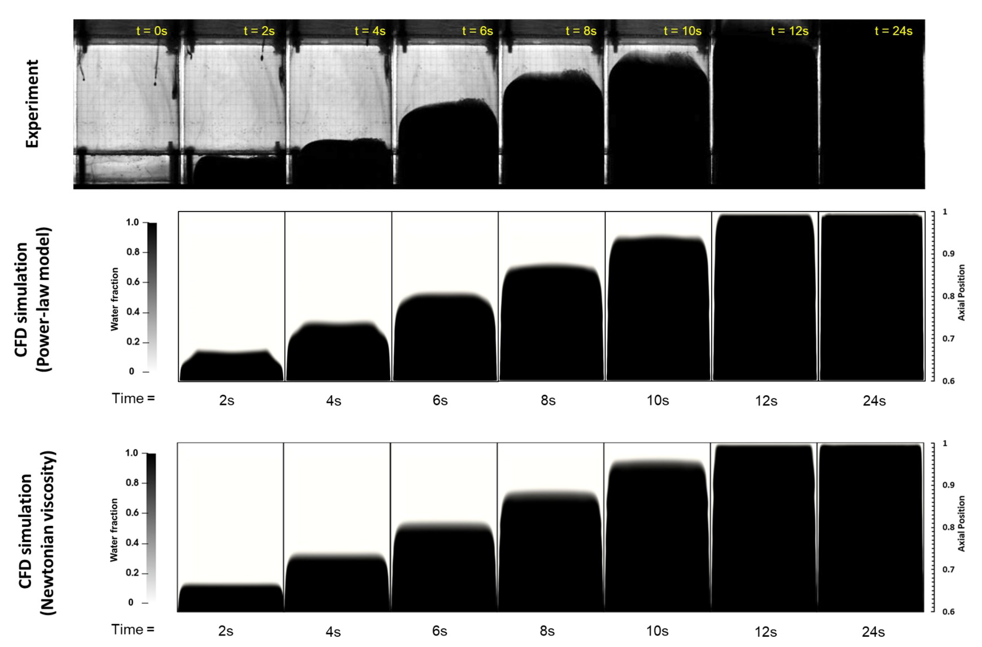
When comparing the results above from the different shear-thinning regimes, we note a significant impact of the displaced fluid viscosity on the displacement and the morphology of the fluid interface. It is obvious that the degree of shear-thinning significantly influences the development of interfacial patterns. In the weakly shear-thinning regime, the displacement of the interface is almost identical to that of displacement of a Newtonian fluid with an equivalent, effective viscosity as the original xanthan gum solution. Furthermore, no obvious viscous fingering patterns or other instabilities were identified.
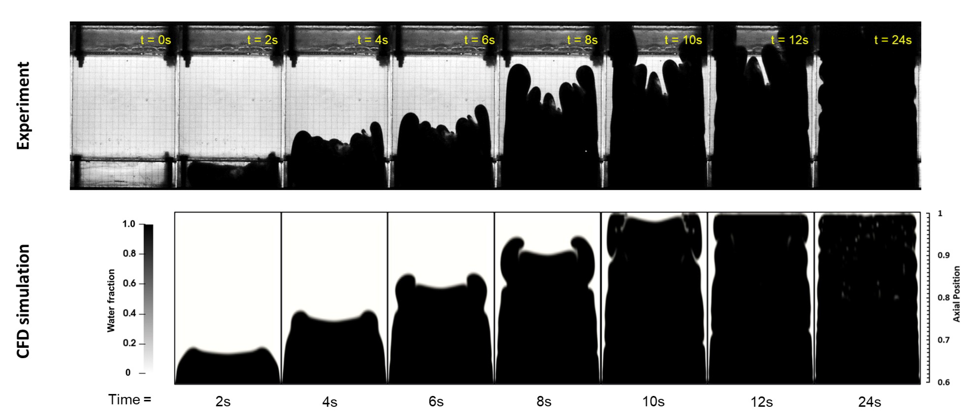
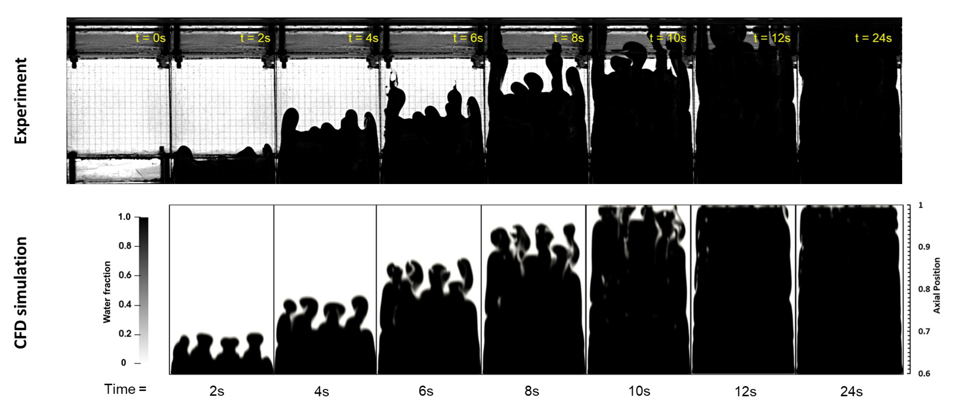
The moderate and strongly shear-thinning regimes both exhibited Saffman–Taylor type instability at the interface. In the moderately shear-thinning regime, several small finger-shaped channels formed across the interface, and the displaced fluid did not stagnate, possibly except for thin layers adjacent to the short side walls, as shown in Figure 6 and 
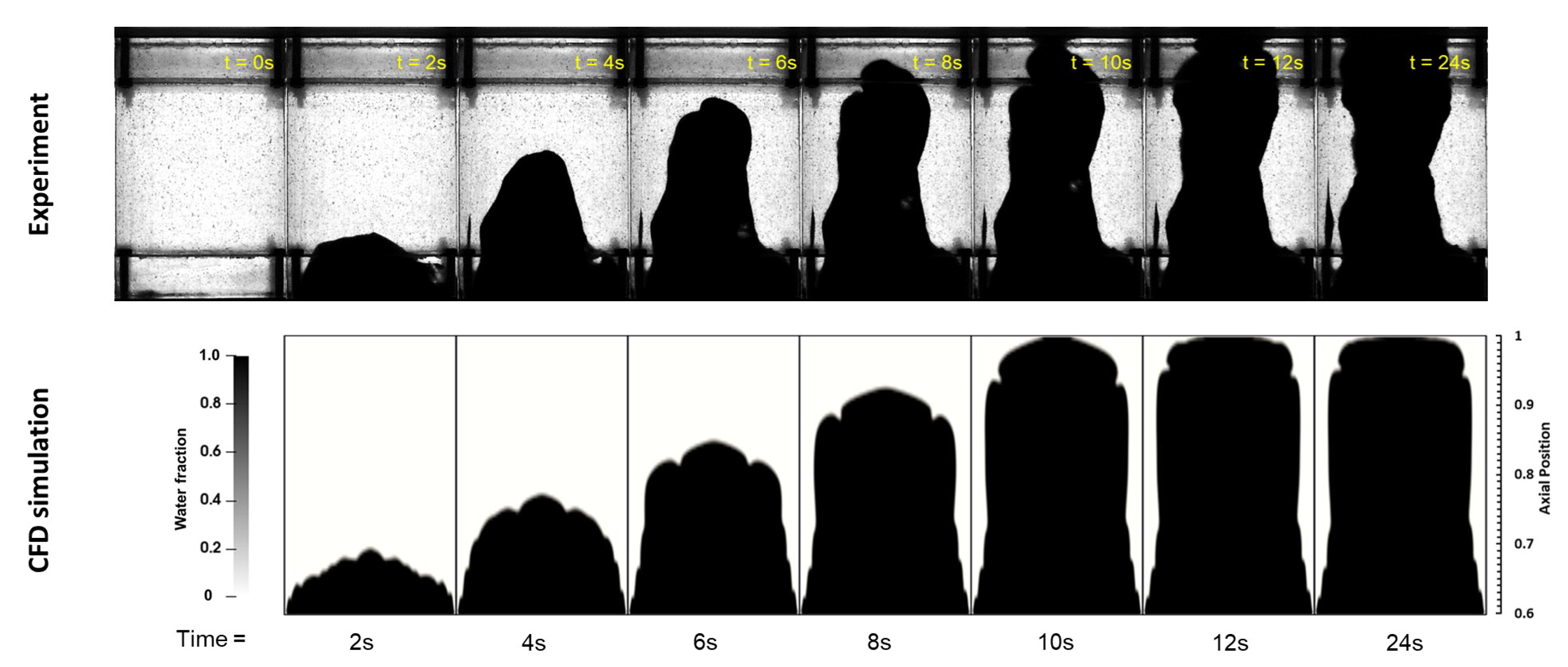
Figure 7. This allows the complete displacement of the shear-thinning fluid save for a relatively thin wall layer that displays a mild Kelvin–Helmholtz type of instability. In the strongly shear-thinning regime, the displacing fluid formed a unique channel through the displaced fluid. The displaced fluid appears to flow very slowly, if at all, on either side of the central channel. As a result, the displacing fluid accelerated through the relatively thin channel formed through the center of the duct and to the outlet. This created a relatively large wall layer and prevents the complete displacement of the duct.
We note that even if all xanthan gum solutions used for our experiments had effective viscosity greater than the displacing water, viscous fingering instabilities were only observed for the moderate and strongly shear-thinning regimes. We link this observation to the stabilizing effect of the density difference between the two fluids; as pointed out in the introduction, a density-stable fluid hierarchy will postpone the onset of viscous fingering. This is reasonable, since in a vertical channel, gravity acts to maintain a horizontal interface between the fluids. To assess the combined impact of gravity and viscosity on the stability of the displacements, we estimate and compare the “modified” pressure gradients for the (unperturbed) displaced and displacing fluid, G i = p i / z + ρ i g . The first term, p i / z , is taken as the fully developed, laminar pressure gradient of fluid i, and the second term is the hydrostatic component to the pressure gradient. As a first approximation, we use theoretical results for plane slot flow [40] for calculating the friction pressure gradient of the Newtonian and the power law fluids, i.e.,:
p z = κ 2 + 1 / n ( h / 2 ) 1 + 1 / n n U 0 n .
This is only considered an approximation since, in our experiments and simulations, the duct aspect ratio was only λ = W / h = 10 . As such, the side walls are expected to influence and reduce the volumetric flux for a given pressure differential. However, for the current discussion, we neglect the impact of the side walls and take Equation (5) as a coarse approximation to the pressure gradient in the different phases. Finally, for the displacing (Newtonian) fluid, the same equation applies by replacing n 1 and κ μ . The resulting, approximated pressure gradients for the fluids used in this study are listed in Table 3, along with the corresponding hydrostatic pressure gradient and the modified pressure gradient, G.
When comparing the pressure gradient of water with that of the shear-thinning solutions, we note that the modified pressure gradient of the displacing water exceeds that of the weakly shear-thinning fluid. As pointed out above, this case did not exhibit any viscous fingering instability in either experiment or numerical simulations. We attribute the lack of viscous fingers to the stabilizing effect of the density difference between the fluids, which is reflected in the modified pressure gradient of these fluids. In the other two cases, the friction pressure gradient associated with the moderate and highly shear-thinning fluids exceed the stabilizing hydrostatic component. This makes the modified pressure gradient larger in the displaced phase, as shown in Table 3. These two cases exhibited finger instabilities, both experimentally and in numerical simulations. Consequently, we find that our observations are consistent with a stability criterion based on the modified pressure gradients of the two fluids, similar to the classic Newtonian result [14].

5. Summary and Conclusions

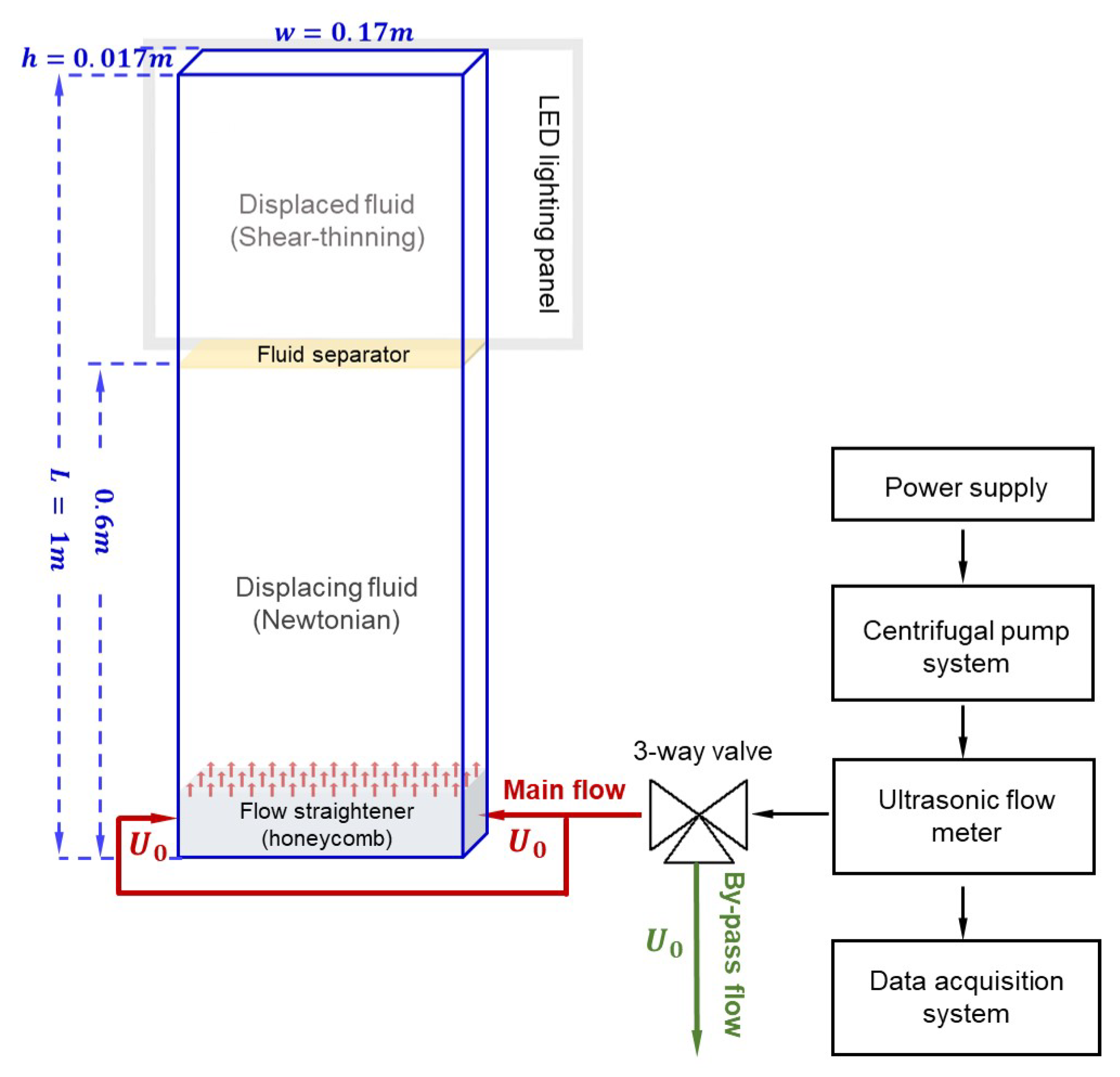
We have studied the displacement of different shear-thinning fluids by a denser but less viscous Newtonian fluid in a vertical, rectangular duct. Both experiments and fully three-dimensional numerical simulations have been performed to study the displacements, and with a particular focus on the interfacial region between the fluids and the growth of instabilities. A relatively small density difference was introduced to both examine the stabilizing effect of a positive density contrast, and also to improve repeatability of the experiments by maintaining a density-stable hierarchy at the start of the experiment. All displacement experiments and simulations were performed by imposed a fixed flow rate. We observed that the shape of the interface changed significantly as the displaced fluid was made more viscous and shear-thinning. As a result, our experiments and simulations were categorized as weakly, moderately and highly shear-thinning regimes.
The displacement in the weakly shear-thinning regime was found to be qualitatively similar to the displacement of a constant-viscosity Newtonian fluid. No obvious viscous finger formation was observed at the interface, and the displacement appeared stable, even if the fluid hierarchy was considerably viscosity-unstable. The lack of instabilities was attributed to the stabilizing effect on the interface by the density difference between the fluids. In the moderately shear-thinning regime, the displacing fluid formed several finger-shaped channels across the width of the duct. The finger structures are likely linked to the Saffman–Taylor instability, i.e., driven by the difference in viscosity of the two fluids. The displacement of shear-thinning fluid was relatively complete in this regime, leaving behind only a thin, residual wall layer. Finally, in the strongly shear-thinning regime, a central finger penetrated the displaced fluid and left behind considerable residual volume of non-displaced fluid on either side of this core.
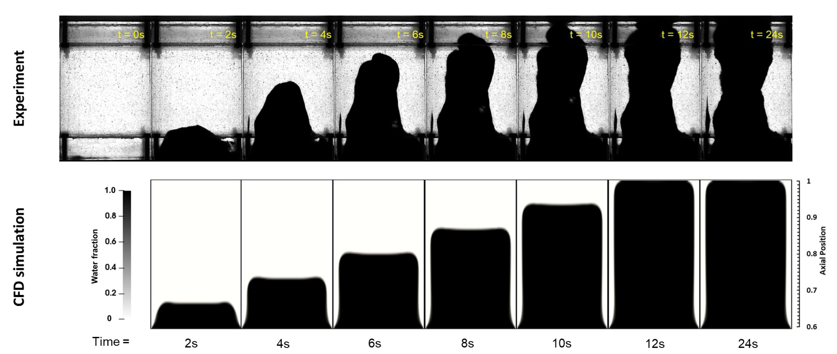
Numerical simulations have been performed using OpenFOAM, and the results compared to experimental observation for all three regimes. Simulation results and experiments are generally found to be in reasonable agreement for all three regimes. By introducing initial perturbations to the fluid interface in the numerical simulations, we observe improved agreement to the experimental results. This further suggests that the experimentally observed fingering and interface instability is indeed caused by a Saffman–Taylor type instability. Since the displaced fluid in our study is shear-thinning, the local fluid viscosity varies across the gap of the duct. Instead of linking the onset of viscous fingering instability to a specific, effective viscosity value, we instead interpret our observations in terms of the unperturbed pressure gradient within the displaced and displacing fluid phases. When accounting for the stabilizing density difference, we find that the pressure gradient is effective in predicting whether the displacement will be stable or not. This is found to be in accordance with theoretical linear stability analysis involving generalized Newtonian fluids [23].
As pointed out above, an important observation of the current study is that the onset of displacement instability appears linked to the pressure gradient in the two fluids. This observation is also in agreement with, e.g., design rules for effective laminar displacement, where the pressure gradient within the displacing fluid should be greater than that of the displaced fluid [16]. While the majority of past studies of the viscous fingering instability involves immiscible fluids, such as air displacing water or oil, the current study involves fluid configurations that are arguably more relevant for well construction, cementing and remediation operations.
Different interface dynamics from different shear-thinning regimes are visualized with experiments. We toned and bench marked a CFD tool that allows to generate dataset from computational experiments. With the aid of the toned computational tool, the cost of setting up experiments can be largely reduced, a wider range of displacement conditions can be investigated, and all relevant parameters can be easily altered. Thus, a more in-depth study of shear-thinning fluid displacement can be explored. Future studies will focus on in-depth analysis of the instability limit at the liquid interface for shear-thinning and other non-Newtonian fluid with data generated from the benchmarked CFD model. The selection criteria for finger-formation, and how this is linked to duct geometry and viscosity hierarchy will be explored.

Author Contributions

Conceptualization, Y.Z. and H.J.S.; methodology, Y.Z. and H.J.S.; investigation (experimental), Y.Z. and A.H.R.; investigation (computational), Y.Z.; formal analysis, Y.Z. and H.J.S.; data curation, Y.Z.; writing—original draft preparation, Y.Z.; writing—review and editing, H.J.S.; visualization, Y.Z.; supervision, H.J.S. All authors have read and agreed to the published version of the manuscript.

Funding

This research received no external funding.

Data Availability Statement

All data generated during this study are included in this published article.

Conflicts of Interest

The authors declare no conflict of interest.

References

  1. Hirasaki, G.; Pope, G. Analysis of Factors Influencing Mobility and Adsorption in the Flow of Polymer Solution Through Porous Media. Soc. Pet. Eng. J. 1974, 14, 337–346. Available online: https://onepetro.org/spejournal/article-pdf/14/04/337/2157055/spe-4026-pa.pdf (accessed on 30 November 2022). [CrossRef]
  2. Abidin, A.; Puspasari, T.; Nugroho, W. Polymers for Enhanced Oil Recovery Technology. Procedia Chem. 2012, 4, 11–16. [Google Scholar] [CrossRef] [Green Version]
  3. Henningsson, M.; Regner, M.; Östergren, K.; Trägårdh, C.; Dejmek, P. CFD simulation and ERT visualization of the displacement of yoghurt by water on industrial scale. J. Food Eng. 2007, 80, 166–175. [Google Scholar] [CrossRef]
  4. Orr, F., Jr.; Taber, J. Use of carbon dioxide in enhanced oil recovery. Science 1984, 224, 563–569. [Google Scholar] [CrossRef] [PubMed]
  5. Bittleston, S.; Ferguson, J.; Frigaard, I. Mud removal and cement placement during primary cementing of an oil well–Laminar non-Newtonian displacements in an eccentric annular Hele-Shaw cell. J. Eng. Math. 2002, 43, 229–253. [Google Scholar] [CrossRef]
  6. Sorensen, T.S. Dynamics and Instability of Fluid Interfaces; Springer: Berlin, Germany, 1979; Volume 105. [Google Scholar]
  7. Manikantan, H.; Squires, T.M. Surfactant dynamics: Hidden variables controlling fluid flows. J. Fluid Mech. 2020, 892, P1. [Google Scholar] [CrossRef]
  8. Rajan, G.K. Damping rate measurements and predictions for gravity waves in an air–oil–water system. Phys. Fluids 2022, 34, 022113. [Google Scholar] [CrossRef]
  9. Martyushev, L.; Bando, R.; Chervontseva, E. Instability of the fluid interface at arbitrary perturbation amplitudes. Displacement in the Hele–Shaw cell. Phys. A Stat. Mech. Appl. 2021, 562, 125391. [Google Scholar] [CrossRef]
  10. Lou, W.; Wang, Z.; Pan, S.; Sun, B.; Zhang, J.; Chen, W. Prediction model and energy dissipation analysis of Taylor bubble rise velocity in yield stress fluid. Chem. Eng. J. 2020, 396, 125261. [Google Scholar] [CrossRef]
  11. Saffman, P.G.; Taylor, G.I. The penetration of a fluid into a porous medium or Hele-Shaw cell containing a more viscous liquid. Proc. R. Soc. Lond. A 1958, 245, 312–329. [Google Scholar] [CrossRef]
  12. Homsy, G.M. Viscous Fingering in Porous Media. Annu. Rev. Fluid Mech. 1987, 19, 271–311. [Google Scholar] [CrossRef]
  13. Wilson, S.D.R. The Taylor–Saffman problem for a non-Newtonian liquid. J. Fluid Mech. 1990, 220, 413–425. [Google Scholar] [CrossRef]
  14. Leal, L. Advanced Transport Phenomena: Fluid Mechanics and Convective Transport Processes; Cambridge Series in Chemical Engineering; Cambridge University Press: Cambridge, UK, 2007. [Google Scholar]
  15. Mahardika, M.A.; She, Y.; Koe, T.; Patmonoaji, A.; Nasir, M.; Matshushita, S.; Suekane, T. Competition of gravity and viscous forces in miscible vertical displacement in a three-dimensional porous medium. Phys. Fluids 2022, 34, 073102. [Google Scholar] [CrossRef]
  16. Théron, B.E.; Bodin, D.; Fleming, J. Optimization of Spacer Rheology Using Neural Network Technology. In Proceedings of the SPE/IADC Drilling Conference and Exhibition, SPE-74498-MS, Dallas, TX, USA, 26–28 February 2002. [Google Scholar] [CrossRef]
  17. Carrasco-Teja, M.; Frigaard, I.A.; Seymour, B.R.; Storey, S. Viscoplastic fluid displacements in horizontal narrow eccentric annuli: Stratification and travelling wave solutions. J. Fluid Mech. 2008, 605, 293–327. [Google Scholar] [CrossRef]
  18. McCloud, K.V.; Maher, J.V. Experimental perturbations to Saffman–Taylor flow. Phys. Rep. 1995, 260, 139–185. [Google Scholar] [CrossRef]
  19. Lajeunesse, E.; Martin, J.; Rakotomalala, N.; Salin, D.; Yortsos, Y.C. Miscible displacement in a Hele-Shaw cell at high rates. J. Fluid Mech. 1999, 398, 299–319. [Google Scholar] [CrossRef] [Green Version]
  20. Fernandez, J.; Kurowski, P.; Petitjeans, P.; Meiburg, E. Density-driven unstable flows of miscible fluids in a Hele-Shaw cell. J. Fluid Mech. 2002, 451, 239–260. [Google Scholar] [CrossRef] [Green Version]
  21. Haudin, F.; Riolfo, L.A.; Knaepen, B.; Homsy, G.M.; De Wit, A. Experimental study of a buoyancy-driven instability of a miscible horizontal displacement in a Hele-Shaw cell. Phys. Fluids 2014, 26, 044102. [Google Scholar] [CrossRef] [Green Version]
  22. An, B.; Solorzano, D.; Yuan, Q. Viscous Fingering Dynamics and Flow Regimes of Miscible Displacements in a Sealed Hele-Shaw Cell. Energies 2022, 15, 5798. [Google Scholar] [CrossRef]
  23. Mora, S.; Manna, M. Saffman–Taylor instability for generalized Newtonian fluids. Phys. Rev. E 2009, 80, 016308. [Google Scholar] [CrossRef] [PubMed]
  24. Mora, S.; Manna, M. Saffman–Taylor instability of viscoelastic fluids: From viscous fingering to elastic fractures. Phys. Rev. E 2010, 81, 026305. [Google Scholar] [CrossRef] [PubMed]
  25. Lindner, A.; Bonn, D.; Poire, E.C.; Amar, M.B.; Meunier, J. Viscous fingering in non-Newtonian fluids. J. Fluid Mech. 2002, 469, 237–256. [Google Scholar] [CrossRef]
  26. Varges, P.R.; Azevedo, P.E.; Fonseca, B.S.; de Souza Mendes, P.R.; Naccache, M.F.; Martins, A.L. Immiscible liquid-liquid displacement flows in a Hele-Shaw cell including shear thinning effects. Phys. Fluids 2020, 32, 013105. [Google Scholar] [CrossRef]
  27. Jangir, P.; Mohan, R.; Chokshi, P. Experimental sutdy on the role of polymer addition in Saffman–Taylor instability in miscible flow displacement. Phys. Fluids 2022, 34, 093102. [Google Scholar] [CrossRef]
  28. Lindner, A.; Bonn, D.; Amar, M.B.; Meunier, J.; Kellay, H. Controlling viscous fingering. Europhys. News 1999, 30, 77–78. [Google Scholar] [CrossRef]
  29. Bonn, D.; Kellay, H.; Amar, M.B.; Meunier, J. Viscous finger widening with surfactants and polymers. Phys. Rev. Lett. 1995, 75, 2132. [Google Scholar] [CrossRef]
  30. Ahmadikhamsi, S.; Golfier, F.; Oltean, C.; Lefèvre, E.; Bahrani, S.A. Impact of surfactant addition on non-Newtonian fluid behavior during viscous fingering in Hele-Shaw cell. Phys. Fluids 2020, 32, 012103. [Google Scholar] [CrossRef]
  31. Barakat, J.M.; Squires, T.M. Curvature-Mediated Forces on Elastic Inclusions in Fluid Interfaces. Langmuir 2022, 38, 1099–1105. [Google Scholar] [CrossRef]
  32. Elfring, G.J.; Leal, L.G.; Squires, T.M. Surface viscosity and Marangoni stresses at surfactant laden interfaces. J. Fluid Mech. 2016, 792, 712–739. [Google Scholar] [CrossRef]
  33. Guzmán, E.; Maestro, A.; Carbone, C.; Ortega, F.; Rubio, R.G. Dilational Rheology of Fluid/Fluid Interfaces: Foundations and Tools. Fluids 2022, 7, 335. [Google Scholar] [CrossRef]
  34. Ballard, N.; Law, A.D.; Bon, S.A. Colloidal particles at fluid interfaces: Behaviour of isolated particles. Soft Matter 2019, 15, 1186–1199. [Google Scholar] [CrossRef] [PubMed]
  35. Mrokowska, M.M.; Krztoń-Maziopa, A. Viscoelastic and shear-thinning effects of aqueous exopolymer solution on disk and sphere settling. Sci. Rep. 2019, 9, 1–13. [Google Scholar] [CrossRef] [PubMed] [Green Version]
  36. Whitcomb, P.J.; Macosko, C.W. Rheology of Xanthan Gum. J. Rheol. 1978, 22, 493–505. [Google Scholar] [CrossRef]
  37. Metzner, A.B.; Reed, J.C. Flow of Non-Newtonian Fluids - Correlation of the Laminar, Transition, and Turbulent-flow Regions. AIChE J. 1955, 1, 434–440. [Google Scholar] [CrossRef]
  38. Roenby, J.; Bredmose, H.; Jasak, H. A computational method for sharp interface advection. R. Soc. Open Sci. 2016, 3, 160405. [Google Scholar] [CrossRef] [Green Version]
  39. Greenshields, C. OpenFOAM v6 User Guide: 7.3 Transport/Rheology Models; CFD Direct: Reading, UK, 2018. [Google Scholar]
  40. Kelessidis, V.; Maglione, R.; Tsamantaki, C.; Aspirtakis, Y. Optimal determination of rheological parameters for Herschel–Bulkley drilling fluids and impact on pressure drop, velocity profiles and penetration rates during drilling. J. Pet. Sci. Eng. 2006, 53, 203–224. [Google Scholar] [CrossRef]
Figure 1. Schematic of the experimental setup.
Fluids 08 00035 g001
Figure 2. Convergence and mesh independence study.
Fluids 08 00035 g002
Figure 3. The mesh grids used for CFD simulations.
Fluids 08 00035 g003
Figure 4. Experimental visualization (top) and CFD simulation (bottom) of interface evolution of water displacing 0.225 wt.% xanthan solution.
Fluids 08 00035 g004
Figure 5. Experimental visualization (top) and CFD simulations (bottom) of interface evolution of water displacing 0.02 wt.% xanthan gum solution. The case is simulated with both power-law and effective Newtonian viscosity for comparison.
Fluids 08 00035 g005
Figure 6. Experimental visualization (top) and CFD simulation (bottom) of interface evolution of water displacing 0.075 wt.% xanthan gum solution.
Fluids 08 00035 g006
Figure 7. Updated CFD simulation (bottom) of interface evolution of water displacing 0.075 wt.% xanthan gum solution with an initially perturbed interface.
Fluids 08 00035 g007
Figure 8. Updated CFD simulation (bottom) of interface evolution of water displacing 0.225 wt.% xanthan gum solution with induced perturbations at the initial interface.
Fluids 08 00035 g008
Table 1. Viscosity parametrization for the displaced fluid with different concentration xanthan gum.
Concentration (wt %) κ (Pa·s n )n
0.020.0160.69
0.0750.0770.52
0.2251.830.22
Table 2. Dimensionless number relevant for the current study.
NumberNameDefinitionRange or Value
λ Duct aspect ratio W / h 10
R e Reynolds number ρ ¯ U 0 2 / τ * 0.3–32.3
A t Atwood number Δ ρ / 2 ρ ¯ 0.001
F r Froude number U 0 / A t g h 2.05
n 1 Shear-thinning index of fluid 1 n 1 0.2–0.7
MViscosity ratio μ 1 * / μ 2 14–1293
Table 3. Modified friction pressure gradient.
Liquid p / z (Pa/m) ρ g (Pa/m)G(Pa/m)
Water1.19810.09811.1
0.02 wt.% xanthan sol.9.69790.49800.0
0.075 wt.% xanthan sol.33.39790.49823.7
0.225 wt.% xanthan sol.412.49790.410,202.8
Disclaimer/Publisher’s Note: The statements, opinions and data contained in all publications are solely those of the individual author(s) and contributor(s) and not of MDPI and/or the editor(s). MDPI and/or the editor(s) disclaim responsibility for any injury to people or property resulting from any ideas, methods, instructions or products referred to in the content.

