
Navier–Stokes Equations and Bulk Viscosity for a Polyatomic Gas with Temperature-Dependent Specific Heats

Abstract
:1. Introduction
2. ES Model for a Gas with Temperature-Dependent Specific Heats
2.1. ES Model
2.2. Basic Properties
- Conservations: For an arbitrary function , the following relation holds:where () are , (), and for ; and () are , (), , and for .
- Equilibrium: The vanishing of the collision term is equivalent to the fact that f is the following local equilibrium distribution:for , where , , and are arbitrary functions of t and , and ; andfor , where , , , and are arbitrary functions of t and , and and are determined by the following coupled equations:The solution of (10) exists. In particular, it is unique when .
- Mean free path: The mean free path of the gas molecules in the equilibrium state at rest, at density , and temperature is given byfor the ES model (2), since is the collision frequency at this equilibrium state.
- Relaxation: In the space homogeneous case, where , the macroscopic quantities , , and T are constant, and the temperatures and relax to T in the following manner:where and are, respectively, the values of and at the initial time satisfying the relation with . Since is the mean free time, the time scale of relaxation of the temperatures is the mean free time devided by . Therefore, we may regard as the parameter controlling the speed of relaxation of the internal modes. This situation is the same as in the case of the ES model with constant [36].
3. Ordinary Navier–Stokes Equations with a Single Temperature
4. Navier–Stokes Equations with Two Temperatures
5. Some Remarks
6. Shock-Wave Structure
6.1. Problem
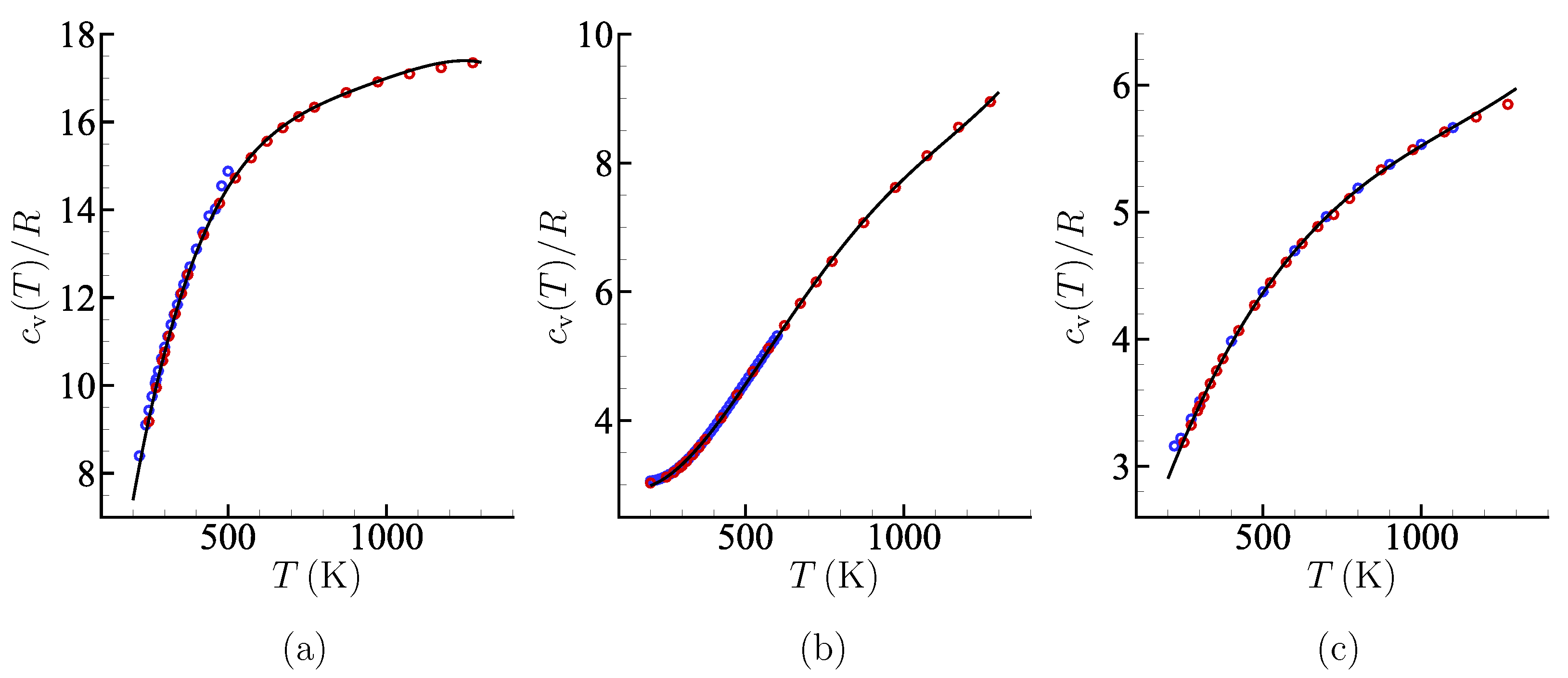
6.2. Properties of Some Gases with Large Bulk Viscosities
6.3. Numerical Results
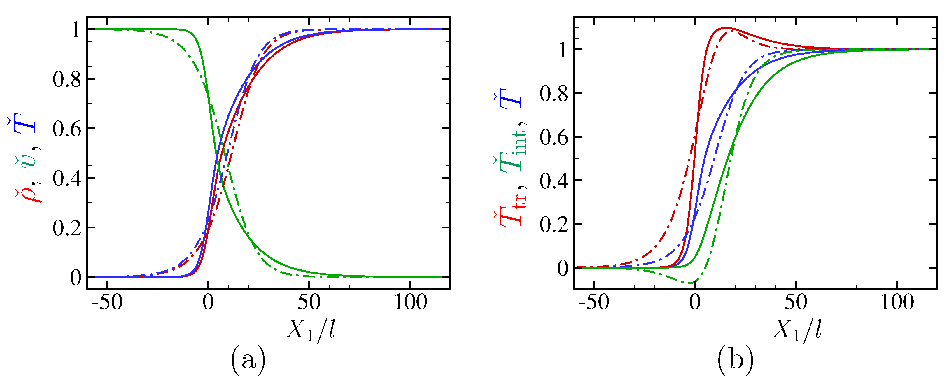
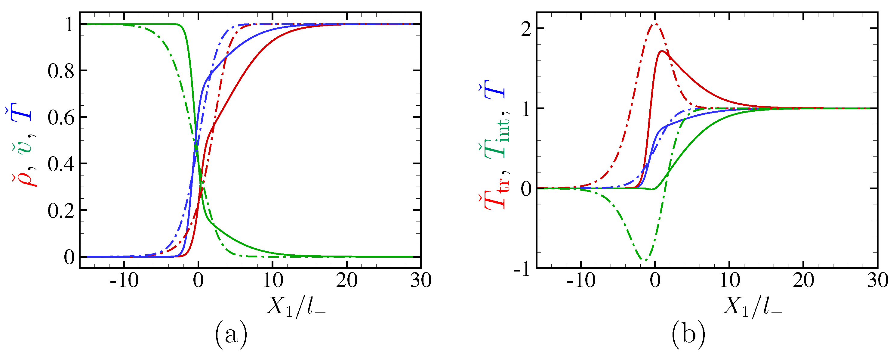
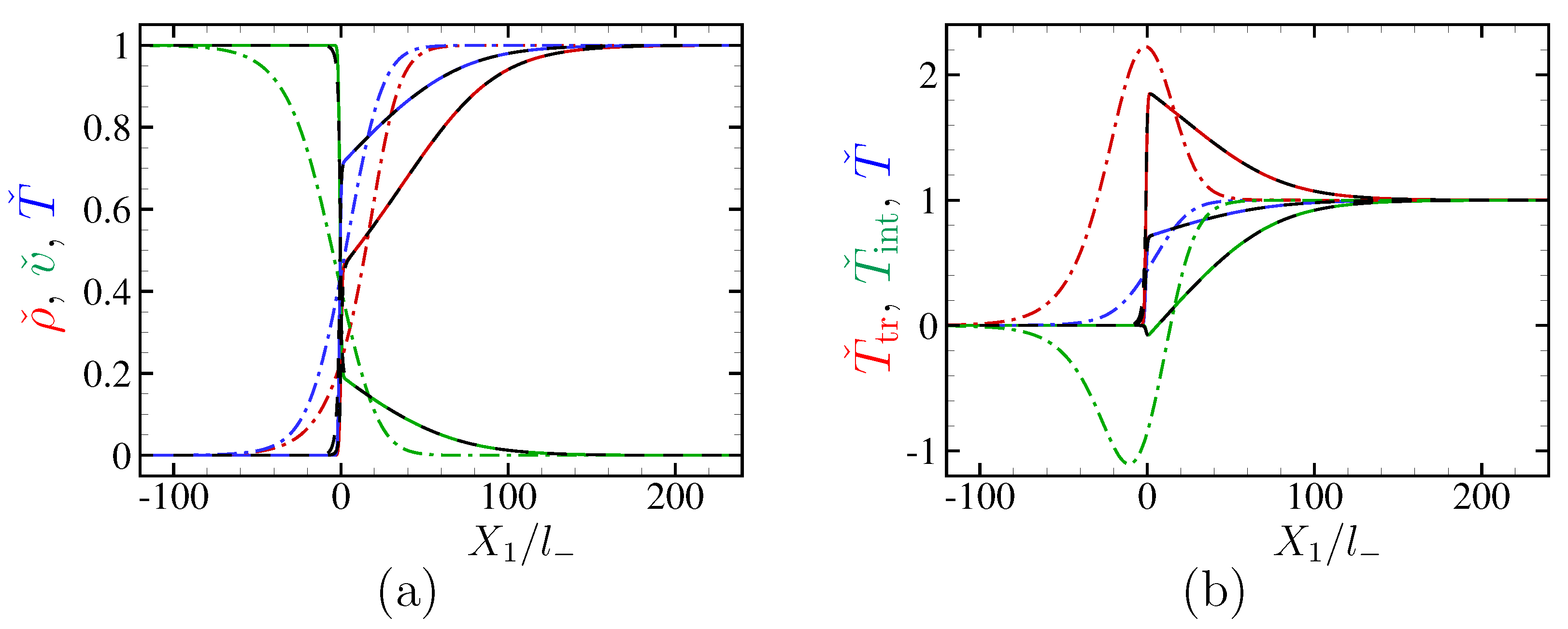
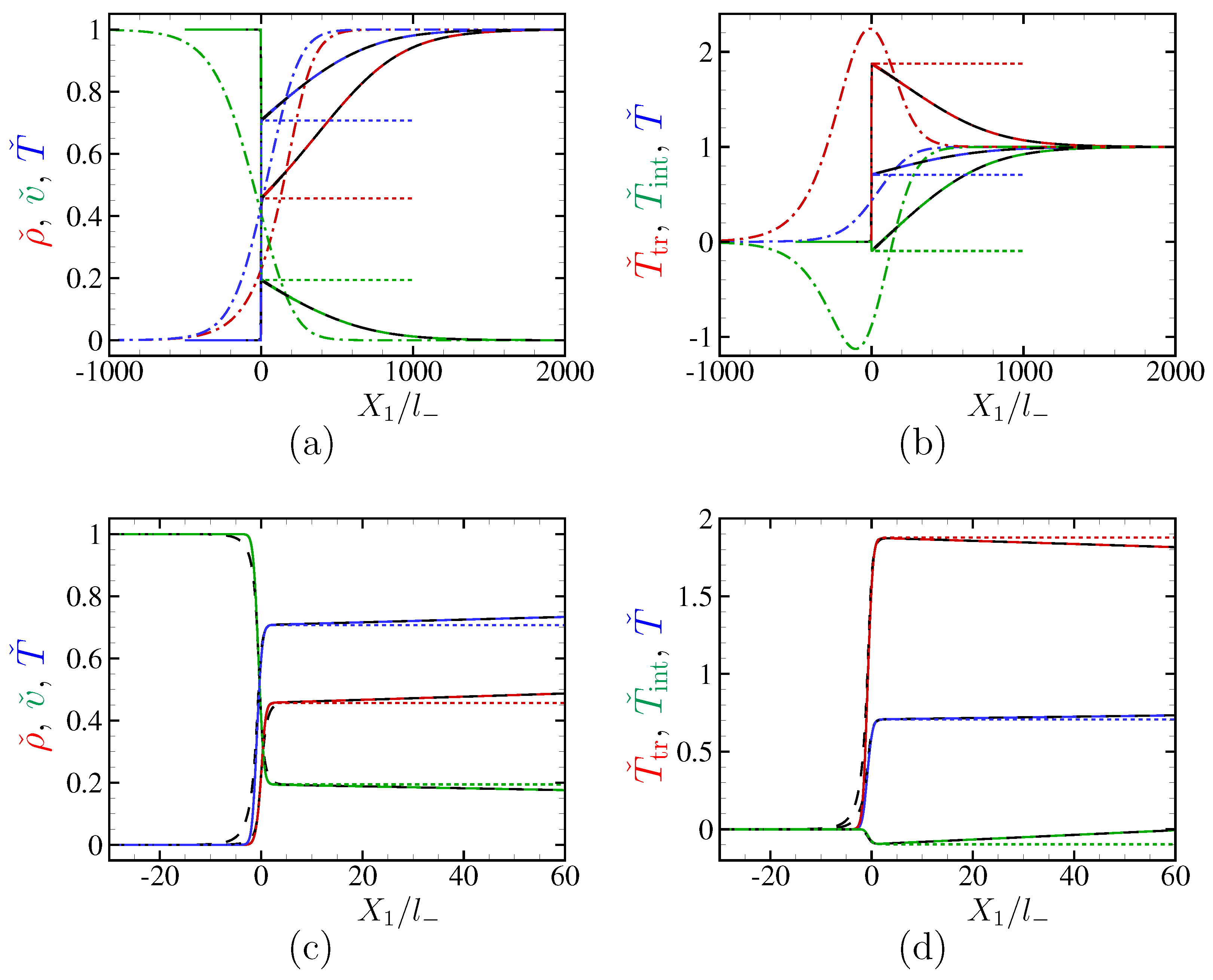
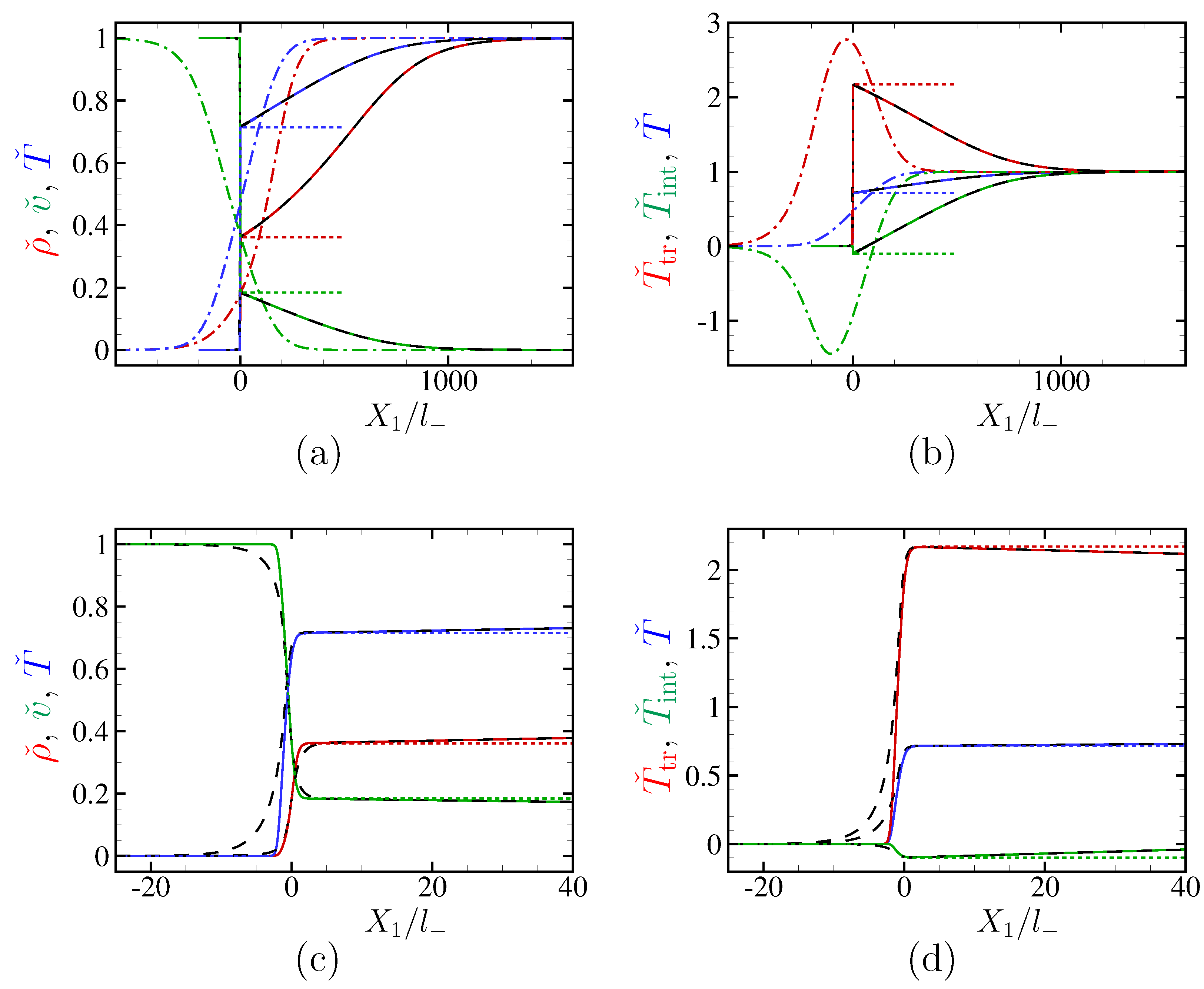
6.3.1. CO Gas
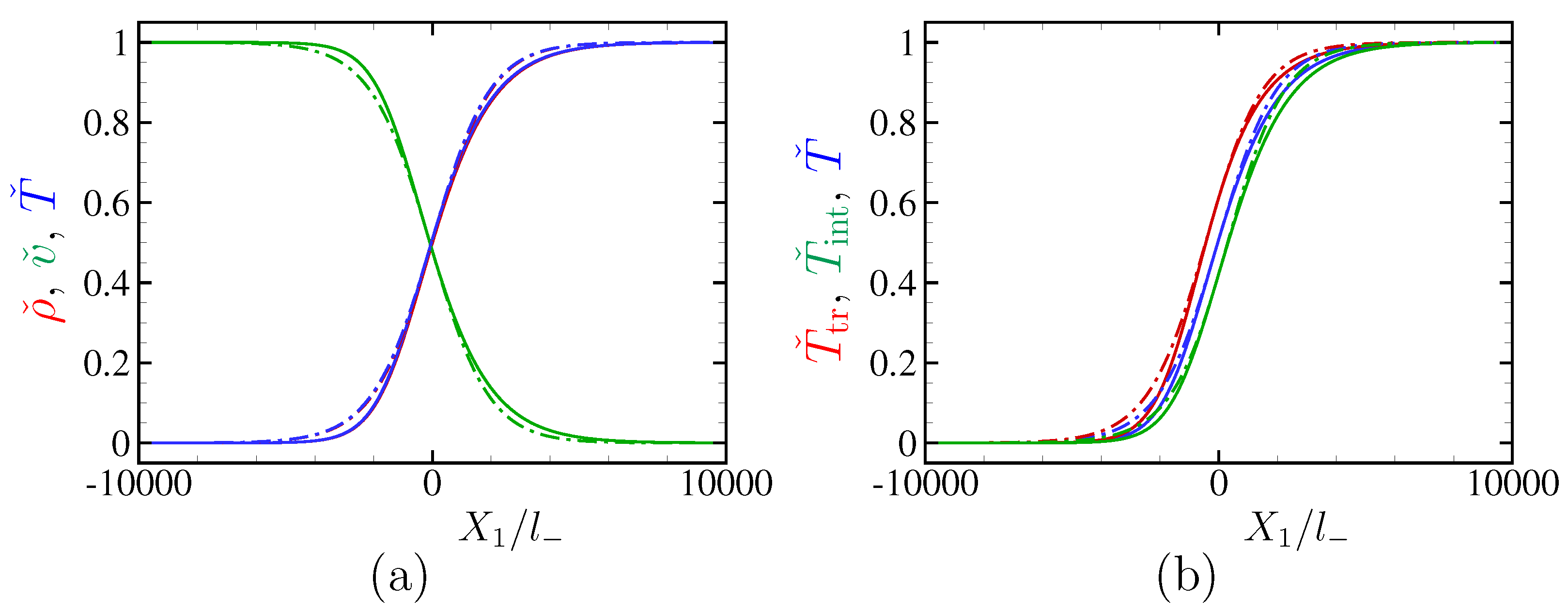
- (i)
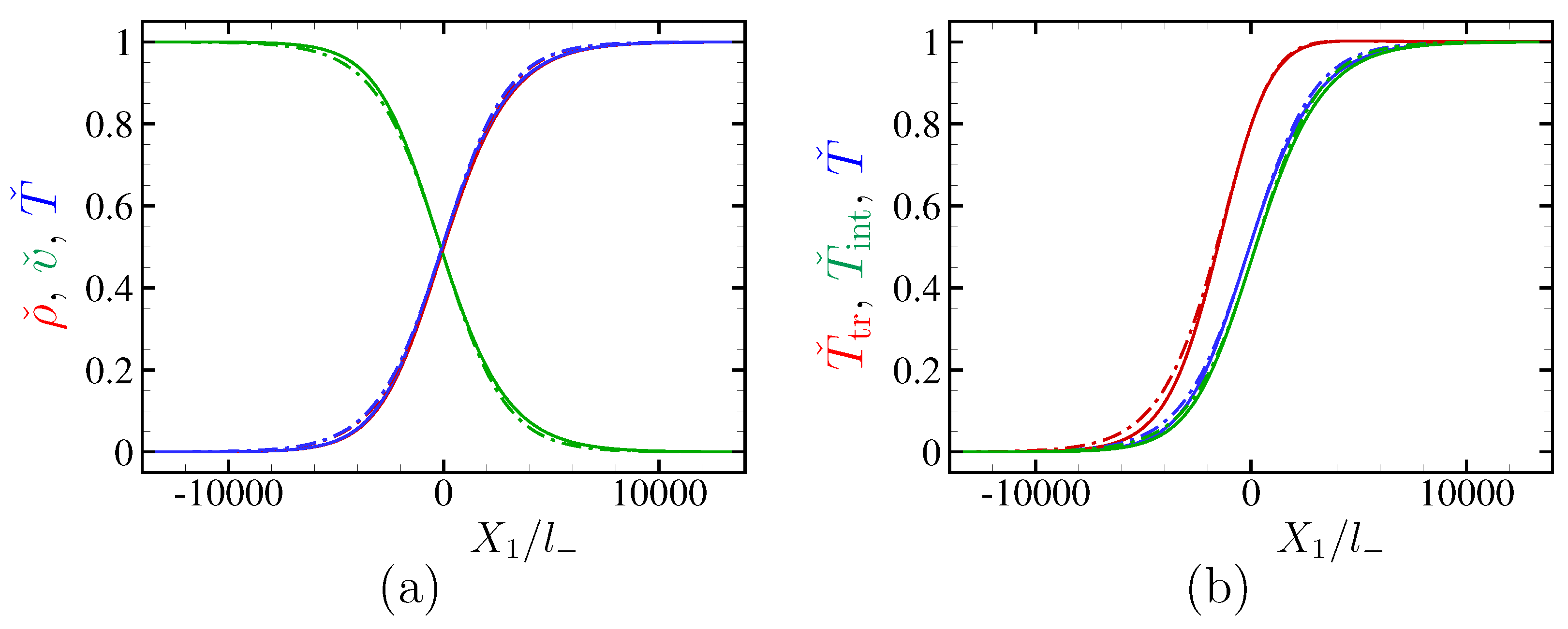
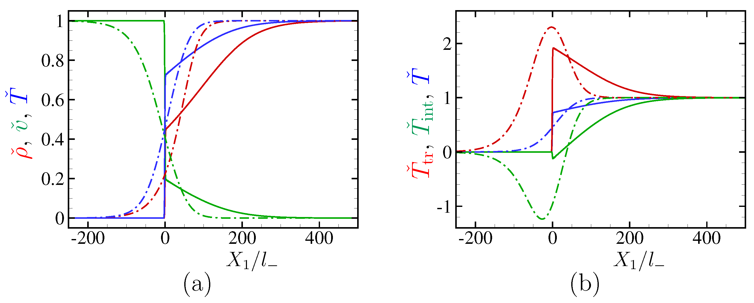
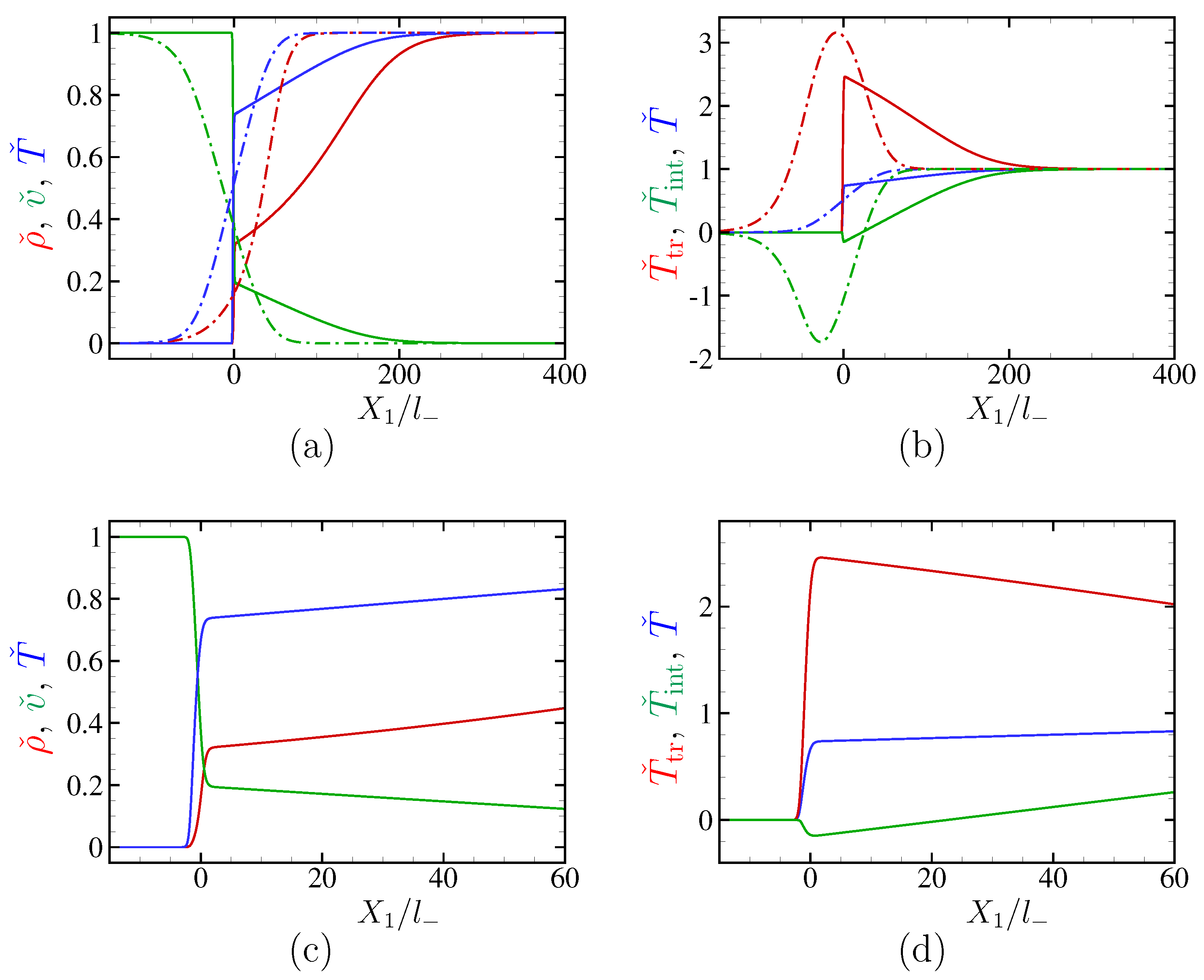
- The two-temperature NS equations are able to reproduce correct shock profiles for weak shock waves ().
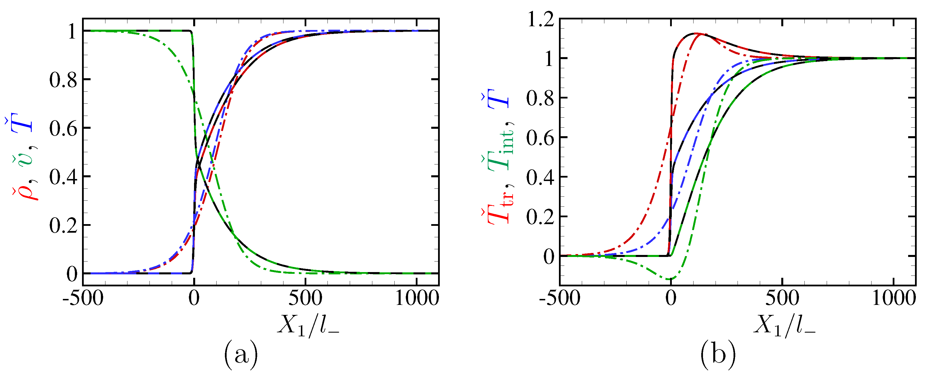
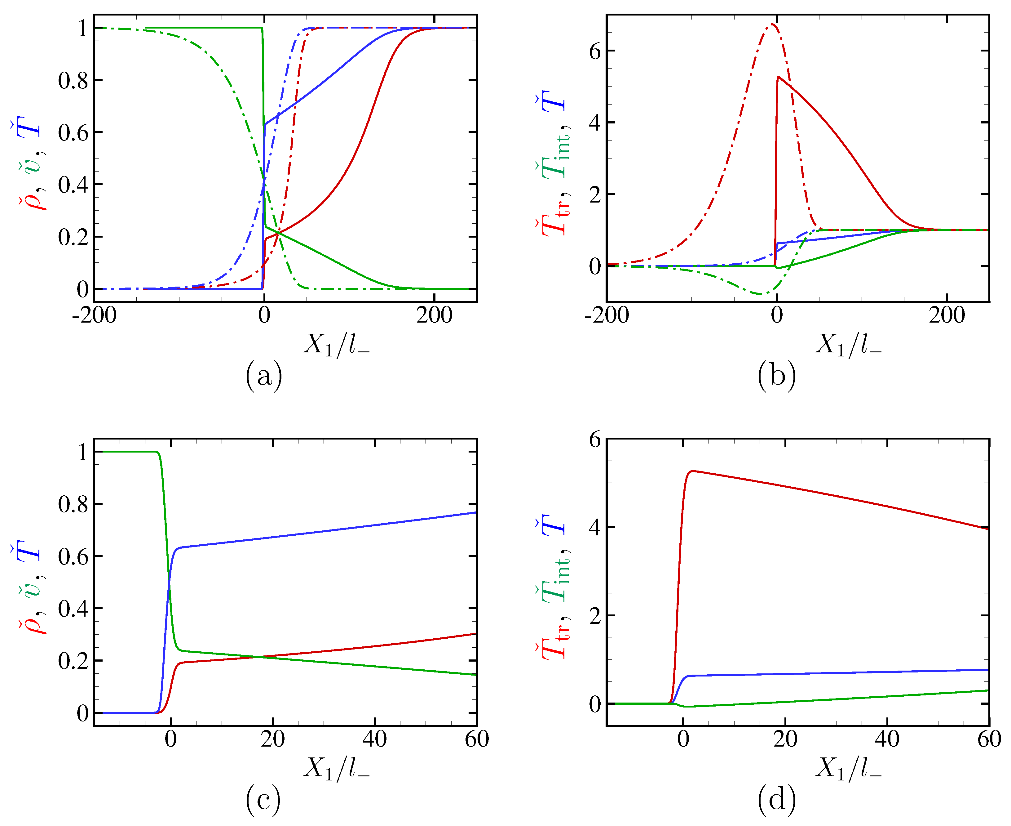
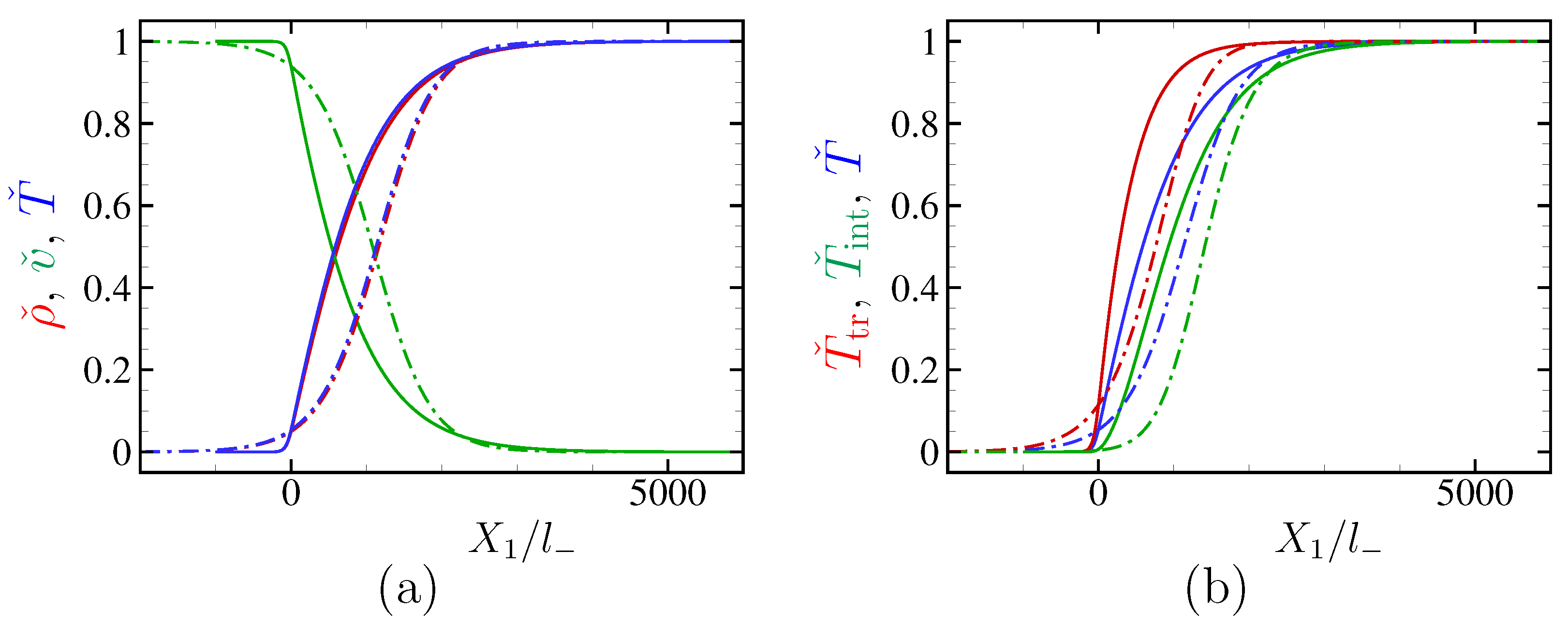
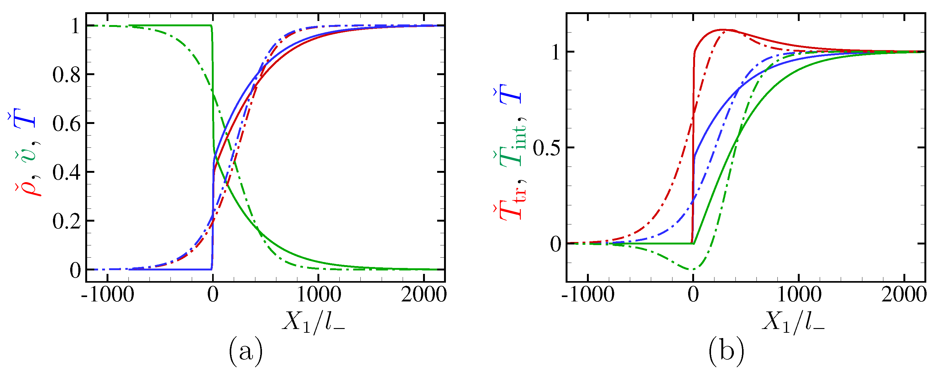
- (ii)
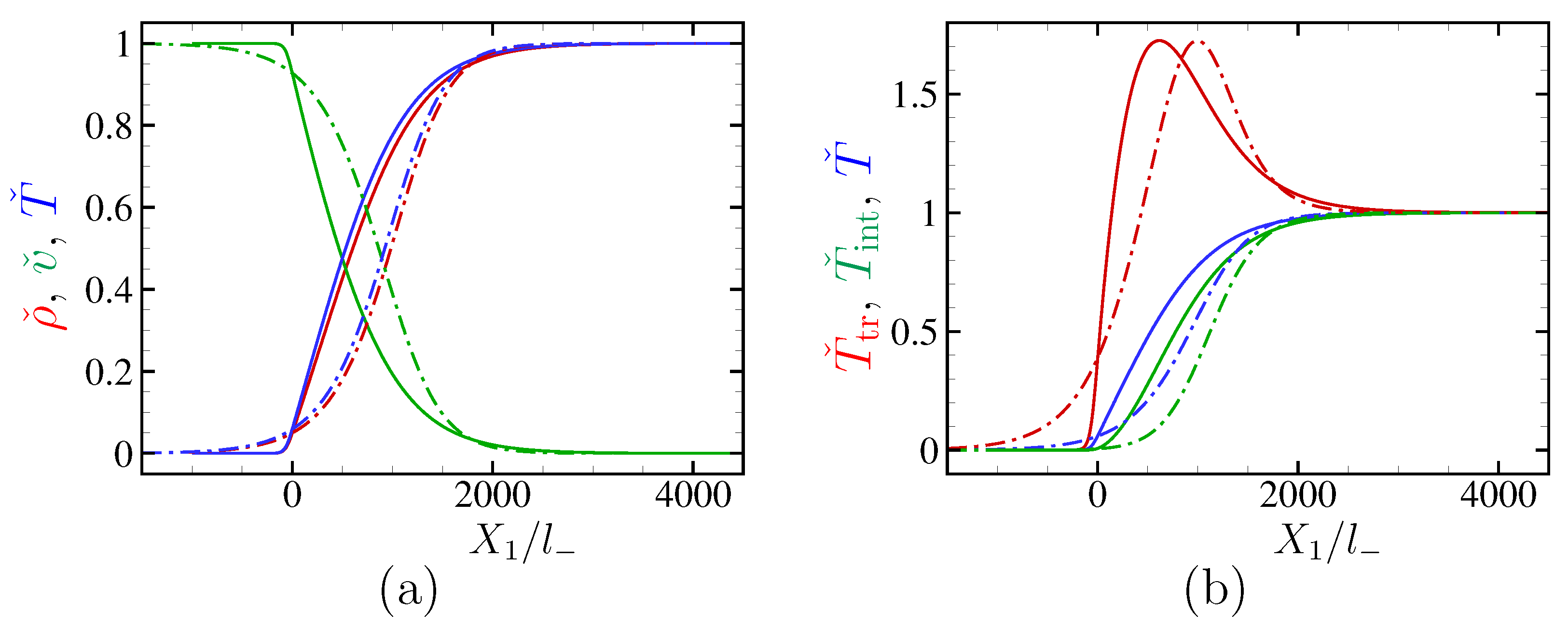
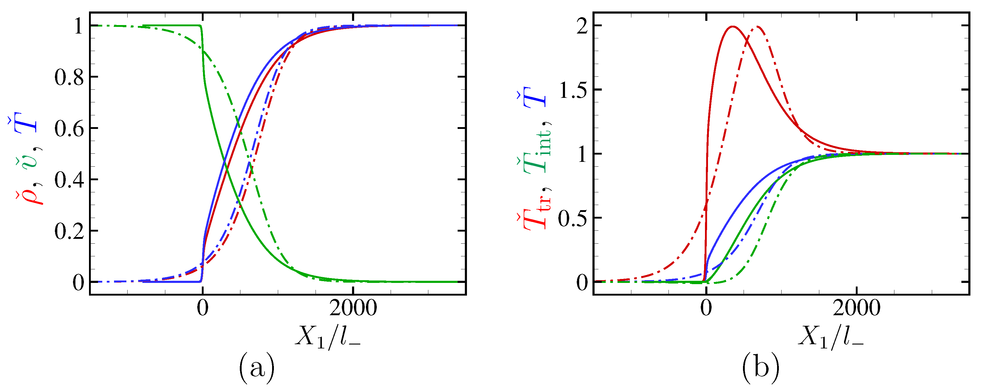
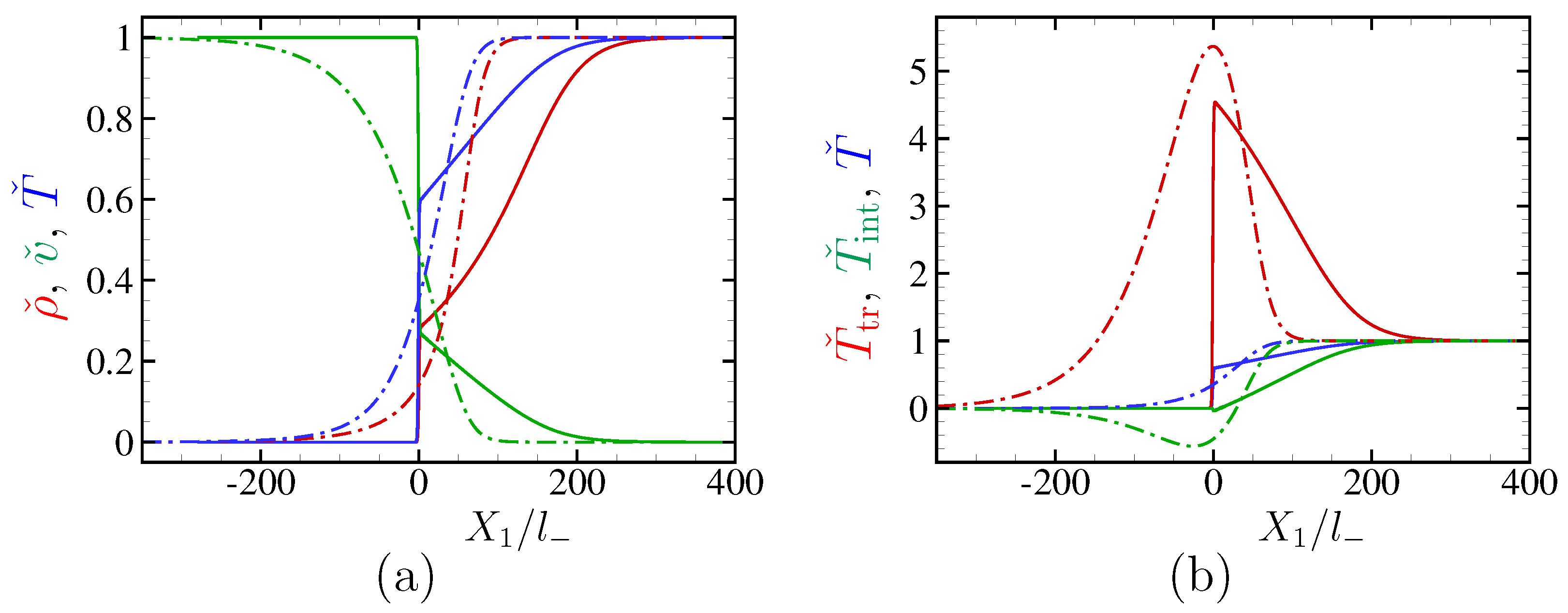
- For moderate and strong shock waves ( and 5), although the profiles obtained by the two-temperature NS equations deviate from those based on the ES model in the thin front layer (subshock), they agree very well in the thick rear layer. The two-temperature NS equations tend to give a thinner and sharper subshock.
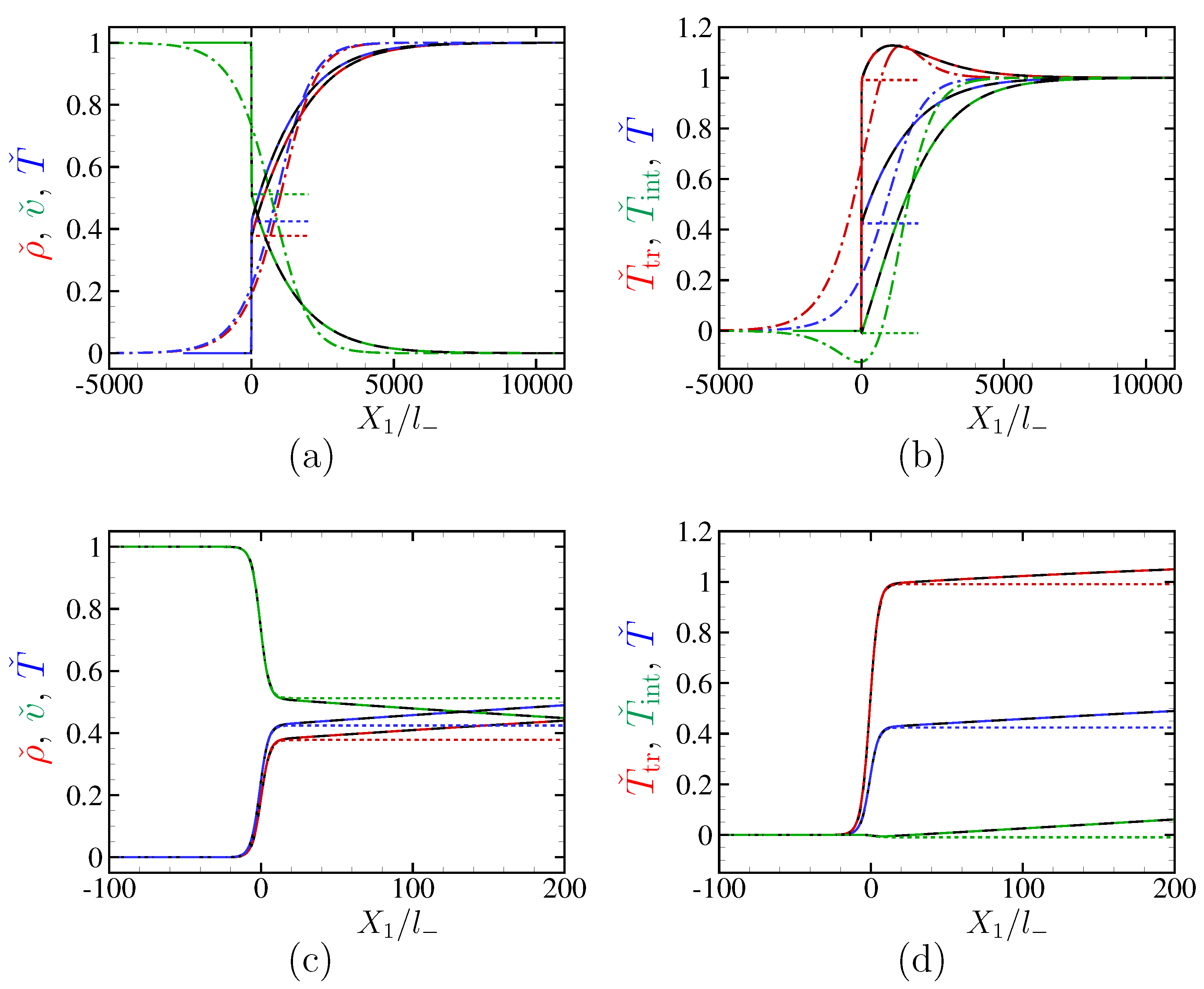
- (iii)
- The profiles of the subshock coincide with those of the shock wave with .
- (iv)
- The ordinary NS equations (with bulk viscosity) cannot be used to correctly describe the shock-wave structure even for weak shock waves ().
6.3.2. SF Gas
6.3.3. CH Gas
7. Concluding Remarks
Author Contributions
Funding
Institutional Review Board Statement
Informed Consent Statement
Data Availability Statement
Conflicts of Interest
References
- Anderson, J.D., Jr. Hypersonic and High Temperature Gas Dynamics; McGraw-Hill: New York, NY, USA, 1989. [Google Scholar]
- Park, C. Nonequilibrium Hypersonic Aerothermodynamics; John Wiley & Sons: New York, NY, USA, 1990. [Google Scholar]
- Nagnibeda, E.; Kustova, E. Non-Equilibrium Reacting Gas Flows: Kinetic Theory of Transport and Relaxation Processes; Springer: Berlin, Germany, 2009. [Google Scholar]
- Boyd, I.D.; Schwartzentruber, T.E. Nonequilibrium Gas Dynamics and Molecular Simulation; Cambridge University Press: Cambridge, UK, 2017. [Google Scholar]
- Wang Chang, C.S.; Uhlenbeck, G.E. Transport Phenomena in Polyatomic Gases; Engineering Research Institute Report CM-681; University of Michigan: Ann Arbor, MI, USA, 1951. [Google Scholar]
- Ferziger, J.H.; Kaper, H.G. Mathematical Theory of Transport Processes in Gases; North Holland: Amsterdam, The Netherlands, 1972. [Google Scholar]
- McCourt, F.R.W.; Beenakker, J.J.M.; Köhler, W.E.; Kuščer, I. Nonequilibrium Phenomena in Polyatomic Gases, Volume 1: Dilute Gases; Clarendon: Oxford, UK, 1990. [Google Scholar]
- Giovangigli, V. Multicomponent Flow Modeling; Birkhäuser: Boston, MA, USA, 1999. [Google Scholar]
- Borgnakke, C.; Larsen, P.S. Statistical collision model for Monte Carlo simulation of polyatomic gas mixture. J. Comp. Phys. 1975, 18, 405–420. [Google Scholar] [CrossRef]
- Bourgat, J.-F.; Desvillettes, L.; Le Tallec, P.; Perthame, B. Microreversible collisions for polyatomic gases and Boltzmann’s theorem. Eur. J. Mech. B Fluids 1994, 13, 237–254. [Google Scholar]
- Desvillettes, L.; Monaco, R.; Salvarani, F. A kinetic model allowing to obtain the energy law of polytropic gases in the presence of chemical reactions. Eur. J. Mech. B Fluids 2005, 24, 219–236. [Google Scholar] [CrossRef]
- Borsoni, T.; Bisi, M.; Groppi, M. A general framework for the kinetic modelling of polyatomic gases. Commun. Math. Phys. 2022, 393, 215–266. [Google Scholar] [CrossRef]
- Pavić-Čolić, M.; Simić, S. Kinetic description of polyatomic gases with temperature-dependent specific heats. Phys. Rev. Fluids 2022, 7, 083401. [Google Scholar] [CrossRef]
- Boudin, L.; Rossi, A.; Salvarani, F. A kinetic model of polyatomic gas with resonant collisions. Ricerche Mat. 2022. [Google Scholar] [CrossRef]
- Gamba, I.M.; Pavić-Čolić, M. On the Cauchy problem for Boltzmann equation modelling a polyatomic gas. arXiv Prepr. 2020, arXiv:2005.01017. [Google Scholar]
- Brull, S.; Shahine, M.; Thieullen, P. Compactness property of the linearized Boltzmann operator for a diatomic single gas model. Netw. Heterog. Media 2022, 17, 847–861. [Google Scholar] [CrossRef]
- Bernhoff, N. Linearized Boltzmann collision operator: II. Polyatomic molecules modeled by a continuous internal energy variable. arXiv Prepr. 2022, arXiv:2201.01377. [Google Scholar]
- Morse, T.F. Kinetic model for gases with internal degrees of freedom. Phys. Fluids 1964, 7, 159–169. [Google Scholar] [CrossRef]
- Holway, L.H., Jr. New statistical models for kinetic theory: Methods of construction. Phys. Fluids 1966, 9, 1658–1673. [Google Scholar] [CrossRef]
- Rykov, V.A. A model kinetic equation for a gas with rotational degrees of freedom. Fluid Dyn. 1975, 10, 959–966. [Google Scholar] [CrossRef]
- Andries, P.; Le Tallec, P.; Perlat, J.-P.; Perthame, B. The Gaussian-BGK model of Boltzmann equation with small Prandtl number. Eur. J. Mech. B Fluids 2000, 19, 813–830. [Google Scholar] [CrossRef]
- Brull, S.; Schneider, J. On the ellipsoidal statistical model for polyatomic gases. Contin. Mech. Thermodyn. 2009, 20, 489–508. [Google Scholar] [CrossRef] [Green Version]
- Rahimi, B.; Struchtrup, H. Capturing non-equilibrium phenomena in rarefied polyatomic gases: A high-order macroscopic model. Phys. Fluids 2014, 26, 052001. [Google Scholar] [CrossRef]
- Bisi, M.; Spiga, G. On kinetic models for polyatomic gases and their hydrodynamic limits. Ric. Mat. 2017, 66, 113–124. [Google Scholar] [CrossRef]
- Baranger, C.; Dauvois, Y.; Marois, G.; Mathé, J.; Mathiaud, J.; Mieussens, L. A BGK model for high temperature rarefied gas flows. Eur. J. Mech. B Fluids 2020, 80, 1–12. [Google Scholar] [CrossRef] [Green Version]
- Dauvois, Y.; Mathiaud, J.; Mieussens, L. An ES-BGK model for polyatomic gases in rotational and vibrational nonequilibrium. Eur. J. Mech. B Fluids 2021, 88, 1–16. [Google Scholar] [CrossRef]
- Mathiaud, J.; Mieussens, L.; Pfeiffer, M. An ES-BGK model for diatomic gases with correct relaxation rates for internal energies. Eur. J. Mech. B Fluids 2022, 96, 65–77. [Google Scholar] [CrossRef]
- Myong, R.S. Coupled nonlinear constitutive models for rarefied and microscale gas flows: Subtle interplay of kinematics and dissipation effects. Contin. Mech. Thermodyn. 2009, 21, 389–399. [Google Scholar] [CrossRef]
- Arima, T.; Taniguchi, S.; Ruggeri, T.; Sugiyama, M. Extended thermodynamics of real gases with dynamic pressure: An extension of Meixner’s theory. Phys. Lett. A 2012, 376, 2799–2803. [Google Scholar] [CrossRef]
- Pavić, M.; Ruggeri, T.; Simić, S. Maximum entropy principle for rarefied polyatomic gases. Phys. A 2013, 392, 1302–1317. [Google Scholar] [CrossRef] [Green Version]
- Taniguchi, S.; Arima, T.; Ruggeri, T.; Sugiyama, M. Overshoot of the non-equilibrium temperature in the shock wave structure of a rarefied polyatomic gas subject to the dynamic pressure. Int. J. Non-Linear Mech. 2016, 79, 66–75. [Google Scholar] [CrossRef]
- Arima, T.; Ruggeri, T.; Sugiyama, M. Rational extended thermodynamics of a rarefied polyatomic gas with molecular relaxation processes. Phys. Rev. E 2017, 96, 042143. [Google Scholar] [CrossRef] [Green Version]
- Pavić-Čolić, M.; Madjarević, D.; Simić, S. Polyatomic gases with dynamic pressure: Kinetic non-linear closure and the shock structure. Int. J. Non-Linear Mech. 2017, 92, 160–175. [Google Scholar] [CrossRef]
- Bisi, M.; Ruggeri, T.; Spiga, G. Dynamical pressure in a polyatomic gas: Interplay between kinetic theory and extended thermodynamics. Kin. Rel. Models 2018, 11, 71–95. [Google Scholar] [CrossRef] [Green Version]
- Ruggeri, T.; Sugiyama, M. Classical and Relativistic Rational Extended Thermodynamics of Gases; Springer: Cham, Switzerland, 2021. [Google Scholar]
- Aoki, K.; Bisi, M.; Groppi, M.; Kosuge, S. Two-temperature Navier–Stokes equations for a polyatomic gas derived from kinetic theory. Phys. Rev. E 2020, 102, 023104. [Google Scholar] [CrossRef]
- Chapman, S.; Cowling, T.G. The Mathematical Theory of Non-Uniform Gases, 3rd ed.; Cambridge University Press: Cambridge, UK, 1991. [Google Scholar]
- Grad, H. Principles of the kinetic theory of gases. In Handbuch der Physik; Band XII; Flügge, S., Ed.; Springer: Berlin, Germany, 1958; pp. 205–294. [Google Scholar]
- Cercignani, C. The Boltzmann Equation and Its Applications; Springer: Berlin, Germany, 1988. [Google Scholar]
- Sone, Y. Molecular Gas Dynamics: Theory, Techniques, and Applications; Birkhäuser: Boston, MA, USA, 2007; Supplementary Notes and Errata; Available online: http://hdl.handle.net/2433/66098 (accessed on 21 July 2019).
- Kosuge, S.; Kuo, H.-W.; Aoki, K. A kinetic model for a polyatomic gas with temperature-dependent specific heats and its application to shock-wave structure. J. Stat. Phys. 2019, 177, 209–251. [Google Scholar] [CrossRef]
- Park, C.; Yoon, S. Calculation of real-gas effects on blunt-body trim angles. AIAA J. 1992, 30, 999–1007. [Google Scholar] [CrossRef]
- Park, C.; Lee, S.-H. Validation of multitemperature nozzle flow code. J. Thermophys. Heat Trans. 1995, 9, 9–16. [Google Scholar] [CrossRef]
- Bruno, D.; Giovangigli, V. Relaxation of internal temperature and volume viscosity. Phys. Fluids 2011, 23, 093104, Erratum in Phys. Fluids 2013, 25, 039902. [Google Scholar] [CrossRef] [Green Version]
- Bruno, D.; Giovangigli, V. Internal energy relaxation processes and bulk viscosities in fluids. Fluids 2022, 7, 356. [Google Scholar] [CrossRef]
- Kosuge, S.; Aoki, K.; Bisi, M.; Groppi, M.; Martalò, G. Boundary conditions for two-temperature Navier–Stokes equations for a polyatomic gas. Phys. Rev. Fluids 2021, 6, 083401. [Google Scholar] [CrossRef]
- Bird, G.A. Molecular Gas Dynamics and the Direct Simulation of Gas Flows; Oxford University Press: Oxford, UK, 1994. [Google Scholar]
- Smiley, E.F.; Winkler, E.H.; Slawsky, Z.I. Measurement of the vibrational relaxation effect in CO2 by means of shock tube interferograms. J. Chem. Phys. 1952, 20, 923–924. [Google Scholar] [CrossRef]
- Smiley, E.F.; Winkler, E.H. Shock-tube measurements of vibrational relaxation. J. Chem. Phys. 1954, 22, 2018–2022. [Google Scholar] [CrossRef]
- Griffith, W.D.; Kenny, A. On fully-dispersed shock waves in carbon dioxide. J. Fluid Mech. 1957, 3, 286–289. [Google Scholar] [CrossRef]
- Johannesen, N.H.; Zienkiewicz, H.K.; Blythe, P.A.; Gerrard, J.H. Experimental and theoretical analysis of vibrational relaxation regions in carbon dioxide. J. Fluid Mech. 1962, 13, 213–225. [Google Scholar] [CrossRef]
- Taniguchi, S.; Arima, T.; Ruggeri, T.; Sugiyama, M. Effect of the dynamic pressure on the shock wave structure in a rarefied polyatomic gas. Phys. Fluids 2014, 26, 016103. [Google Scholar] [CrossRef]
- Taniguchi, S.; Arima, T.; Ruggeri, T.; Sugiyama, M. Thermodynamic theory of the shock wave structure in a rarefied polyatomic gas: Beyond the Bethe-Teller theory. Phys. Rev. E 2014, 89, 013025. [Google Scholar] [CrossRef]
- Alekseev, I.V.; Kosareva, A.A.; Kustova, E.V.; Nagnibeda, E.A. Various continuum approaches for studying shock wave structure in carbon dioxide. In Proceedings of the The Eighth Polyakhov’s Reading: Proceedings of the International Scientific Conference on Mechanics, Saint Petersburg, Russia, 29 January–2 February 2018; Kustova, E., Leonov, G., Morosov, N., Yushkov, M., Mekhonoshina, M., Eds.; AIP: Melville, NY, USA, 2018; p. 060001. [Google Scholar]
- Alekseev, I.V.; Kosareva, A.A.; Kustova, E.V.; Nagnibeda, E.A. Shock waves in carbon dioxide: Simulations using different kinetic-theory models. In Proceedings of the 31st International Symposium on Rarefied Gas Dynamics, Glasgow, UK, 23–27 July 2018; Zhang, Y., Emerson, D.R., Lockerby, D., Wu, L., Eds.; AIP: Melville, NY, USA, 2019; p. 060005. [Google Scholar]
- Kustova, E.; Mekhonoshina, M.; Kosareva, A. Relaxation processes in carbon dioxide. Phys. Fluids 2019, 31, 046104. [Google Scholar] [CrossRef]
- Alekseev, I.; Kustova, E. Extended continuum models for shock waves in CO2. Phys. Fluids 2021, 33, 096101. [Google Scholar] [CrossRef]
- Kosuge, S.; Aoki, K. Shock-wave structure for a polyatomic gas with large bulk viscosity. Phys. Rev. Fluids 2018, 3, 023401. [Google Scholar] [CrossRef]
- Japan Society of Thermophysical Properties (Ed.) Thermophysical Properties Handbook; Yokendo: Tokyo, Japan, 1990. (In Japanese) [Google Scholar]
- Uribe, F.J.; Mason, E.A.; Kestin, J. Thermal conductivity of nine polyatomic gases at low density. J. Phys. Chem. Ref. Data 1990, 19, 1123–1136. [Google Scholar] [CrossRef]
- Cramer, M.S. Numerical estimates for the bulk viscosity of ideal gases. Phys. Fluids 2012, 24, 066102. [Google Scholar] [CrossRef] [Green Version]
- Boushehri, A.; Bzowski, J.; Kestin, J.; Mason, E.A. Equilibrium and transport properties of eleven polyatomic gases at low density. J. Phys. Chem. Ref. Data 1987, 16, 445–466, Erratum in J. Phys. Chem. Ref. Data 1988, 17, 255. [Google Scholar] [CrossRef]
- Madjarević, D.; Pavić-Čolić, M.; Simić, S. Shock structure and relaxation in the multi-component mixture of Euler fluids. Symmetry 2021, 13, 955. [Google Scholar] [CrossRef]


Disclaimer/Publisher’s Note: The statements, opinions and data contained in all publications are solely those of the individual author(s) and contributor(s) and not of MDPI and/or the editor(s). MDPI and/or the editor(s) disclaim responsibility for any injury to people or property resulting from any ideas, methods, instructions or products referred to in the content. |
© 2022 by the authors. Licensee MDPI, Basel, Switzerland. This article is an open access article distributed under the terms and conditions of the Creative Commons Attribution (CC BY) license (https://creativecommons.org/licenses/by/4.0/).
Share and Cite
Kosuge, S.; Aoki, K. Navier–Stokes Equations and Bulk Viscosity for a Polyatomic Gas with Temperature-Dependent Specific Heats. Fluids 2023, 8, 5. https://doi.org/10.3390/fluids8010005
Kosuge S, Aoki K. Navier–Stokes Equations and Bulk Viscosity for a Polyatomic Gas with Temperature-Dependent Specific Heats. Fluids. 2023; 8(1):5. https://doi.org/10.3390/fluids8010005
Chicago/Turabian StyleKosuge, Shingo, and Kazuo Aoki. 2023. "Navier–Stokes Equations and Bulk Viscosity for a Polyatomic Gas with Temperature-Dependent Specific Heats" Fluids 8, no. 1: 5. https://doi.org/10.3390/fluids8010005